Suzaku Observation of Abell 1689: Anisotropic Temperature and Entropy Distributions Associated with the Large-Scale Structure

Abstract

We present results of new, deep Suzaku X-ray observations ($160$ ks) of the intracluster medium (ICM) in Abell 1689 out to its virial radius, combined with complementary data sets of the projected galaxy distribution obtained from the SDSS catalog and the projected mass distribution from our recent comprehensive weak and strong lensing analysis of Subaru/Suprime-Cam and HST/ACS observations. Faint X-ray emission from the ICM around the virial radius ($r_{\rm vir}\sim 15\farcm 6$) is detected at $4.0\sigma$ significance, thanks to low and stable X-ray background of Suzaku. The Suzaku observations reveal anisotropic gas temperature and entropy distributions in cluster outskirts of $r_{500}\lower 2.15277pt\hbox{$\;\buildrel<\over{\sim}\;$}r\lower 2.15277pt\hbox{$\;\buildrel<\over{\sim}\;$}r_{\rm vir}$ correlated with large-scale structure of galaxies in a photometric redshift slice around the cluster. The high temperature ($\sim 5.4~{}$keV) and entropy region in the northeastern (NE) outskirts is apparently connected to an overdense filamentary structure of galaxies outside the cluster. The gas temperature and entropy profiles in the NE direction are in good agreement, out to the virial radius, with that expected from a recent XMM-Newton statistical study and with an accretion shock heating model of the ICM, respectively. To the contrary, the other outskirt regions in contact with low density void environments have low gas temperatures ($\sim 1.7$ keV) and entropies, deviating from hydrostatic equilibrium. These anisotropic ICM features associated with large-scale structure environments suggest that the thermalization of the ICM occurs faster along overdense filamentary structures than along low-density void regions. We find that the ICM density distribution is fairly isotropic, with a three-dimentional density slope of $-2.29\pm 0.18$ in the radial range of $r_{2500}\lower 2.15277pt\hbox{$\;\buildrel<\over{\sim}\;$}r\lower 2.15277pt\hbox{$\;\buildrel<\over{\sim}\;$}r_{500}$, and with $-1.24_{-0.56}^{+0.23}$ in $r_{500}\lower 2.15277pt\hbox{$\;\buildrel<\over{\sim}\;$}r\lower 2.15277pt\hbox{$\;\buildrel<\over{\sim}\;$}r_{\rm vir}$, which however is significantly shallower than the Navarro, Frenk, & White universal matter density profile in the outskirts, $\rho\propto r^{-3}$. A joint X-ray and lensing analysis shows that the hydrostatic mass is lower than spherical lensing one ($\sim 60-90\%$) but comparable to a triaxial halo mass within errors, at intermediate radii of $0.6r_{2500}\lower 2.15277pt\hbox{$\;\buildrel<\over{\sim}\;$}r\lower 2.15277pt\hbox{$\;\buildrel<\over{\sim}\;$}0.8r_{500}$. On the other hand, the hydrostatic mass within $0.4r_{2500}$ is significantly biased as low as $\lower 2.15277pt\hbox{$\;\buildrel<\over{\sim}\;$}60\%$, irrespective of mass models. The thermal gas pressure within $r_{500}$ is, at most, $\sim 50$–$60\%$ of the total pressure to balance fully the gravity of the spherical lensing mass, and $\sim 30$–$40\%$ around the virial radius. Although these constitute lower limits when one considers the possible halo triaxiality, these small relative contributions of thermal pressure would require additional sources of pressure, such as bulk and/or turbulent motions.

1. Introduction

Clusters of galaxies are the largest self-gravitating systems in the universe, and X-ray observations have revealed characteristics of intracluster medium (ICM) which carries $\sim 70$% mass of known baryons, such as temperature, ICM mass, and metals therein. However, the ICM emission has been detectable only to $\sim 0.6$ times the virial radius $r_{\rm vir}$ (e.g. Pratt et al., 2007) due to limited sensitivities of detectors. This means $\sim 80$% of an entire cluster volume has been unexplored in X-rays.

According to the hierarchical structure formation scenario based on cold dark matter (CDM) paradigm, mass accretion flows onto clusters, in particular, along filamentary structures, are still on-going. The ICM in the cluster outskirts, therefore, is expected to be sensitive to the structure formation and cluster evolution. However, since the X-ray data around the virial radius of most clusters were unavailable, we have not yet known the ICM characteristics in detail, such as density, temperature, pressure and entropy. The ICM around the virial radius is a fascinating frontier for X-ray observations.

In the era of Suzaku (Mitsuda et al., 2007), detection of the ICM beyond 0.6 $r_{\rm vir}$ has become possible thanks to low and stable particle background of the XIS detectors (Koyama et al., 2007). In fact, Reiprich et al. (2009) measured temperature profile of Abell 2044 out to $r_{\rm 200}$, a radius within which the mean cluster mass density is 200 times the cosmic critical density, and found that the profile is in good agreement with hydrodynamic simulations. George et al. (2009) determined radial profiles of density, temperature, entropy, gas fraction, and mass up to $\sim 2.5\;h_{70}^{-1}$ Mpc of PKS 0745-191, and found that the temperature profile deviates from that expected from the ICM in hydrostatic equilibrium with a universal mass density profile as found by Navarro, Frenk & White (1996, 1997, hereafter NFW profile). Bautz et al. (2009) also detected X-ray emission to $r_{\rm 200}$ and found evidence for departure from hydrostatic equilibrium at radii as small as $r\sim 1.3$ Mpc ($\sim r_{\rm 500}$). Fujita et al. (2008) obtained metallicity of the ICM up to the cluster virial radii for the first time from a link region between the galaxy clusters Abell 399 and Abell 401.

A gravitational lensing study is complementary to X-ray measurements, because lensing observables do not require any assumptions on the cluster dynamical states. The huge cluster mass distorts shapes of background galaxy images due to differential deflection of light paths, in a coherent pattern. As a result, multiple images, arcs and Einstein rings caused by the strong gravitational field of a cluster, appear around the cluster center, which is so-called strong gravitational lensing effect. It is capable of measuring mass distributions of a cluster central region very well. Outside the core, weak gravitational lensing analysis, which utilizes the coherent distortions in a statistical way, is a powerful tool to constrain the mass distribution out to the virial radius. In particular, the Subaru/Suprime-Cam is the best instrument to conduct the weak lensing analysis (e.g. Miyazaki et al., 2002; Hamana et al., 2003; Broadhurst et al., 2005b; Umetsu & Broadhurst, 2008; Umetsu et al., 2009a, b; Hamana et al., 2009; Okabe & Umetsu, 2008; Okabe et al., 2009; Oguri et al., 2009), thanks to its high photon-collecting power and high imaging quality, combined with a wide field-of-view.

Since the strong lensing analysis is complementary to weak lensing one, a joint analysis enables us to determine accurately the cluster mass profile from the center to the virial radius. Pioneer joint strong and weak lensing studies on Abell 1689 (Broadhurst et al., 2005b; Umetsu & Broadhurst, 2008) have shown that observed lensing profile is well fitted by an NFW mass profile with a high concentration parameter which is defined as a ratio of the virial radius to the scaled radius. Therefore, one of the best targets for the study of the ICM out to cluster outskirts is Abell 1689. Comparisons of X-ray observables with the well-determined lensing mass would allow us to conduct a powerful diagnostic of the ICM states, including a stringent test for hydrostatic equilibrium, for the first time. In addition, two mass measurements using X-ray and lensing analysis are of vital importance to understand the systematic measurement bias and construct well-calibrated cluster mass, which will improve the accuracy of determining cosmological parameters using a mass function of galaxy clusters (e.g. Vikhlinin et al., 2009; Okabe et al., 2010; Zhang et al., 2010).

In this paper, we describe the Suzaku observations and data reduction in §2, and X-ray background estimation in §3. In §4, we show results of spatial and spectral analyses and obtain radial profiles of temperature, electron density, and entropy. In §5, we discuss the hydrostatic equilibrium around the virial radius, and compare X-ray observables, such as hydrostatic mass, pressure and entropy, with lensing mass derived from a joint strong and weak lensing analysis. We also discuss the ICM characteristics in the outskirts in light of its cosmological environment, such as the large-scale structure and low-density voids. We summarize the conclusions in §6.

In the present work, unless otherwise stated, we use $H_{0}=71\;\rm{km\;s^{-1}\;Mpc^{-1}}$ ($h=H_{0}/100\;\rm{km\;s^{-1}\;Mpc^{-1}}=0.71$), assuming a flat universe with $\Omega_{\rm M}=0.27$. This gives physical scale $1^{\prime\prime}=3.047$ kpc at the cluster redshift $z=0.1832$ (Struble & Rood, 1999). The definition of solar abundance is taken from Anders and Grevesse (1988). Errors are given at the 90 % confidence level.

2. Observation and Data Reduction

2.1. Observations

As shown in figure 1, we performed four-pointing Suzaku observations of Abell 1689, named Offset1 (northeast direction), Offset2 (southeast), Offset3 (southwest), and Offset4 (northwest), in the end of July 2008 with exposure of $\sim 39$ ks for each pointing. The pointings were coordinated so that the X-ray emission centroid of Abell 1689 was located at one corner of each pointing and the entire field-of-view (FOV) of the XIS covered the ICM emission up to the virial radius ($15\farcm 6\sim 2.9$ Mpc, Umetsu & Broadhurst, 2008). The observation log is summarized in table 1. All the XIS sensors (XIS0, XIS1 and XIS3) were in normal clocking mode without window or burst options throughout the observations.

2.2. XIS data reduction

In the present paper, we used the XIS data created through version 2.2 pipe-line data processing, which is available from the Suzaku ftp site. We re-processed unscreened XIS event files using Suzaku software version 11 in HEAsoft 6.6, together with the calibration database (CALDB) released on 2009 January 9. We applied xiscoord, xisputpixelquality, xispi, and xistime in this order, and performed the standard event screenings. Bad pixels were rejected with cleansis, employing the option of chipcol=SEGMENT. We selected events with GRADE 0,2,3,4, and 6. Good time intervals (GTI) were determined by criteria as "SAA_HXD==0 && T_SAA_HXD>436 && COR>6 && ELV>5 && DYE_ELV>20 && AOCU_HK_CNT3_NML_P==1 && Sn_DTRATE<3 && ANG_DIST<1.5". Detailed procedures of the data processing and screening are the same as those described in The Suzaku Data Reduction Guide.

Redistribution matrix files (RMFs) of the XIS were produced by xisrmfgen, and auxillary response files (ARFs) by xissimarfgen (Ishisaki et al., 2007). As an input to the ARF generator, we prepared an X-ray surface brightness profile of Abell 1689 using a double-$\beta$ model (sum of two $\beta$ models, King, 1962). The parameters of the model were determined through a least chi-square fit to a background-subtracted and vignetting-corrected 0.5–10 keV surface brightness profile, created from the XMM-Newton MOS1 image of Abell 1689. Point sources were detected and removed from the image, using ewavelet task of the SAS software version 8.0.0 with a detection threshold set at $7\sigma$. As the background, we used a public MOS1 blank-sky dataset which is available from the XMM-Newton website. Among the blank-sky files, we chose data with hydrogen column densities between $1.6\times 10^{20}$ cm^-2 and $2.0\times 10^{20}$ cm^-2, to match the hydrogen column density of Abell 1689, $1.82\times 10^{20}$ cm^-2 (Dickey & Lockman, 1990, weighted average over $1^{\circ}$ cone radius). The total exposure of the selected MOS1 blank-sky data is 125 ks. The resulting parameters of double-$\beta$ model are ($r_{\rm c}$, $\beta$)$=$($82.2\pm 11.1$ kpc, $0.97\pm 0.17$) for the narrower component and ($183.4\pm 12.3$ kpc, $0.70\pm 0.01$) for the wider component, where $r_{\rm c}$ is the core radius. Absorption below 2 keV, caused by a carbon-dominated contamination material on the XIS optical blocking filters, is included in the ARFs. In the calculation of contamination by xissimarfgen, differences of the contaminant thickness among the XIS sensors are taken into account, along with its radial dependences and secular changes (Koyama et al., 2007).

Non X-ray background (NXB) of each XIS sensor was created using xisnxbgen, which sorts spectra of night-Earth observations according to the geomagnetic cut-off-rigidity (COR) and makes an averaged spectrum weighted by residence times for which Suzaku stayed in each COR interval (Tawa et al., 2008). Integrated period for the NXB creation is $\pm 150$ days of the Abell 1689 observations. We assumed systematic errors (90% confidence limit) of 6.0% and 12.5% for the NXBs (Tawa et al., 2008) from XIS-FI (front illuminated CCD, see Koyama et al., 2007, XIS0 and XIS3 in this paper) and XIS-BI (backside illuminated CCD, see Koyama et al., 2007, XIS1 in this paper), respectively, and added them in quadrature to the corresponding statistical errors. In the next section, we estimate the X-ray background (XRB) around Abell 1689 which is crucial to detect weak signals from the ICM around the virial radius.

3. Estimation of X-ray Background

3.1. Selection of blank-sky observations

In order to estimate the X-ray background (XRB), we selected the nearest two blank-sky Suzaku observations to Abell 1689; one is Q1334-0033 (Observation ID = 702067010, hereafter Q1334) which is $6^{\circ}.33$ offset from Abell 1689, and the other is NGC4636_GALACTIC_1 (Observation ID = 802039010, hereafter N4636_GAL) which is $8^{\circ}.68$ offset from Abell 1689. The exposures are 12 ks and 35 ks for Q1334 and NGC4636_GAL, respectively, after the event processing and screening which are the same as those described in § 2.2.

The hydrogen column densities (Dickey & Lockman, 1990, weighted average over $1^{\circ}$ cone radius) of Abell 1689, Q1334, and N4636_GAL, are $1.82\times 10^{20}$ cm^-2, $2.02\times 10^{20}$ cm^-2, and $1.96\times 10^{20}$ cm^-2, respectively. They are in good agreement with one another within 11%, suggesting the same level of X-ray background in soft X-ray band. Next we checked the count rates obtained from ROSAT All Sky survey (RASS) which are available via the NASA’s HEASARC website. Since the RASS count rates in the direction of Abell 1689 is contaminated by its own ICM emission, we took an annular region around Abell 1689 of which inner and outer radii are $0^{\circ}.5$ and $1^{\circ}.0$, respectively. The RASS count rates of the two blank-sky fields were defined as circular regions of $1^{\circ}$ radius. As shown in table 2, the count rates of Q1334 and N4636_GAL match those of the annular Abell 1689 field within errors in all the energy bands, except for count rates of 1/4 keV and 3/4 keV bands in the N4636_GAL field, which are significantly higher than the corresponding rates in the Abell 1689 field. Therefore, the cosmic X-ray background (CXB) of Abell 1689 is considered to be represented well by both Q1334 and N4636_GAL observations, while Galactic foreground emission (GFE) should be represented only by the Q1334 observation. Thus, in the following spectral analyses, we ignored spectra of N4636_GAL below $1.5$ keV.

3.2. Spectral analysis of the blank-sky observations

Using XSPEC12 version 12.5.0ac, we fitted NXB-subtracted XIS-FI (averaged over XIS0 and XIS3) and XIS-BI spectra of Q1334 and N4636_GAL simultaneously with a model which represents the CXB and GFE emissions. RMFs and ARFs were created for each observations by xisrmfgen and xissimarfgen, respectively. The input image for the ARFs is uniform emission over a circular region of $20^{\prime}$ radius. As the CXB model, we used a power law with a fixed photon index of 1.41 (Kushino et al., 2002) and a free normalization. To represent the GFE, we employed a model of Henley & Shelton (2008), which consists of three apec (Smith et al., 2001) components; a non-absorbed 0.08 keV component, an absorbed 0.11 keV one, and an absorbed 0.27 keV one, representing the emission from the Local Bubble (LB), cool halo, and hot halo, respectively. The three apec temperatures were all fixed. The hydrogen column density was fixed to the Galatic values of $2.02\times 10^{20}$ cm^-2 and $1.96\times 10^{20}$ cm^-2 for Q1334 and N4636_GAL, respectively. The metal abundance and redshift were also fixed to one solar and zero, respectively. Relative normalizations of the two halo components were tied as cool halo : hot halo $=1:0.24$ (Henley & Shelton, 2008). Thus, the GFE model has only two free parameters; normalizations of the LB and halo. As shown in figure 2, this CXB+GFE model reproduces the blank-sky spectra successfully. The fitting result is summarized in table 3. The 2.0–10.0 keV surface brightness of the CXB component is $(6.3\pm 0.2\pm 0.6)\times 10^{-8}$ erg s^-1 cm^-2 sr^-1 (90% statistical and systematic errors), where the systematic error, 10%, refers to Appendix 1 of Nakazawa et al. (2009). This is consistent with the average ASCA result of absolute CXB intensity (Kushino et al., 2002), $(6.38\pm 0.07\pm 1.05)\times 10^{-8}$ erg s^-1 cm^-2 sr^-1 (90% statistical and systematic errors).

4. Analysis and Results

4.1. X-ray surface brightness profile

In order to see how far the ICM emission of Abell 1689 is detected, we made a surface brightness profile from the 0.5–10 keV XIS-FI (XIS0 $+$ XIS3) mosaic image (figure 1). The center was chosen to be ($\alpha$, $\delta$)=($13^{\rm h}11^{\rm m}29.495^{\rm s},-01^{\circ}20^{\prime}29.92^{\prime\prime}$) in J2000 coordinates as a position of X-ray emission centroid in a 0.5–10 keV XMM-Newton MOS1 image. This position is close to the brightest-cluster galaxy, MaxBCG J197.87292-01.34110 BCG, $2^{\prime\prime}.4$ ($\sim 7.3$ kpc) offset from the center. We identified point sources from the MOS1 image using ewavelet task of the SAS software version 8.0.0 with a detection threshold set at 7$\sigma$. As to point sources outside the MOS1 image, we selected visible sources in a full band image of ROSAT PSPC of which flux limit corresponds to $\sim 2\times 10^{-14}$ erg s^-1 in 2.0–10.0 keV. As shown in figure 1 (right), circular regions ($1^{\prime}$ in radius) around 49 point sources were masked in the XIS-FI mosaic image (their positions and flux are summarized in table 9 in Appendix B).

In figure 3, we show 0.5–2 keV and 2–10 keV raw (background inclusive, but point-source excluded) surface brightness profiles as black crosses. We created corresponding 0.5–2 keV and 2–10 keV NXB profiles from an NXB mosaic image with xisnxbgen. The 0.5–2 keV and 2–10 keV NXB profiles are shown in magenta in figure 3. Then, we obtained an XRB mosaic image. Based on the CXB and GFE models of Abell 1689 described in § 3.2, we simulated XRB (CXB+GFE) images of the four offset observations using xissim with exposures 10 times longer than those of actual observations. The 0.5–2 keV and 2–10 keV XRB profiles are shown in green in figure 3. The CXB level of Abell 1689 is not the same as that of the blank-sky fields because point sources are excluded in Abell 1689. Therefore, intensity of the CXB model when the flux is integrated to our flux limit, $2\times 10^{-14}$ erg s^-1 in 2.0–10.0 keV, was calculated from equation 6 of Kushino et al. (2002), and used in the simulation. The resulting CXB intensity of Abell 1689 is 65% of the absolute CXB intensity.

Finally, we obtained a background-subtracted profile (black $-$ magenta $-$ green in figure 3), as shown in red in figure 3. In the error bars in this background-subtracted profile (red crosses), 1$\sigma$ uncertainties of the XRB and NXB are added in quadrature to the corresponding statistical 1$\sigma$ errors. We adopted 3.6% as the $1\sigma$ uncertainty of NXB (Tawa et al., 2008), while that of XRB was calculated from $1\sigma$ statistical errors of normalizations in the CXB and GFE models, determined from the spectral fitting of blank sky observations (§ 3.2). These are 2.1% and 15.8% for the CXB and the GFE, respectively, corresponding to 8.5% of 0.5–10 keV XRB flux. As a result, the background-subtracted profiles both in 0.5–2 keV and 2–10 keV bands extend up to the virial radius ($15\farcm 6\sim 2.9$ Mpc). However, as we see in § 4.2, more careful treatment of uncertainties related to a rather broad Suzaku point spread function (PSF), $\sim 2^{\prime}$ in half power diameter (hereafter HPD), is needed to evaluate the significance of the signal around the virial radius.

4.2. Significance of the signal

The signals around the virial radius found in the X-ray surface brightness profile (red crosses in figure 3) have to be tested for systematic uncertainties caused by (1) contaminated signals from inner ICM emission, and (2) residual signals from the excluded point sources.

As for the item (1), significant amount of signals from inner regions of the ICM is expected to contaminate the signal around the virial radius, since the PSF of Suzaku is $\sim 2^{\prime}$ in HPD (Serlemitsos et al., 2007). However, as described in detail in Appendix A, the simulated double-beta profile determined from the 0.5–10 keV XMM-Newton MOS1 image (§ 2.2) is consistent with the observed profile, and the contaminated signals which originate inside $10^{\prime}$ contributes only 22% of signals outside $10^{\prime}$. Therefore, the signal observed around the virial radius cannot be explained by the contaminated signals from the inner ICM emission.

The item (2) is also due to the $2^{\prime}$ HPD of Suzaku. Although we excluded circular regions around the point sources, half of signals from point sources is expected to escape from the excluded circular regions of $1^{\prime}$ radius. As shown in figure 4, we simulated this residual signals from point sources. Details of the simulation are described in Appendix B. In 0.5–2 keV band, the contribution of the point sources in the $10\farcm 0$–$18\farcm 0$ region is only 26% of the observed profile. Meanwhile, the observed 2–10 keV profile can be explained well by the point sources.

By combining the contributions of (1) and (2), we conclude that in 0.5–2 keV band, these effects explain at most 48% of the signal around the virial radius ($10\farcm 0$–$18\farcm 0$), and the detection is significant at 4.0$\sigma$ level. On the other hand, in 2–10 keV range, the signal is not significant. This indicates that the detected ICM temperature around the virial radius might be low, compared with the central temperature of $\sim 9$ keV (Snowden et al., 2008). In table 4, we show signal significances when X-ray surface brightness profiles are evaluated separately for the four pointing directions. In the Offset1 direction (northeast), the signal in 2–10 keV band is also detected with $2.1\sigma$ level, suggesting harder spectrum in this direction.

4.3. Spectral analysis

Since we surely detected the ICM emission out to the virial radius from the analysis of X-ray surface brightness, we proceeded to spectral analysis. For each pointing (Offset1 through Offset4), we divided the XIS image (figure 1) to five concentric annular regions centered on the X-ray emission centroid (§ 4.1); their inner and outer radii are $0\farcm 0$–$2\farcm 0$, $2\farcm 0$–$4\farcm 0$, $4\farcm 0$–$6\farcm 0$, $6\farcm 0$–$10\farcm 0$, and $10\farcm 0$–$18\farcm 0$. We have four azimuthal regions at the same distance from the center. The 49 point sources were masked by circles of $1^{\prime}$ radius as we did in obtaining the X-ray surface brightness profile (§ 4.1). After extracting spectra of the XIS0, XIS1, and XIS3 from each region, we averaged XIS-FI (XIS0 and XIS3) spectra. In the $0\farcm 0$–$2\farcm 0$ and $2\farcm 0$–$4\farcm 0$ regions, all spectra of Offset1, an XIS-FI spectrum of Offset2, and an XIS-BI spectrum of Offset4 are unavailable because regions irradiated by the calibration source are removed from the analysis.

As shown in figure 5, we used XSPEC12 version 12.5.0ac and included the XIS-FI and XIS-BI spectra from the regions at the same distance, and corresponding NXB and response (RMF and ARF) files created through the procedure described in § 2.2. In $10\farcm 0$–$18\farcm 0$ analysis, for example, we included four XIS-FI source spectra and four XIS-BI source spectra. In order to determine the XRB, we also included the spectra of blank-sky fields (figure 2) with their NXB and response files (§ 3.2). Then, the NXB-subtracted source spectra were fitted with an absorbed thin-thermal emission model represented by phabs $\times$ apec, added to the XRB model (§ 3.2), while the blank-sky spectra were fitted with the XRB model simultaneously with the source spectra. Relative CXB normalization of Abell 1689 to the blank-fields was fixed to 65% (§ 4.1). Free parameters in the apec model are temperature, metal abundance, and normalization. The hydrogen column density was fixed to the Galactic value of $1.82\times 10^{20}$ cm^-2 and redshift was also fixed to 0.1832. These free parameters for different pointings (Offset1 through Offset4) were determined separately when we saw azimuthal differences, or tied when we obtained azimuthal averages. Relative normalization between the XIS-FI and XIS-BI was left free and its deviations from unity were within $\pm 9$% in all the regions. The fitting result is summarized in table 5. Although the X-ray background model is determined separately for the individual annular regions, the normalizations of CXB, LB, and Halo are consistent among the regions within errors. In this spectral analysis, we did not explicitly include the two uncertainties described in § 4.2, namely, contaminated signals from inner ICM emission and residual signals from the excluded point sources. We estimate their effect on the temperature and electron number density of Abell 1689 in the following section, obtaining radial profiles of these ICM parameters.

4.4. Radial profiles

Temperature Profile

The top panel of figure 6 shows radial profiles of gas temperature, obtained from the spectral analysis (§ 4.3). In figure 6 (and following figures of any radial profiles), the center of each radial bin is defined as emission-weighted center derived from the X-ray surface brightness obtained in § 4.1; $1\farcm 1$, $2\farcm 7$, $4\farcm 8$, $7\farcm 8$, and $13\farcm 4$ for the five annular regions. Although the temperature profile is a projected one obtained by the two-dimensional spectral analysis, it coincides well with a three-dimensional temperature profile obtained with Chandra data (Peng et al., 2009) in the overlapping region. The temperature is $\sim 10$ keV within $4\farcm 0$ ($\sim 730$ kpc), and it gradually decreases toward the outskirts down to $\sim 2$ keV around the virial radius ($r_{\rm vir}\sim 15\farcm 6\sim 2.9$ Mpc). The decrease of temperature is independent of the azimuthal directions up to $\sim r_{500}\simeq 8\farcm 7$, at which the mean interior density is $500$ times the critical mass density of the universe. Note that the overdensity radius $r_{500}$ is determined by lensing analysis, as is the case for $r_{\rm vir}$ (see §5.2 and eq. (7)). The logarithmic slopes of temperature between the third and forth bins, corresponding to $r_{2500}\lower 2.15277pt\hbox{$\;\buildrel<\over{\sim}\;$}r\lower 2.15277pt\hbox{$\;\buildrel<\over{\sim}\;$}r_{500}$ are $\gamma=-d\log T/d\log r=0.87\pm 0.25,0.71\pm 0.30,~{}\&~{}0.87\pm 0.15$ for all, Offset1 and Offset234 directions, respectively, which are consistent within errors with each other.

The temperature variations in direction becomes significant in the outskirts of $r_{500}\lower 2.15277pt\hbox{$\;\buildrel<\over{\sim}\;$}r\lower 2.15277pt\hbox{$\;\buildrel<\over{\sim}\;$}r_{\rm vir}$ : the temperatures for Offset1 ($\sim 5.4~{}$keV) and Offset234 ($\sim 1.7~{}$keV) are about half and one-sixth of a mean temperature $10.4$ keV, which is an emission-weighted temperature of $2\farcm 0$–$4\farcm 0$ and $4\farcm 0$–$6\farcm 0$ regions, respectively. This temperature variations can be seen directly in spectra. In figure 7, we show the spectra of Offset1 and Offset2 in $10\farcm 0$–$18\farcm 0$ region. The signal of Offset1 is clearly detected from both XIS-FI and XIS-BI in $2$–$5$ keV range, whereas the signal of Offset2 is comparable to the background in the same energy range. This means that the XIS spectra of Offset1 is harder than those of Offset2, resulting in the higher temperature in the Offset1 direction. The logarithmic slopes of temperature in the outskirts corresponding to $r_{500}\lower 2.15277pt\hbox{$\;\buildrel<\over{\sim}\;$}r\lower 2.15277pt\hbox{$\;\buildrel<\over{\sim}\;$}r_{\rm vir}$ are $\gamma=-d\log T/d\log r=1.45\pm 0.46,0.18\pm 0.41~{}\&~{}1.92\pm 0.24$ for all, Offset1 and Offset234 directions, respectively. The slope in Offset234 and all directions are surprisingly steep.

Contaminated signals from the inner ICM emission due to the Suzaku PSF may affect the temperature determination. However, in PKS 0745-191 case (George et al., 2009), the effect is at most $\Delta T=-0.8$ keV even in a central region where $>30$% of photons come from the other regions. In the other regions where photon mixing is $<20$%, the temperature uncertainties are $<0.1$ keV. Therefore, in our case of Abell 1689, we expect that the PSF effect is at most $\sim 0.1$ keV in the cluster outskirts outside $6^{\prime}$, which is much smaller than the statistical errors. The effect inside $6^{\prime}$ would be also negligible because our temperature profile is consistent with the Chandra result (Peng et al., 2009) as described above. In order to see the other effect, the residual signals from the excluded point sources in $10\farcm 0$–$18\farcm 0$, we added a power-law of photon index 1.4 into the fit with its normalization fixed to the summed escaped flux of the 49 excluded point sources. This corresponds to increasing the CXB level by $\sim 15\%$. As a result, the effect was as small as $\Delta T\sim-0.3$ keV in all the azimuthal directions, which is also smaller than the statistical errors.

We compared our temperature profiles with that based on the scaled temperatures derived from a sample of 15 clusters by Pratt et al. (2007). We used the mean temperature $10.4$ keV to calculate the scaled profile. The temperature profile in the Offset1 direction is in good agreement with the scaled temperature one (dashed line in figure 6(a)), while the temperatures of the other regions (Offset2 - Offset4) around the virial radius are lower than the scaled value by a factor of $\sim 2$.

Density Profile

The electron number density profile was calculated from the normalization parameter of apec model, defined as

$$Norm=\frac{10^{-14}}{4\pi(D_{\rm A}(1+z))^{2}}\int n_{\rm e}n_{\rm H}dV,$$ (1)

where $D_{\rm A}$ is the angular size distance to the source in units of cm, $n_{\rm e}$ is the electron density in units of cm^-3, and $n_{\rm H}$ is the hydrogen density in units of cm^-3. Since metal abundance was poorly constrained from our fitting result (table 5), we used $n_{\rm H}/n_{\rm e}=0.852$ assuming metal abundance to be 0.3 solar. We calculated a geometrical volume which contributes to each two-dimensional region assuming that Abell 1689 is spherically symmetric, and obtained projected volume-averaged density for the region. Then, the projected density profile was deprojected by the following equation

$$\int n_{\rm e,depro}^{2}dV_{i}=n_{\rm e,proj}^{2}V_{i},$$ (2)

where $n_{\rm e,depro}$ is the deprojected electron density, $n_{\rm e,proj}$ is the projected electron density, and $V_{i}$ is the volume contributing to $i$-th annular region. We assumed that no emission exists outside the $10\farcm 0$–$18\farcm 0$ region and hence $n_{\rm e,depro}=n_{\rm e,proj}$ in the $10\farcm 0$–$18\farcm 0$ region. The result is summarized in table 6.

The electron number density profile (middle panel of figure 6) decreases down to ${\mathcal{O}}(10^{-5})~{}{\rm cm^{-3}}$ around the virial radius. The density profiles are in good agreement with a generalized $\beta$ model (Vikhlinin et al., 1999) obtained by fitting Chandra data within $9\farcm 0$ (Peng et al., 2009, Model 3 in table 9). In contrast to the temperature profile, the electron densities of the four offset directions are consistent with one another within errors in any circular annulus. The slope of the number density is $-2.29\pm 0.18$ in the range of $r_{2500}\lower 2.15277pt\hbox{$\;\buildrel<\over{\sim}\;$}r\lower 2.15277pt\hbox{$\;\buildrel<\over{\sim}\;$}r_{500}$. Our result coincides with previous studies around $r_{500}$ : $n_{e}\propto r^{-2.4}$ for the REFLEX-DXL clusters (Zhang et al., 2006, 2007), $n_{e}\propto r^{-2.2\pm 0.1}$ for the LoCuSS sample (Zhang et al., 2008), $n_{e}\propto r^{-1.80\pm 0.46}$ for the REXCESS sample (Croston et al., 2008), and $n_{e}\propto r^{-2.21}$ for 13 clusters observed with Chandra (Vikhlinin et al., 2006). A consistent result, $n_{e}\propto r^{-2.27\pm 0.12}$, has been also obtained with Suzaku in Abell 1795 around $r_{500}$ (Bautz et al., 2009). In the outer annulus of $r_{500}\lower 2.15277pt\hbox{$\;\buildrel<\over{\sim}\;$}r\lower 2.15277pt\hbox{$\;\buildrel<\over{\sim}\;$}r_{\rm vir}$, the density slope becomes flatter to $n_{e}\propto r^{-1.24\pm 0.23}$. The same tendency of flattening is seen in a electron density profile of PKS 0745-191 around $r\lower 2.15277pt\hbox{$\;\buildrel>\over{\sim}\;$}2~{}{\rm Mpc}$ (George et al., 2009). Excess signals in a X-ray surface brightness profile above a $\beta$ model outside $2~{}{\rm Mpc}$ seen in Abell 1795 (Bautz et al., 2009) also indicates the flattening of slope in the cluster outskirts. The electron density profile outside $r\sim r_{500}$ is significantly shallower than asymptotic matter density slope $\rho\propto r^{-3}$ of an NFW profile (Navarro, Frenk, & White, 1996, 1997), defined by

$$\rho=\frac{\rho_{s}}{(r/r_{s})(1+r/r_{s})^{2}},$$ (3)

where $\rho_{s}$ is the central density parameter and $r_{s}$ is the scale radius.

Since the electron density profile is consistent with the Chandra result within $9\farcm 0$ (Peng et al., 2009), we can say that the systematic effects of the Suzaku PSF are safely within the statistical errors in this region. In our $10\farcm 0$–$18\farcm 0$, however, 48% of the signal can leak from the other regions or point sources as discussed in § 4.2. This fraction corresponds to 28% in terms of the electon density, which is comparable to the statistical error in this region (see table 6). The steepest slope including this systematic effect is $-1.8$, and is still much shallower than the NFW profile.

Cavaliere et al. (2009) analytically constructed a physical model of the ICM in hydrostatic equilibrium with the dark matter potential, in the context of dark-matter Jeans equilibria (Lapi & Cavaliere, 2009) constrained by the dark matter entropy in a single power-law form $K(r)\propto r^{\alpha}$, as motivated by N-body simulations of cold dark matter halos (Taylor & Navarro, 2001; Faltenbacher et al., 2007). Their equilibrium model predicts a shallow gas density slope of ($d\ln n/d\ln r\sim-2.2$) at the entropy slope of $\sim 1.1$ in a slow and constant accretion phase, in good agreement with our observed gas density slope of $-2.29\pm 0.18$ in the range of $r_{2500}\lower 2.15277pt\hbox{$\;\buildrel<\over{\sim}\;$}r\lower 2.15277pt\hbox{$\;\buildrel<\over{\sim}\;$}r_{500}$. Beyond $r_{500}$ of Abell 1689, we calculated the ratio of the dark matter circular velocity to the gas sound velocity from the observed gas density and entropy slopes, by following their model (equation 7 in Cavaliere et al., 2009). The resulting ratio is $\sim 1-2$, which conflicts with our observations that the dark matter velocity is much higher than the sound velocity. As we discuss in § 5, the ICM in most regions at the outermost annulus is likely not to be in hydrostatic equilibrium. Therefore, some modifications to the model would be needed to describe our results outside $r_{500}$.

Entropy Profile

The bottom panel in figure 6 shows the entropy profile calculated as

$$K=\frac{kT}{n_{\rm e}^{2/3}}\;,$$ (4)

using the temperature and electron density profiles obtained above.

The entropies in all directions increase from the center to the radius of $10\farcm 0$. The entropy distribution in the last radial bin is anisotropic, similarly to the temperature profiles. The radial dependence of the Offset1 entropy obeys roughly $r^{1.1}$ (dashed line in figure 6(c)), which is predicted by models of accretion shock heating (Tozzi & Norman, 2001; Ponman et al., 2003), while the entropies of the other regions (Offset2-Offset4) in the last radial bin are lower than those in their $6\farcm 0$–$10\farcm 0$ annuli.

5. Discussion

5.1. Thermodynamics in the Outskirts

In this section we discuss the distributions of gas temperature and entropy shown in figure 6, particularly focusing on their anisotropic distributions in the last bin ($r_{500}\lower 2.15277pt\hbox{$\;\buildrel<\over{\sim}\;$}r\lower 2.15277pt\hbox{$\;\buildrel<\over{\sim}\;$}r_{\rm vir}$).

In the framework of the hierarchical clustering scenario based on CDM paradigm, mass aggregation processes onto clusters, in particular along the large-scale filamentary structures, are still on-going. Continuous mass accretion flows along filamentary structures, within which clusters are embedded, sometimes trigger internal shocks in gas within clusters. It converts most of the tremendous amounts of kinetic energy into the thermal energy to heat the ICM. Therefore, the accretion flows are considered to play an important role in cluster evolution as well as in the ICM thermodynamics. If the shock heating dominates in the cluster outskirts, the entropy generated in the shock process becomes higher than those in the pre-shock regions. On the other hand, if the gas is adiabatically compressed during the infall with a sub-sonic velocity, the gas temperature increases but the entropy stays constant.

According to analytical models and simulations considering both the continuous accretion shock and adiabatic compression processes (e.g. Tozzi & Norman, 2001; Voit et al., 2002; Borgani et al., 2005), the entropy profile is predicted to increase with $K\propto r^{1.1}$ by the accretion shock, as long as the initial entropy is low, assuming that the ICM is in hydrostatic equilibrium and the kinetic energy of the infalling gas is instantly thermalized via shocks. This radial dependence has been generally confirmed in observed profiles (e.g. Ponman et al., 2003; Pratt et al., 2006) within $r_{500}$. Interestingly, our entropy profile in the Offset1 direction coincides very well with the model prediction up to the virial radius. It indicates a possibility that the ICM in the Offset1 $r_{500}\lower 2.15277pt\hbox{$\;\buildrel<\over{\sim}\;$}r\lower 2.15277pt\hbox{$\;\buildrel<\over{\sim}\;$}r_{{\rm vir}}$ region is thermalized and close to the hydrostatic equilibrium. Indeed, the outskirts temperature in the Offset1 direction agrees with the predictions of the analytical models (e.g. Komatsu & Seljak, 2001; Tozzi & Norman, 2001; Ostriker et al., 2005) in which, under the hydrostatic equilibrium assumption, the temperature around the virial radius declines at most $50$ percent of the inner values.

Contrary to the Offset1, the sharp decline in both temperature and entropy in the Offset2-Offset4 regions indicates that the thermal pressure is not sufficient to balance the total gravity of the cluster. If the gas is not completely thermalized, the gas temperature should be lower than the value needed to maintain hydrostatic equilibrium. In this case, the accreted gas retains some fraction of the total energy in bulk motion, and the bulk pressure partly supports the gravity. In fact, recent numerical simulations (e.g. Vazza et al., 2009) have shown that the kinetic energy of bulk motion carries $\sim 30\%$ of the total energy around the virial radius. In addition to the bulk pressure, pressure of turbulent motions in the ICM may also contribute to balance the total gravity (e.g. Nagai, Vikhlinin, & Kravtsov, 2007; Piffaretti & Valdarnini, 2008; Jeltema et al., 2008; Lau, Kravtsov, & Nagai, 2009; Fang et al., 2009; Vazza et al., 2009).

In order to study the validity for the assumption of hydrostatic equilibrium, we measured the hydrostatic equilibrium masses (H.E. mass) for the all, Offset1 and Offset234 regions. We here assume that the mass distribution is spherically symmetric and the ICM is in hydrostatic equilibrium at any radii. The hydrostatic mass, $M_{\rm H.E.}$, is calculated from the parametric density and temperature profiles obtained by fitting data points in each azimuthal region (all, Offset1, & Offset234) with models (Appendix C and table 7), as follows

$$\frac{1}{\rho_{g}}\frac{dP_{g}}{dr} = -\frac{GM}{r^{2}}$$ (5)

$$P_{g} = \frac{\mu_{e}}{\mu}n_{e}k_{B}T,$$

where $P_{g}$ is the gas pressure and $\rho_{g}=\mu_{e}m_{p}n_{e}$ is the gas mass density. The errors (68% CL uncertainty) are calculated with Monte Carlo simulations because model parameters are correlated with each other. The resulting mass is shown in figure 8. The cumulative mass in the Offset1 direction increases with radius, while the ones in all and Offset234 regions unphysically decrease outside $\sim 7\farcm 0$–$8\farcm 0$. This unphysical decrease in the cumulative mass is due to the sharp temperature drops in the Offset234 region. Here, in the parametric density model (equation C1), we adopted a modified $\beta$ model to reproduce the density flatness in outskirts ($r>10\farcm 0$). The ratio of core radii $r_{c,2}/r_{c,1}$ in equation C1 was fixed to be 3, since the flattening factor in which $r_{c,2}$ is included was not constraind well owing to few data points. However, even by choosing the ratio $\Delta(r_{c,2}/r_{c,1})=\pm 1$, the radii, at which the masses have maximum values, are changed only by $+7\%,-3\%$ for Offset234 and $+12\%,-6\%$ for all regions, respectivly. This is because the curvature of the parametric density profile is insensitive to a choice of the ratio of core radii. Thus, the hydrostatic equilibrium we assumed is inadequate to describe the ICM in the outskirts except the Offset1 direction, that is, most of the ICM in the cluster outskirts is far from hydrostatic equilibrium.

One alternative proposal to the bulk motion or turbulent motion as a cause of the non-hydrostatic equilibrium would be convective instability in the cluster outskirts. We investigated the possibility of convective instability in the radial direction. The convective motion in Offset234 is unstable outside $\sim 9\farcm 0$ but the time scale of the growing mode is comparable to the age of the universe at cluster redshift $z=0.1832$. Therefore, the convective instability is negligible for the unphysical decrease in the cumulative mass. Another possible proposal is that ions have a higher temperature than that of electrons (Fox & Loeb, 1997; Ettori & Fabian, 1998; Takizawa, 1998), and that the thermal pressure of ions supports the cluster mass. We computed the thermal equilibration time between electrons and ions through the Coulomb interaction. In the cluster outskirts of Abell 1689, the time scale is given by

$$t_{\rm ei}\sim 0.4\left(\frac{n_{e}}{5\times 10^{-5}~{}{\rm cm}^{-3}}\right)^{-1}\left(\frac{k_{B}T}{2~{}{\rm keV}}\right)^{3/2}~{}{\rm Gyr}$$ (6)

(e.g. Spitzer, 1962; Takizawa, 1999; Akahori & Yoshikawa, 2009). The Coulomb interaction would provide us with the maximum time scale of thermal equilibrium, because there might be other processes, such as plasma instability, to facilitate the interaction between electrons and ions. Since the resulting time is much shorter than the dynamical time scale, it is difficult to explain the unphysical decrease. Therefore, the bulk and/or turbulent motions would be the main source(s) of additional pressure needed in the Offset234 directions. In §5.2, we shall discuss on this point again based on a joint X-ray and lensing analysis.

What makes the anisotropic distributions of gas temperature and entropy in the outskirts? The internal shocks associated with mass accretion flows would heat the ICM. Numerical simulations (e.g. Ryu et al., 2003; Molnar et al., 2009) have shown that, the low-density gas in low-density regions, so-called voids, accretes onto the vicinity of clusters by the gravitational pull, with an order of thousands of kilometers per second. As a result, the internal shocks form outside virial radius at which gas density sharply changes. It is also referred to as virial shocks (Ryu et al., 2003). Meanwhile, the accretion flow along filamentary structures forms internal shocks inside the virial radius. These shocks migrate relatively deep into a cluster potential well, because a large amount of matter, such as gas, galaxies and groups, accretes from filaments (Ryu et al., 2003). Therefore, the thermalization in the outskirts along the direction of filamentary structure takes place faster. Based on this accretion shock scenario, the observed anisotropic distributions of gas temperature and entropy in the outskirts inside virial radius would be associated with large-scale structures. Another possibility for the anisotropy is that infalling galaxies, especially massive galaxies, might be reservoirs of cold gas. The cold and dense gas, which is bound by the dark matter potential of galaxies, would decrease the emission-weighted temperature in the outskirts. Although we excluded point sources in the spectral study, we cannot rule out this possibility only from the X-ray results. If this is the case, member galaxies around the virial radius ($10\farcm 0$–$18\farcm 0$) in the Offset234 directions would be more numerous than those in the Offset1 direction.

In order to search the large-scale structures or the anisotropic galaxy distribution around the virial radius, we made maps of galaxy number density using the SDSS DR7 catalogue (Abazajian et al. 2009) from SDSS CasJobs site. We first looked into bright red-sequence galaxies which are expected to host cold gas. We selected red-sequence galaxies by criteria of $|(g^{\prime}-i^{\prime})-(-0.048i^{\prime}+2.556)|<0.152$ and $i^{\prime}<21~{}{\rm ABmag}$, where we used psfMag for magnitude and modelcolor for color. We made projected galaxy distribution, smoothed with a Gaussian kernel, $w=\exp(-r^{2}/r_{g}^{2})$, of FWHM$=2(\ln 2)^{1/2}r_{g}=1\farcm 67$. The resulting map is shown in the left panel of figure 9. We also looked into the same map derived from Subaru data. It is consistent with the SDSS map, although a part of the outer region is not available in the Subaru data due to the limitation of its field-of-view. In figure 9 (left), the central part of density map is clearly elongated in the north-south direction. Umetsu & Broadhurst (2008) have found the same elongation in a two-dimensional mass distribution. However, we could find neither an apparent feature nor a significant difference between the projected distributions in the Offset1 and the other directions in the cluster outskirts of $10\farcm 0<r<18\farcm 0$. Therefore, the temperature and entropy anisotropies in the outskirts are not due to the cold gas in galaxies.

Next, we made a larger map to investigate the presence of large-scale structures associated with Abell 1689. Lemze et al. (2009) has shown that the maximum line-of-sight velocity of infall galaxies is $\sim 4000~{}{\rm km/s}$. Therefore, taking into account the uncertainty of redshift due to line-of-sight velocities, we selected galaxies in the range of $|z-z_{\rm c}|<\delta z=\sigma_{v,{\rm max}}(1+z_{\rm c})/c\simeq 0.0158$, where $z_{\rm c}$ is the cluster redshift, $z$ is a photometric redshift, $\sigma_{v,{\rm max}}=4000~{}{\rm km/s}$, and $c$ is the light velocity. The mean photometric redshift for our sample is $\bar{z}=0.18320\pm 0.00004\pm 0.00035$, where the first error is the statistical error and the second one is the systematic error due to photometric uncertainty of each galaxy. Our sample of galaxies thus statistically represents a slice around Abell 1689 in redshift space.

The resulting map of galaxies smoothed with a Gaussian kernel of FWHM=20$\farcm$0 is shown in the right panel of figure 9. In the Offset1 direction, a filamentary overdensity region outside the virial radius is found, where the galaxy number density is more than 1.5 times higher than those in the other directions. In the Offset4 direction outside the FOV of XIS, a narrow sheet of galaxies is also found, which is connected to a northwest overdensity region. We note that the projected elongated direction of cluster mass and galaxies (left panel of figure 9) does not coincide with the filamentary direction (right panel), suggesting that a mass structure seen in the central region of a cluster is not necessarily connected directly to a filament. Our result does not change even when we choose twice or half $\delta z$ in the galaxy selection. We also tried to investigate the line-of-sight filamentary structure by a Monte -Carlo simulation computing the redshift distribution of galaxies with photometric errors. However, we could not obtain reliable results within a redshift resolution smaller than $\sim 10~{}{\rm Mpc}$. We could not see the line-of-sight structure from the spectral data of SDSS either, because available number of galaxies is too small.

The high temperature and entropy region in the outskirts is clearly correlated with the galaxy overdensity region associated with the large-scale structure outside Abell 1689, as shown in figure 10. This indicates that the ICM in the outskirts is significantly affected by surrounding environments of galaxy clusters, such as the filamentary structures and the low density void regions. The large-scale structure would play an important role in the thermalization process of the ICM in the outskirts. In particular, our result suggests that the thermalization in the outskirts along the filamentary structure takes place faster than that in the void region.

5.2. A Joint X-ray and Lensing Analysis

In this subsection, we carry out a joint X-ray and lensing analysis, incorporating Subaru/Suprime-Cam and HST/ACS data. Abell 1689 has been the focus of intensive lensing studies in recent years (e.g, Broadhurst et al., 2005a, b; Limousin et al., 2007; Umetsu & Broadhurst, 2008; Corless et al., 2009). It has been shown by Broadhurst et al. (2005b) and Umetsu & Broadhurst (2008) that joint lensing profiles of Abell 1689 obtained from their ACS and Subaru data with sufficient quality are consistent with a continuously steepening density profile over a wide range of radii, $r=10-2000$ kpc$\,h^{-1}$, well described by the general NFW profile (Navarro, Frenk, & White, 1996, 1997), whereas the singular isothermal sphere model is strongly disfavored. They also revealed that the concentration parameter of the NFW profile, namely the ratio of the virial radius to the scale radius, $c_{\rm vir}=r_{\rm vir}/r_{s}$, is much higher than predicted by cosmological $N$-body simulations (e.g., Bullock et al., 2001; Neto et al., 2007). We note that the virial radius, $r_{\rm vir}$, within which the mean interior density is $\Delta_{\rm vir}\simeq 110$ (Nakamura & Suto, 1997) times the critical mass density, $\rho_{\rm cr}(z)$, at a cluster redshift is given by

$$M_{\rm vir}=\frac{4}{3}\pi\Delta_{\rm vir}\rho_{\rm cr}(z)r_{\rm vir}^{3}.$$ (7)

In the present paper, the full lensing constraints derived from the joint ACS and Subaru data allow us to compare, for the first time, X-ray observations with the total mass profile for the entire cluster, from the cluster center to the virial radius. The lensing analysis is free from any assumptions about the dynamical state of the cluster, so that a joint X-ray and lensing analysis provides a powerful diagnostic of the ICM state and any systematic offsets between the two mass determination methods.

Here we first summarize our lensing work on Abell 1689 before presenting the results from our joint analysis. Umetsu & Broadhurst (2008) combined HST/ACS strong lensing data with Subaru weak lensing distortion and magnification data in a two-dimensional analysis to reconstruct the projected mass profile. Their full lensing method, assuming the spherical symmetry, yields best-fit NFW model parameters of $M_{\rm vir}=1.47^{+0.59}_{-0.33}\times 10^{15}M_{\odot}\,h^{-1}$ and $c_{\rm vir}=12.7\pm 2.9$ (including both statistical and systematic uncertainties; see also Lemze et al. (2009)), which properly reproduce the observed Einstein radius of $\theta_{\rm E}=45\arcsec$ for $z_{s}=1$ (Broadhurst et al., 2005a). Here we deproject the two-dimensional mass profile of Umetsu & Broadhurst (2008) and obtain a non-parametric $M_{\rm 3D}$ profile simply assuming spherical symmetry (Broadhurst & Barkana, 2008; Umetsu et al., 2009b). This method is based on the fact that the surface-mass density $\Sigma_{m}(R)$ is related to the three-dimensional mass density $\rho(r)$ by an Abel integral transform; or equivalently, one finds that the three-dimensional mass $M_{\rm 3D}(<r)$ out to spherical radius $r$ is written in terms of $\Sigma_{m}(R)$ as

$$M_{\rm 3D}(<r)=2\pi\int_{0}^{r}\!dRR\Sigma_{m}(R)-4\int_{r}^{\infty}\!dRRf\left(\frac{R}{r}\right)\Sigma_{m}(R),$$ (8)

where $f(x)=(x^{2}-1)^{-1/2}-\tan^{-1}(x^{2}-1)^{-1/2}$ (Broadhurst & Barkana, 2008). We propagate errors on $\Sigma_{m}(R)$ using Monte-Carlo techniques taking into account the error covariance matrix of the full lensing constraints. This deprojection method allows us to derive in a non-parametric way three-dimensional virial quantities ($r_{\rm vir},M_{\rm vir}$) and values of $M_{\Delta}=M_{\rm 3D}(<r_{\Delta})$ within a sphere of a fixed mean interior overdensity $\Delta$ with respect to the critical density of the universe at the cluster redshift. The resulting parameters of the non-parametric spherical, as well as NFW, models are summarized in table 8.

Mass Comparison

Here we compare our X-ray hydrostatic mass measurements (in all regions; §5.1) with the spherical-lensing and NFW mass profiles in figure 11. As discussed in §5.1, the hydrostatic equilibrium assumption is invalid in the cluster outskirts and hence, a mass comparison is limited within the radius $\sim 7\arcmin$, inside which the hydrostatic mass increases with radius. The hydrostatic mass is systematically lower than the lensing mass at all radii. In particular, the hydrostatic mass in the central region ($r\lower 2.15277pt\hbox{$\;\buildrel<\over{\sim}\;$}2\farcm 0$) is significantly lower than the lensing one ($M_{\rm H.E.}/M_{\rm lens}\lower 2.15277pt\hbox{$\;\buildrel<\over{\sim}\;$}60\%$). Since our hydrostatic mass estimates agree with the latest Chandra results (Peng et al., 2009) in the overlapping region, this would not be due to the low angular resolution of the Suzaku satellite. At intermediate radii of $3\farcm 0\lower 2.15277pt\hbox{$\;\buildrel<\over{\sim}\;$}r\lower 2.15277pt\hbox{$\;\buildrel<\over{\sim}\;$}7\farcm 0$, the hydrostatic to lensing mass ratio, $M_{\rm H.E.}/M_{\rm lens}$, is in a range of $\sim 60-90\%$. Some numerical simulations (e.g. Nagai, Vikhlinin, & Kravtsov, 2007; Piffaretti & Valdarnini, 2008; Fang et al., 2009) have shown that X-ray hydrostatic-equilibrium mass estimates would underestimate the actual cluster mass, because the turbulent pressure and the bulk/rotational kinetic pressure partially support the gravity of the cluster. For instance, Nagai, Vikhlinin, & Kravtsov (2007) found that the hydrostatic mass is biased low, and is underestimated on average by $0.121\pm 0.136$ and $0.163\pm 0.095$ at overdensities $\Delta=2500$ and $500$, respectively, for a sample of 12 simulated clusters at redshift $z=0$. Piffaretti & Valdarnini (2008) found that the hydrostatic mass derived from the $\beta$-model gas density profile and spectroscopic-like temperature model, similarly to our modeling, is biased low by $12\pm 11$% and $27\pm 11$% at overdensities of $\Delta=2500$ and $500$, respectively. They found that, on average, the systematic underestimate bias of $M_{\rm H.E.}$ (with respect to the actual cluster mass) increases with decreasing $\Delta$, or increasing the pivot radius $r_{\Delta}$.

We find that the degree of systematic bias in the X-ray mass estimate, $M_{\rm H.E.}/M_{\rm lens}$, is in rough agreement with the results from numerical simulations, except for the central region. However, such a comparison with simulated clusters in the central region would be practically difficult owing to over-cooling problems in cosmological hydrodynamical simulations, failing to reproduce the observed ICM features. If the ICM is not in thermal balance with the gravity and an additional pressure support is provided by the gas bulk/turbulent motions, as suggested by simulations, the X-ray micro-calorimeter instrument (SXS) on the next Japanese X-ray satellite ASTRO-H (Takahashi et al., 2008) will directly detect them and measure their contributions to the pressure balance.

Another possible cause of the mass discrepancy is the triaxial structure of clusters. If the major axis of a triaxial halo is pointed to the observer, then this orientation boosts the projected surface mass density $\Sigma_{m}(\theta)$ and hence the lensing signal. As a result, halo triaxiality and orientation bias can affect the lensing-based mass and concentration measurements (e.g, Oguri et al., 2005). Oguri et al. (2009) demonstrated in the context of the $\Lambda$CDM model that clusters with large Einstein radii ($\theta_{\rm E}\geq 20\arcsec$), or the so-called superlenses, are likely to be highly biased, with major axes preferentially aligned with the line-of-sight. The level of correction for the orientation bias in lensing mass estimates (obtained a priori assuming the spherical NFW model) is derived from a semi-analytical representation of simulated CDM triaxial halos by Oguri et al. (2005). Oguri et al. (2005) fitted the two-dimensional mass map of Umetsu & Broadhurst (2008) with a triaxial halo model and obtained $M_{\rm vir}=1.26_{-0.49}^{+0.28}\times 10^{15}h^{-1}M_{\odot}$ and $c_{\rm vir}=16.9^{+2.2}_{-12.9}$ (table 8) where the quoted errors here are statistical only (68.3% CL). This triaxial description of the full lensing constraints presented in Umetsu & Broadhurst (2008) is in better agreement with our X-ray results. On the other hand, more recently, Peng et al. (2009) demonstrated that a simple triaxial modeling of Chandra X-ray data can relax the mass discrepancy with respect to strong and weak lensing. They found that the total spherical mass and the spherically-averaged mass density are essentially unchanged under different triaxiality assumptions, as previously reported by Piffaretti et al. (2003) and Gavazzi (2005). By assuming a prolate symmetry of the gas structure with axis ratio $0.7$, they found that their X-ray mass estimate agrees with those of strong and weak lensing within 1% ($-1\sigma$) and 25% ($+1\sigma$), respectively.

Using the triaxial halo model of Oguri et al. (2005), the X-ray to lensing mass ratio becomes consistent with unity at larger radii within the errors; however, it is still much lower than unity in the central region due to the inferred high concentration parameter. Based on independent weak lensing data, Corless et al. (2009) also obtained high concentrations from their triaxial halo modeling in conjunction with the strong lensing prior on the Einstein radius. Due to the tight strong lensing constraints that prefer a highly-concentrated mass distribution, it is difficult to explain the mass discrepancy in the central region.

Gas Fraction

From our combined X-ray and lensing data set, we measure the cumulative gas mass fraction,

$$f_{\rm gas}(<r)=\frac{M_{\rm gas}(<r)}{M_{\rm lens}(<r)},$$ (9)

where $M_{\rm gas}(<)$ and $M_{\rm lens}(<r)$ are the gas and lensing masses contained within a sphere of radius $r$. The gas mass is calculated by fitting a modified $\beta$ model to the electron number density profile (Appendix C). The errors are obtained by 1000 Monte-Carlo simulations taking into account the error covariance matrix. The resulting gas fraction, shown in the right panel of figure 11, increases toward the outskirts, but does not reach the cosmic mean baryon fraction (WMAP5; Komatsu et al., 2009) within the virial radius. In figure 11 (right), we also compare our result with those from previous statistical studies (Zhang et al., 2010; Umetsu et al., 2009a): the mean gas fractions for 12 clusters from the Local Substructure Survey (LoCuSS) based on a joint XMM-Newton X-ray and Subaru/Suprime-Cam weak lensing analysis (Zhang et al., 2010) and those for 4 high-mass clusters ($M_{\rm vir}\lower 2.15277pt\hbox{$\;\buildrel>\over{\sim}\;$}10^{15}M_{\odot}\,h^{-1}$) from a joint Sunyaev- Z’eldovich effect (SZE) AMiBA and Subaru lensing analysis (Umetsu et al., 2009a). We note that these gas fraction measurements, based on the lensing-derived total mass, are independent of the cluster dynamical state. The mean gas fractions from the two statistical studies are in close agreement with each other. On the other hand, our gas fraction measurements of Abell 1689 based on the joint X-ray/lensing analysis, assuming spherical symmetry, are about half of the mean cluster values derived from Zhang et al. (2010) and Umetsu et al. (2009a). For the case of the triaxial mass model (Oguri et al., 2005), the upper bounds of the gas fraction come closer to, and are marginally consistent with, the mean values derived by statistical work. Recently Bode et al. (2009) proposed a method of modeling the ICM distributions in gravitational potential wells of clusters, including star formation, energy input, and nonthermal pressure support calibrated by numerical simulations and X-ray observations. In their standard model, the gas initially contained inside the virial radius expands outward. Consequently, the cluster baryon fraction reaches the cosmic mean at $r\approx 1.2r_{\rm vir}$, which is in rough agreement with our result.

Pressure and Entropy Profiles Derived from Gravitational Lensing

We compare gas thermal pressure obtained from the two X-ray observables, temperature and electron number density, with a pressure calculated from the lensing mass profile assuming the hydrostatic equilibrium (hereafter lensing pressure). The lensing pressure is a total pressure to balance fully the gravity of the cluster lensing mass (see also Molnar et al., 2010). We calculated the lensing pressure profile, $P_{\rm lens}(r)$, by integrating eq. (5) with a boundary condition that the external pressure is zero at $r=40\farcm 0$ ($\approx 2\theta_{\rm vir}$). The inner pressure is little affected by choices of the outer boundary condition as long as the pressure outside the virial radius is significantly lower than the values at inner radii. We extrapolated the observed lensing mass and density profile outside the field-of-view. The errors were computed by 1000 Monte Carlo simulations.

The lensing pressure is systematically higher than the gas thermal pressure at any radii (the left panel of figure 12). Within the radius of $r_{2500}$, the gas thermal pressure is at most $50$ – $60\%$ of the lensing pressure. In the outskirts around the virial radius, the gas pressure in Offset1 is comparable to lensing one, while ones in the Offset234 and all regions is $\sim 30$ – $40\%$. This is inconsistent with a result from SZE analysis of clusters; a stacked SZE signal profile for galaxy clusters using WMAP three-year data (Afshordi et al., 2007; Atrio-Barandela et al., 2008) has shown that the gas closely follows the dark matter distribution out to the virial radius.

If we assume that the mass discrepancy is fully explained by the gradient of additional pressure supports such as turbulent and/or bulk pressures, they contribute up to $\sim 40$ – $50\%$ of the lensing pressures within $r_{500}$ and $\sim 60$ – $70\%$ around the virial radius, respectively. Hydrodynamic numerical simulation (Lau, Kravtsov, & Nagai, 2009) has shown the fraction of turbulent pressure to total pressure on average increases up to $\sim 30\%$ at $2r_{500}$, roughly corresponding to $r_{\rm vir}$. They also found that the ratio at $r_{500}$ spans in a range from $6\%$ to $15\%$ for simulated relaxed clusters and from $9\%$ to $24\%$ for unrelaxed clusters, respectively. Dolag et al. (2005) has found that the turbulent energy accounts for $\sim 5$ – $30\%$ of the thermal energy content. Vazza et al. (2009) has shown that the bulk energy changes from $\sim 10\%$ of the total energy at the center to $\sim 30\%$ at the virial radius and the turbulent energy ($\lower 2.15277pt\hbox{$\;\buildrel<\over{\sim}\;$}5\%$) is less than the kinetic one. The fractions of additional non-thermal pressure we derived above are slightly higher than those in simulated clusters. They should be considered as upper limits, taking into consideration the possibility of triaxial halo model, that decreases the amount of non-thermal pressure relative to total lensing one.

We next computed entropy profiles from the lensing mass profile. Since the fraction of thermal pressure to the total one has not yet been revealed in reality, we cannot calculate the entropy of the thermal gas using lensing mass. We therefore compared the normalized gas entropy with lensing entropy ($K_{\rm lens}(r)$), as shown in the right panel of figure 12. The normalization is applied at the third radial bin. The lensing entropy surprisingly agrees with the normalized gas entropy in the Offset1 direction out to the virial radius. The normalized entropies in the Offset234 and all regions also trace the lensing entropy up to $\sim r_{500}$, while, in the outskirts, observed entropies deviate downward. Although we cannot constrain from figure 12 how much thermal energy is converted from the shock energy, when we remember that the slope of gas entropy in Offset1 also coincides with the accretion shock models (Tozzi & Norman, 2001; Voit et al., 2002; Borgani et al., 2005, §4.4), our result indicates that the entropy generation by accretion shocks would occur, tracing the cluster mass profile.

6. Summary

We observed Abell 1689 with Suzaku and detected the ICM emission out to the virial radius. Then, we derived radial profiles of temperature, electron density, and entropy, and conducted a joint X-ray and lensing analysis. Our conclusions in this work can be summarized as below.

• The ICM emission out to the virial radius was detected with $4.0\sigma$ significance.

• The temperature gradually decreases toward the virial radius from $\sim 10$ keV to $\sim 2$ keV.

• The temperature variations in azimuthal direction becomes significant in $r_{500}\lower 2.15277pt\hbox{$\;\buildrel<\over{\sim}\;$}r\lower 2.15277pt\hbox{$\;\buildrel<\over{\sim}\;$}r_{\rm vir}$: the temperatures of Offset1 ($\sim 5.4~{}$keV) and Offset234 ($\sim 1.7~{}$keV) are about half and one-sixth of $10.4$ keV which is an emission-weighted temperature of $2\farcm 0$–$4\farcm 0$ and $4\farcm 0$–$6\farcm 0$ regions, respectively.

• The temperature profile in the Offset1 direction is in good agreement with the scaled temperature one by Pratt et al. (2007), while the temperatures in the other directions (Offset2 - Offset4) around the virial radius are lower than the scaled value by a factor of $\sim 2$.

• The electron density profile decreases down to ${\mathcal{O}}(10^{-5})~{}{\rm cm^{-3}}$ around the virial radius.

• The electron densities in the four offset directions are consistent with one another within errors in any circular annulus.

• The slope of the electron number density is $-2.29\pm 0.18$ in intermediate range of $r_{2500}\lower 2.15277pt\hbox{$\;\buildrel<\over{\sim}\;$}r\lower 2.15277pt\hbox{$\;\buildrel<\over{\sim}\;$}r_{500}$. In the outer annulus of $r_{500}\lower 2.15277pt\hbox{$\;\buildrel<\over{\sim}\;$}r\lower 2.15277pt\hbox{$\;\buildrel<\over{\sim}\;$}r_{\rm vir}$, the density slope, ${-1.24_{-0.56}^{+0.23}}$ where the lower limit is the systematic error due to the contamination of X-ray emissions from point sources and inner region, becomes shallower. This outskirts value is significantly shallower than the universal matter density profile $\rho\propto r^{-3}$ by Navarro, Frenk, & White (1996; 1997).

• The entropies in all directions increase from the center to the radius of $10\farcm 0$. The entropy distribution in the last radial bin ($10\farcm 0$–$18\farcm 0$) is anisotropic, similarly to the temperature profiles.

• The entropy profile of the Offset1 direction increases as $r^{1.1}$, as predicted by models of accretion shock heating (Tozzi & Norman, 2001; Ponman et al., 2003), while the entropies of Offset2-Offset4 in the outskirts are lower than those in their annuli of $6\farcm 0$–$10\farcm 0$. The slopes of the entropy profiles in the Offset1 direction and the other directions match those predicted by lensing spherical masses with the hydrostatic equilibrium assumption, from the core to the virial radius and to $\sim r_{500}$, respectively.

• The cumulative hydrostatic mass in the Offset1 direction increases with radius, while the ones in the other (Offset234) regions unphysically decrease outside $\sim 9\farcm 0$. The ICM in the cluster outskirts, except the Offset1 direction, is far from hydrostatic equilibrium.

• The anisotropic distributions of gas temperature and entropy in the outskirts are clearly correlated with the large-scale structure associated with Abell 1689. In the Offset1 (northeast) direction, the hot and high entropy region around the virial radius is connected to the overdensity region of galaxies in the SDSS map, whereas the low-density region (void) outside the virial radius is found in the other directions. It indicates that the thermalization in the outskirts along the filamentary structure takes place faster than that in the void region.

• The hydrostatic to spherical lensing mass ratio, $M_{\rm H.E.}/M_{\rm lens}$, at intermediate radii of $3\farcm 0\lower 2.15277pt\hbox{$\;\buildrel<\over{\sim}\;$}r\lower 2.15277pt\hbox{$\;\buildrel<\over{\sim}\;$}7\farcm 0$, is in a range of $\sim 60$ – $90\%$. Using the triaxial halo model, the X-ray to lensing mass ratio in the same annulus is consistent with unity within errors. To the contrary, the ratio within $2\farcm 0$, $M_{\rm H.E.}/M_{\rm lens}\lower 2.15277pt\hbox{$\;\buildrel<\over{\sim}\;$}60\%$, is significantly biased low, and the discrepancy cannot be compromised by either the spherical or triaxial models

• The gas fraction computed from combined gas density and spherical lensing mass does not reach the cosmic mean baryon fraction within the virial radius. Although our fraction is lower than the mean value of previous statistical studies based on lensing mass, the upper bounds of the gas fraction derived from the triaxial mass model (Oguri et al., 2005) come closer to, and are marginally consistent with, the statistical works.

• The thermal gas pressure within $\sim r_{500}$ is at most $\sim 40$ – $60\%$ of the total pressure predicted by spherical lensing mass model. In the cluster outskirts outside $r_{500}$, the thermal pressure in the Offset1 direction is comparable to total pressure, whereas it is $\sim 30$ – $40\%$ of the total pressure in the other directions. Taking into account the triaxial model, these values give the lower limits. With such values the thermal pressure would be insufficient to balance the total gravity of the cluster, requiring additional pressure support(s).

Appendix A Simulation of surface brightness profile

We simulated ICM emissions from Abell 1689 on XIS-FI (XIS0 + XIS3) with xissim, which spatially follow the double-beta model determined from the 0.5–10 keV XMM-Newton MOS1 image (§ 2.2). As a spectrum model, we used 6.2 keV apec model (metal abundance is 0.3 solar) with a flux of $2.5\times 10^{-11}$ ergs cm² s^-1 (integrated within $30^{\prime}$ in radius), which was determined from simultaneous fit to XIS-FI (averaged over XIS0 and XIS3) and XIS1 spectra of the Offset1 observation, extracted from whole XIS regions. Since Offset1 observation does not cover the central $\sim 4^{\prime}$ region, the spectrum model reproduces the emission from cluster outskirts.

As shown in figure 13, the simulated profile is in good agreement with the observation. This indicates that the observed signals around the virial radius can be described by extrapolating the double-beta profile. From another simulation which used the same double-beta model but truncated at $10^{\prime}$, we found that the stray signals which originate from $<10^{\prime}$ regions contribute only 22% of signals in $>10^{\prime}$ regions.

In order to study an effect of temperature gradient expected in the ICM, we also simulated XIS-FI (XIS0 + XIS3) profiles of 9 keV and 2 keV thermal emission with apec model (metal abundance is 0.3 solar). When normalization of these two simulated profiles are scaled to match at the center, the 9 keV profile is higher than the 2 keV one by 10% outside $10^{\prime}$. Therefore, the temperature gradient does not affect the simulated profile significantly.

Appendix B Simulation of point sources

Out of the 49 point sources in table 9, 35 sources have counterparts in the Incremental Second XMM-Newton serendipitous survey catalog (2XMMi, Watson, 2009), on which flux for 5 energy bands, 0.2–0.5 keV, 0.5–1.0 keV, 1.0–2.0 keV, 2.0–4.5 keV,and 4.5–12.0 keV, are available from a HEASARC website. For sources which are not on the 2XMMia catalog, we estimated their 0.2–2.0 keV flux by comparing their background-subtracted counts in the circular $1^{\prime}$ regions in the PSPC total band (0.1–2.0 keV) image and that of source 7 (table 9) of which flux is known. From the estimated 0.2–2.0 keV flux, we further estimated flux for the 5 energy bands, assuming a power law spectrum with photon index of 1.4.

Using the derived crude 5-band spectra of the 49 point sources, we simulated XIS-FI (XIS0 + XIS3) images for the 4 observations using xissim. In order to improve statistics, we set exposures which are 10 times longer than the actual observations. As shown in figure 14, the whole area of XIS is contaminated with signals from point sources. Figure 15 shows the simulated 0.5–2 keV and 2–10 keV profiles of residual point-source signals in the four pointing directions.

Appendix C Parametric Density and Temperature Profiles

We parametrized the electron density and temperature profiles shown in figure 6, which is necessary to measure the hydrostatic equilibrium mass (§5.1) as well as to conduct a joint analysis of Suzaku X-ray satellite and Subaru/Suprime-Cam+HST/ACS lensing analysis (§5.2).

The $\beta$-model (e.g. Cavaliere & Fusco-Femiano, 1976) or its generalized version Vikhlinin et al. (2009) are often used to express electron density profiles in clusters. Since the low angular resolution of the Suzaku satellite does not require the complicated modeling Vikhlinin et al. (2009), the analytic expression we use for deprojected electron density profile is given by

$$n_{e}(r)=n_{e,0}\left(1+\left(\frac{r}{r_{c,1}}\right)^{2}\right)^{-3\beta/2}\left(1+\left(\frac{r}{r_{c,2}}\right)^{2}\right),$$ (C1)

where $n_{e,0}$ is the central electron number density, $\beta$ is the slope parameter, and $r_{c,1}$ and $r_{c,2}$ are the core radii. In this modified expression of $\beta$ model, the number density of the outskirts $r>10\farcm 0$ are much better fitted with the outer radius $r_{c,2}$, than a single $\beta$ model. Unfortunately, since the number of the data points is small, the core radius, $r_{c,2}$, is not constrained well. We therefore fixed $r_{c,2}=3r_{c,1}$. Our results (§5) are not significantly changed by choosing a constant factor of $r_{c,2}/r_{c,1}$. The best-fit parameters for all, Offset1 and Offset234 regions are summarized in table 7.

The observed projected temperature profile is described using a simple parametrization

$$T(r)=T_{0}\left(\frac{r}{r_{t}}\right)^{1/2}\left[1+\left(\frac{r}{r_{t}}\right)^{2}\right]^{-\alpha},$$ (C2)

with the temperature normalization $T_{0}$, the scale radius $r_{t}$ and the slope parameter $\alpha$. We note that the assumed inner slope $1/2$ is insignificant for our main purpose to describe the temperature profile in the outskirts.

We fit the density and temperature profiles in the whole region of the cluster, Offset1 and Offset234 regions with the above two models, respectively. In the fitting of Offset1 region, we utilize the data of the other region instead of lack of the first two bins in the profiles. The best-fit parameters for all, Offset1 and Offset234 regions are summarized in table 7.

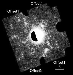
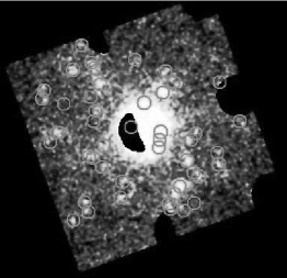
Figure 1.— (left) A Mosaic image of Abell 1689, created with $0.5-10.0$ keV XIS-FI (XIS0 $+$ XIS3) images smoothed with a Gaussian kernel of $\sigma=10^{\prime\prime}$. Background is not subtracted and vignetting is not corrected. CCD regions where ⁵⁵Fe calibration sources are irradiated (Koyama et al. (2007)) are excluded. (right) the same as the left panel, but point-source regions are specified as circles of $1^{\prime}$ radius. See text for details of the point-source detection.

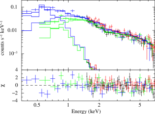
Figure 2.— NXB-subtracted XIS spectra of N4636_GAL and Q1334, fitted with the X-ray background model described in § 3.2. Black and red are 1.5–7.0 keV XIS-FI (averaged over XIS0 and XIS3) and 1.5–7.0 keV XIS-BI spectra of N4636_GAL, respectively. Green and blue are 0.5–7.0 keV XIS-FI and 0.3–7.0 keV XIS-BI spectra of Q1334, respectively.

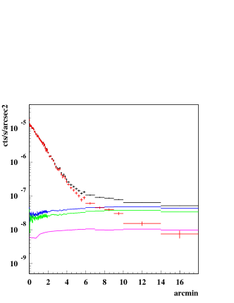
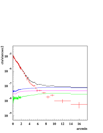
Figure 3.— (left) Surface brightness profiles made of 0.5–2 keV XIS-FI (averaged over XIS0 and XIS3) image, using all the Offset1 through Offset4 observations. Point sources specified in figure 1 (right) are removed, but vignetting is not corrected. Raw (background inclusive) profile (black) is shown with XRB (green), NXB (magenta), and XRB$+$NXB (blue) profiles. A resulting background-subtracted profile (black $-$ blue) is shown in red. The error bars in these profiles are 1$\sigma$. In the error bars in the red profile, 1$\sigma$ uncertainties of the XRB and NXB are added in quadrature to the corresponding statistical 1$\sigma$ errors. (right) the same as the left panel, but for 2–10 keV profiles.

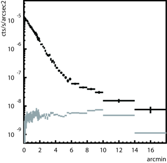
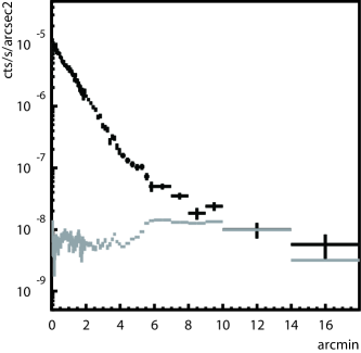
Figure 4.— (left) A simulated 0.5–2 keV profile of residual point source signals (gray), shown with background-subtracted 0.5–2 keV surface brightness profile of XIS-FI averaged over XIS0 and XIS3 (black). In the error bars in this black profile, 1$\sigma$ uncertainties of the XRB and NXB are added in quadrature to the corresponding statistical 1$\sigma$ errors. (right) the same as the left panel, but for 2–10 keV profiles.

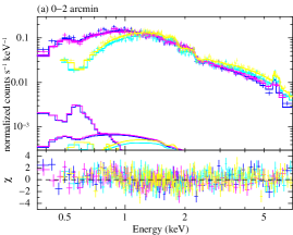
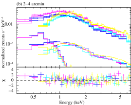
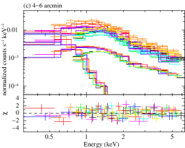
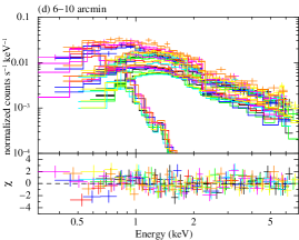
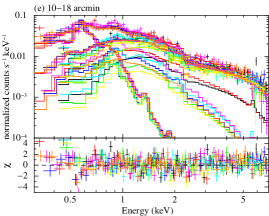
Figure 5.— NXB-subtracted spectra of (a) $0^{\prime}$–$2^{\prime}$, (b) $2^{\prime}$–$4^{\prime}$, (c) $4^{\prime}$–$6^{\prime}$, (d) $6^{\prime}$–$10^{\prime}$, and (e) $10^{\prime}$–$18^{\prime}$ regions, which are extracted from Offset1 XIS-FI (black), Offset1 XIS-BI (red), Offset2 XIS-FI (green), Offset2 XIS-BI (blue), Offset3 XIS-FI (cyan), Offset3 XIS-BI (magenta), Offset4 XIS-FI (yellow), and Offset4 XIS-BI (orange). These spectra are fitted simultaneously with phabs $\times$ apec model, added to the XRB (GFE and CXB) model (§ 3.2). Although blank-sky spectra are also fitted simultaneously with the XRB model, they are not plotted here for clarity. See text for details of the spectral analysis (§ 4.3).

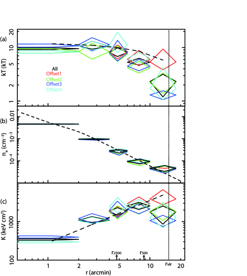
Figure 6.— (a) Projected temperature profiles obtained by spectral analyses of Offset1 (red), Offset2 (green), Offset3 (blue), and Offset4 (cyan) observations. A temperature profile when all spectra of azimuthal regions at the same distance are summed is also shown in black. Dashed line is a temperature profile, $kT=12.3-7.7\;(r/15\farcm 6)$ keV, expected from the scaled temperature profile by Pratt et al. (2007). Dotted line shows the virial radius ($15\farcm 6$). Arrows are the positions of $r_{\rm 500}$ ($8\farcm 7$) and $r_{\rm 2500}$ ($4\farcm 7$). (b) the same as panel (a), but for deprojected electron number density profiles. See text for the detailed method of derivation (§ 4.3). Dashed line shows a model profile by Peng et al. (2009) (Model 3 in table 9). (c) the same as panel (a), but for entropy profiles obtained by calculating $K=kT/n^{2/3}$ from profiles in panel (a) and (b). Dashed line shows $K\propto r^{1.1}$. Normalization of dashed line is arbitrarily scaled.

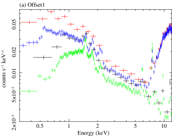
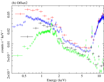
Figure 7.— (a) Raw XIS-FI (black; averaged over XIS0 and XIS3) and XIS-BI (red) spectra of the Offset1 $10\farcm 0$–$18\farcm 0$ region, and corresponding background spectra of XIS-FI (green) and XIS-BI (blue). Each background spectrum was created by adding NXB and XRB spectra. The XRB spectrum was simulated using fakeit command in XSPEC12, incorporating the GFE and CXB models detemined by the spectral fitting described in § 4.3. (b) The same as panel (a), but for the Offset2 $10\farcm 0$–$18\farcm 0$ region.

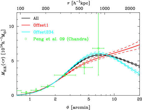
Figure 8.— The hydrostatic equilibrium mass profile. The black, red and light blue colors represent the hydrostatic equilibrium mass for all, Offset1 and Offset234 regions, respectively. The solid and dashed lines indicate the best fit values and the 68% CL uncertainty errors obtained from Monte Carlo simulations, respectively. The green points are the model-independent mass based on the Chandra observation by Peng et al. (2009), which agrees with our results. The unphysical declines in the cumulative masses (all and Offset234) indicate that the ICM of the outskirts is far from hydrostatic equilibrium we assumed.

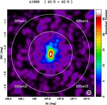
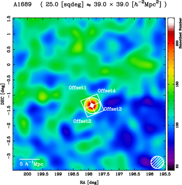
Figure 9.— The two-dimensional density distributions of galaxies around A1689, retrieved from SDSS photometric data. (left) : Distributions of red sequence galaxies of Abell 1689. The box size is $40\farcm 0\times 40\farcm 0$. The annulus is the outskirts region for spectral fitting, where inner and outer circles are $10\farcm 0$ and $18\farcm 0$, respectively. The central distribution is clearly elongated along the north-south direction. We could not find a significant difference between projected distributions in the Offset1 and the other directions. (right) : Distributions of galaxies whose photometric redshifts span in the range of $|z-z_{\rm c}|\leq 0.016$, where $z_{\rm c}$ is the cluster redshift. The boxes represent the FOVs of XIS pointings. The circle is the virial radius determined by lensing analysis. A Gaussian smoothing scale is represented by the hatched circle at bottom right in each plot.

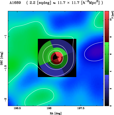
Figure 10.— Gas temperature map of Abell 1689 (shown in the black box), embedded in the SDSS galaxy map which is a magnification of figure 9 (right). Contours of the galaxy map are also overplotted for comparison. The temperatures are the best-fit values determined by the spectral analysis in § 4.3. See figure 6(a) or table 5 for their errors.

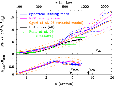
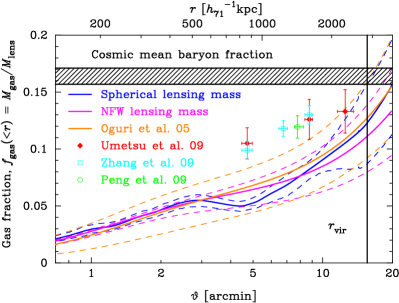
Figure 11.— (left): Comparison of lensing mass, obtained from joint strong and weak lensing analysis, and hydrostatic mass. Blue, magenta and orange colors represent deprojected spherical lensing mass, NFW one, and triaxial halo model (Oguri et al., 2005), respectively. Black line represents the hydrostatic mass in all directions within the radius $r\sim 7\farcm 0$, outside which the hydrostatic equilibrium is not adequate any more (figure 8). The solid and dashed lines are the best fit values and the 68% CL uncertainty errors obtained from Monte Carlo simulations, respectively. Green points are the hydrostatic mass using Chandra data (Peng et al., 2009). The arrows denote the overdensity radii $r_{2500}$ and $r_{500}$ determined by deprojected spherical lensing mass. (right): Cumulative gas mass fraction. Blue, magenta and orange colors represent gas mass fractions using deprojected spherical lensing mass, NFW one, and triaxial halo model (Oguri et al., 2005), respectively. The solid and dashed lines are the same as left panel. Red points are the gas mass fraction based on AMiBA SZE measurement and Subaru lensing analysis for 4 clusters (Umetsu et al., 2009a), at three overdensities $\Delta=2500,500~{}\&~{}200$. Light blue points are the gas mass fraction based on XMM-Newton X-ray and Subaru lensing analysis for 12 clusters of LoCuSS project (Zhang et al., 2010), at three overdensities $\Delta=2500,1000~{}\&~{}500$. Green point denotes the gas fraction using Chandra hydrostatic mass for A1689 (Peng et al., 2009). In this figure, we use $h_{71}=H_{0}/71\;\rm{km\;s^{-1}\;Mpc^{-1}}=1.0$.

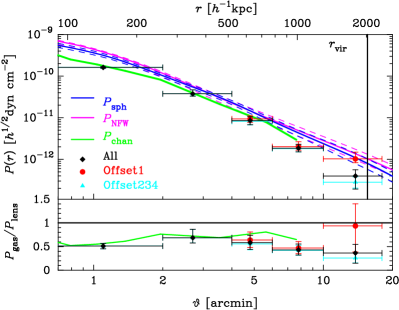
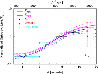
Figure 12.— (left): Comparison of the gas thermal pressure with the total pressure expected from lensing masses with hydrostatic equilibrium assumption. Blue and magenta colors are the pressure calculated from deprojected spherical lensing mass and NFW one, respectively. Solid and dashed lines represent the best and $\pm 1\sigma$ errors, respectively. Black, red and light blue points are observed thermal pressures (68% confidence errors) in the all, Offset1 and Offset234, respectively. Green line in the left panel is the pressure of Chandra data (Peng et al., 2009). (right): The normalized entropy profiles. The colors are the same as those in the left panel. The slope of the entropy in Offset1 is in good agreement with that expected from lensing masses with hydrostatic equilibrium assumption.

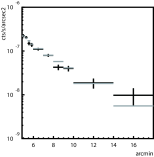
Figure 13.— Simulated 6.2 keV apec (gray) profile is shown, which follows the double-beta profile determined from the 0.5–10 keV XMM-Newton MOS1 image as described in § 2.2. For comparison, background-subtracted 0.5–10 keV surface brightness profile of XIS-FI averaged over XIS0 and XIS3 (black) is also shown. In this black profile, the residual contribution of point sources estimated in § 4.2 is also subtracted. In the error bars of the red profile, 1$\sigma$ uncertainties of the XRB and NXB are added in quadrature to the corresponding statistical 1$\sigma$ errors.

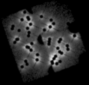
Figure 14.— A simulated 0.5–10 keV XIS-FI (XIS0 $+$ XIS3) mosaic image of point sources, smoothed with a gaussian kernel of $\sigma=10^{\prime\prime}$. $1^{\prime}$ circular regions around these sources are excluded. Simulated exposures of the 4 observations are set 10 times longer than the actual ones.

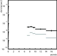
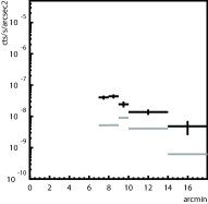
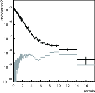
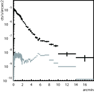
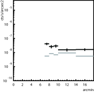
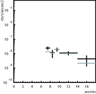
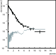
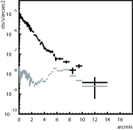
Figure 15.— (top) Simulated 0.5–2 keV profiles of residual point source signals (gray) in Offset1 through Offset4 pointings from left to right, shown with background-subtracted 0.5–2 keV surface brightness profile of XIS-FI averaged over XIS0 and XIS3 (black). In the error bars in this black profile, 1$\sigma$ uncertainties of the XRB and NXB are added in quadrature to the corresponding statistical 1$\sigma$ errors. (bottom) the same as the top panels, but for 2–10 keV profiles.

Table 1 Suzaku Observation log of Abell 1689.

Observation (ID)	Start	End	Exposure
Offset1 (803024010)	2008/July/23 04:42:40	2008/July/24 08:22:23	39.2
Offset2 (803025010)	2008/July/24 08:23:04	2008/July/25 10:09:18	38.2
Offset3 (803026010)	2008/July/25 10:09:59	2008/July/26 11:23:19	39.3
Offset4 (803027010)	2008/July/26 11:24:00	2008/July/27 12:13:14	37.9

Table 2RASS averaged count rates around Abell 1689 and the blank-sky fields.

Band	$0.5^{\circ}$–$1.0^{\circ}$	Q1334	N4636_GAL
1/4 keV	$858.3\pm 36.0$	$816.1\pm 28.0$	$1072.1\pm 42.1$
3/4 keV	$157.6\pm 15.8$	$133.3\pm 12.0$	$238.3\pm 20.1$
1.5 keV	$139.1\pm 14.3$	$132.2\pm 12.0$	$159.2\pm 17.8$

Table 3Results of model fittings to XIS spectra of the blank sky fields.

$\Gamma$(CXB)	$S_{\rm x}$(CXB)	$S_{\rm x}$(GFE)	$\chi^{2}/$dof
1.412 (fix)	$6.3^{+0.2}_{-0.2}\times 10^{-8}$	$3.5^{+1.2}_{-1.2}\times 10^{-8}$	162.4/127

Table 4Significance of the signal outside $10^{\prime}$.

	Fraction	Significance
Offset1 0.5–2 keV	0.21	5.4$\sigma$
Offset2 0.5–2 keV	0.25	2.9$\sigma$
Offset3 0.5–2 keV	0.45	2.0$\sigma$
Offset4 0.5–2 keV	0.09	2.6$\sigma$
Offset1 2–10 keV	0.47	2.1$\sigma$
Offset2 2–10 keV	0.80	0.0$\sigma$
Offset3 2–10 keV	$>1$	0.0$\sigma$
Offset4 2–10 keV	0.64	0.2$\sigma$

Table 5Fitting results of spectral analysis for the five annular regions.

Region	$kT_{1}$	$Z_{1}$	$kT_{2}$	$Z_{2}$	$kT_{3}$	$Z_{3}$	$kT_{4}$	$Z_{4}$	$\chi^{2}$/D.O.F
$0^{\prime}$–$2^{\prime}$	–	–	$8.55^{+1.01}_{-0.70}$	$0.36^{+0.15}_{-0.15}$	$10.76^{+0.88}_{-0.58}$	$0.34^{+0.09}_{-0.09}$	$8.23^{+0.46}_{-0.42}$	$0.26^{+0.06}_{-0.06}$	$752.0/605$
$2^{\prime}$–$4^{\prime}$	–	–	$8.39^{+3.63}_{-2.33}$	$0.12^{+0.98}_{-0.12}$	$11.39^{+3.92}_{-2.75}$	$0.77^{+0.00}_{-0.77}$	$10.53^{+2.60}_{-1.59}$	$0.49^{+0.26}_{-0.25}$	$273.2/204$
$4^{\prime}$–$6^{\prime}$	$8.42^{+2.76}_{-2.35}$	$0.77^{+0.00}_{-0.77}$	$7.51^{+3.40}_{-2.00}$	$3.76^{+0.00}_{-3.76}$	$7.96^{+5.68}_{-2.38}$	$0.92^{+0.00}_{-0.92}$	$11.19^{+8.15}_{-3.11}$	$0.94^{+1.19}_{-0.94}$	$319.0/210$
$6^{\prime}$–$10^{\prime}$	$5.96^{+2.89}_{-1.39}$	$0.71^{+1.11}_{-0.71}$	$4.14^{+1.48}_{-0.80}$	$1.40^{+2.30}_{-1.17}$	$4.49^{+1.58}_{-0.83}$	$1.21^{+1.65}_{-1.02}$	$6.27^{+1.88}_{-1.21}$	$0.89^{+0.99}_{-0.72}$	$394.3/262$
$10^{\prime}$–$18^{\prime}$	$5.37^{+4.02}_{-1.54}$	$0.64^{+1.07}_{-0.64}$	$2.21^{+1.13}_{-0.83}$	$0.49^{+1.94}_{-0.49}$	$1.30^{+0.26}_{-0.24}$	$0.50^{+1.85}_{-0.38}$	$1.71^{+2.56}_{-0.65}$	$3.65^{+0.00}_{-3.65}$	$665.7/458$
Region	$kT_{\rm all}$				$Z_{\rm all}$				$\chi^{2}$/D.O.F
$0^{\prime}$–$2^{\prime}$	$9.53^{+0.39}_{-0.39}$				$0.31^{+0.05}_{-0.05}$				$822.5/611$
$2^{\prime}$–$4^{\prime}$	$10.58^{+2.55}_{-1.24}$				$0.63^{+0.30}_{-0.31}$				$499.2/210$
$4^{\prime}$–$6^{\prime}$	$8.09^{+1.82}_{-1.30}$				$0.65^{+0.66}_{-0.60}$				$429.7/219$
$6^{\prime}$–$10^{\prime}$	$5.31^{+1.00}_{-0.61}$				$0.90^{+0.58}_{-0.48}$				$423.0/271$
$10^{\prime}$–$18^{\prime}$	$2.32^{+0.85}_{-1.13}$				$0.35^{+0.65}_{-0.31}$				$743.6/467$

Table 6Deprojected electron number densities of the five annular regions.

Region	$n_{\rm e,1}$	$n_{\rm e,2}$	$n_{\rm e,3}$	$n_{\rm e,4}$	$n_{\rm e,all}$
$0^{\prime}$–$2^{\prime}$	–	–	$4.53^{+0.06}_{-0.06}\times 10^{-3}$	$4.70^{+0.07}_{-0.07}\times 10^{-3}$	$4.62^{+0.07}_{-0.07}\times 10^{-3}$
$2^{\prime}$–$4^{\prime}$	–	–	$9.23^{+0.24}_{-0.67}\times 10^{-4}$	$1.00^{+0.04}_{-0.04}\times 10^{-3}$	$9.64^{+0.32}_{-0.56}\times 10^{-4}$
$4^{\prime}$–$6^{\prime}$	$3.02^{+0.14}_{-0.27}\times 10^{-4}$	$2.77^{+0.21}_{-0.88}\times 10^{-4}$	$2.57^{+0.44}_{-0.77}\times 10^{-4}$	$3.14^{+0.44}_{-0.36}\times 10^{-4}$	$2.88^{+0.33}_{-0.63}\times 10^{-4}$
$6^{\prime}$–$10^{\prime}$	$9.21^{+1.63}_{-1.66}\times 10^{-5}$	$8.44^{+2.74}_{-2.48}\times 10^{-5}$	$9.86^{+2.55}_{-2.33}\times 10^{-5}$	$1.04^{+0.14}_{-0.22}\times 10^{-4}$	$9.49^{+2.20}_{-2.22}\times 10^{-5}$
$10^{\prime}$–$18^{\prime}$	$5.18^{+0.62}_{-0.59}\times 10^{-5}$	$4.22^{+1.61}_{-1.10}\times 10^{-5}$	$4.27^{+2.01}_{-1.50}\times 10^{-5}$	$4.99^{+1.28}_{-1.82}\times 10^{-5}$	$4.66^{+1.47}_{-1.33}\times 10^{-5}$

Table 7Best-fit parameters for electron density and temperature profiles.

Region	$n_{\rm e,0}$	$\beta$	$r_{\rm c,1}$	$T_{\rm 0}$	$\alpha$	$r_{\rm t}$
All	$(0.98\pm 0.04)\times 10^{-2}$	$1.16\pm 0.02$	$1.43\pm 0.06$	$19.39\pm 0.61$	$1.03\pm 0.07$	$3.88\pm 0.29$
Offset1	$(1.01\pm 0.11)\times 10^{-2}$	$1.13\pm 0.03$	$1.36\pm 0.13$	$15.85\pm 1.30$	$0.60\pm 0.10$	$2.42\pm 0.53$
Offset234	$(0.97\pm 0.04)\times 10^{-2}$	$1.17\pm 0.02$	$1.44\pm 0.06$	$21.10\pm 1.32$	$1.32\pm 0.19$	$4.72\pm 0.69$

Table 8Lensing Mass Parameters

Model	$M_{\rm vir}$	$C_{\rm vir}$
	$(10^{15}h^{-1}M_{\sun})$
NFW	$1.47^{+0.59}_{-0.33}$	$12.7\pm 2.9$
Spherical	$1.30_{-0.39}^{+0.38}$	-
NFW-equivalent triaxial model	$1.26^{+0.28}_{-0.49}$	$16.9^{+2.2}_{-12.9}$

Table 9Point sources identified in XIS FOVs of Offset1 through Offset4 observations.

#	$\alpha$	$\delta$	Flux
1∗	198.03427	-1.1213164	3.09405e-14
2∗	198.05514	-1.5692276	2.44946e-14
3∗	198.02596	-1.5233972	2.57838e-14
4	197.82543	-1.2416705	1.10009e-13
5	197.78077	-1.4828847	7.7066e-14
6	197.79435	-1.5023029	8.81786e-14
7	197.98643	-1.2203908	4.71844e-14
8	197.76312	-1.4169539	9.32276e-14
9	197.81012	-1.5273204	1.33557e-13
10	197.87293	-1.2675864	2.20443e-14
11	197.98223	-1.4325242	3.78360e-14
12	197.93268	-1.5117554	5.33448e-14
13	197.73176	-1.4571297	4.04592e-14
14	197.74045	-1.3452808	2.70100e-14
15	198.01117	-1.2532794	1.20219e-14
16	198.00135	-1.1785807	3.28471e-14
17	198.00404	-1.4098294	1.87843e-14
18	197.92967	-1.4700792	3.34677e-14
19	197.74718	-1.4467673	3.20633e-14
20	197.68538	-1.3966633	2.40137e-14
21	197.75135	-1.3633463	2.00829e-14
22	198.01480	-1.4067640	2.44474e-14
23	197.97641	-1.3787678	2.09356e-14
24	197.77143	-1.5433937	2.80542e-14
25	197.80647	-1.5398204	4.97257e-14
26	197.89749	-1.1571900	2.98196e-14
27	198.09163	-1.3433972	7.37440e-14
28	198.00850	-1.1652682	5.30538e-14
29	198.09833	-1.3442155	3.14757e-14
30	197.82983	-1.3427566	1.38139e-14
31	197.83316	-1.3627567	3.39411e-14
32	197.83539	-1.3827567	1.35029e-14
33∗	197.90652	-1.3305344	1.15971e-13
34∗	198.11556	-1.3692246	1.31497e-14
35∗	198.13638	-1.2567236	6.44595e-15
36∗	198.13013	-1.2358911	7.99298e-15
37∗	198.01554	-1.5483976	7.99298e-15
38∗	197.74461	-1.5254812	4.89892e-15
39∗	198.08012	-1.2713117	7.21947e-15
40	197.99885	-1.2879834	5.73211e-15
41∗	198.00302	-1.3150664	6.44595e-15
42	197.62584	-1.3150565	1.38741e-13
43	197.79672	-1.2150684	2.26699e-14
44	197.81756	-1.1859025	2.09468e-14
45∗	197.65711	-1.2358936	3.09405e-15
46∗	197.67795	-1.2150621	2.06270e-15
47∗	198.19683	-1.3671319	1.03135e-14
48	198.05636	-1.1827708	2.38688e-14
49	197.67990	-1.4259208	4.19095e-14

References

- Abazajian et al. (2009) Abazajian, K. N., Adelman-McCarthy, J. K., Agüeros, M. A., Allam, S. S., Allende P. C., An, D., Anderson, K. S. J., Anderson, S. F., et al. 2009, ApJS, 182, 543
- Afshordi et al. (2007) Afshordi, N., Lin, Y.-T., Nagai, D., & Sanderson, A. J. R. 2007, MNRAS, 378, 293
- Akahori & Yoshikawa (2009) Akahori, T. & Yoshikawa, K. 2009, PASJ, submitted. Preprint: arXiv0909.5025
- Anders & Grevesse (1989) Anders, E., & Grevesse, N. 1989, GeCoA, 53, 197
- Atrio-Barandela et al. (2008) Atrio-Barandela, F., Kashlinsky, A., Kocevski, D. & Ebeling, H. 2008, ApJ, 675, L57
- Bautz et al. (2009) Bautz, M. W., Miller, E. D., Sanders, J. S., Arnaud, K. A., Mushotzky, R. F., Porter, F. S., Hayashida, K., Henry, J. P., et al. 2009, PASJ, 61, 1117
- Bode et al. (2009) Bode, P., Ostriker, J. P. & Vikhlinin, A. 2009, ApJ, 700, 989
- Borgani et al. (2005) Borgani, S., Finoguenov, A., Kay, S. T., Ponman, T. J., Springel, V., Tozzi, P., & Voit, G. M. 2005, MNRAS, 361, 233
- Broadhurst et al. (2005a) Broadhurst, T., Benítez, N., Coe, D., Sharon, K., Zekser, K., White, R., Ford, H., Bouwens, R., et al. 2005, ApJ, 621, 53
- Broadhurst et al. (2005b) Broadhurst, T., Takada, M., Umetsu, K., Kong, X., Arimoto, N., Chiba, M., & Futamase, T. 2005, ApJ, 619, L143
- Broadhurst & Barkana (2008) Broadhurst, T. & Barkana, R. 2008, MNRAS, 390, 1647
- Bullock et al. (2001) Bullock, J. S., Kolatt, T. S., Sigad, Y., Somerville, R. S., Kravtsov, A. V., Klypin, A. A., Primack, J. R. & Dekel, A. 2001, MNRAS, 321, 559
- Cavaliere & Fusco-Femiano (1976) Cavaliere, A., & Fusco-Femiano, R. 1976, A&A, 49, 137
- Cavaliere et al. (2009) Cavaliere, A., Lapi, A., & Fusco-Femiano, R. 2009, ApJ, 698, 580
- Corless et al. (2009) Corless, V. L., King, L. J., & Clowe, D. 2009, MNRAS, 393, 1235
- Croston et al. (2008) Croston, J. H., Pratt, G. W., Böhringer, H., Arnaud, M., Pointecouteau, E., Ponman, T. J., Sanderson, A. J. R., Temple, R. F., et. al 2008, A&A, 487, 431
- Dickey & Lockman (1990) Dickey, J. M., & Lockman, F. J. 1990, ARA&A, 28, 215
- Dolag et al. (2005) Dolag, K., Vazza, F., Brunetti, G. & Tormen, G. 2005, MNRAS, 364, 753
- Ettori & Fabian (1998) Ettori, S. & Fabian, A. C. 1998, MNRAS, 293, L33
- Faltenbacher et al. (2007) Faltenbacher, A., Hoffman, Y., Gottlöber, S., & Yepes, G. 2007, MNRAS, 376, 1327
- Fang et al. (2009) Fang, T., Humphrey, P., & Buote, D. 2009, ApJ, 691, 1648
- Fox & Loeb (1997) Fox, D. C., & Loeb, A. 1997, 491, 459
- Fujita et al. (2008) Fujita, Y., Tawa, N., Hayashida, K., Takizawa, M., Matsumoto, H., Okabe, N., & Reiprich, T. H. 2008, PASJ, 60, 343
- Gavazzi (2005) Gavazzi, R. 2005,A&A, 443, 793
- George et al. (2009) George, M. R., Fabian, A. C., Sanders, J. S., Young, A. J., & Russell, H. R. 2009, MNRAS, 395, 657
- Hamana et al. (2003) Hamana, T., Miyazaki, S., Shimasaku, K., Furusawa, H., Doi, M., Hamabe, M., Imi, K., Kimura, M., et al. 2003, ApJ, 597, 98
- Hamana et al. (2009) Hamana, T., Miyazaki, S., Kashikawa, N., Ellis, R. S., Massey, R. J., Refregier, A., Taylor, J. E. 2009, PASJ, 61, 833
- Henley & Shelton (2008) Henley, D. B., & Shelton, R. L. 2008, ApJ, 676, 335
- Ishisaki et al. (2007) Ishisaki, Y., Maeda, Y., Fujimoto, R., Ozaki, M., Ebisawa, K., Takahashi, T., Ueda, Y., Ogasaka, Y., et. al 2007, PASJ, 59, 113
- Jeltema et al. (2008) Jeltema, T. E., Hallman, E. J., Burns, J. O., & Motl, P. M. 2008, ApJ, 681, 167
- King (1962) King, I. R. 1962, AJ, 67, 471
- Komatsu & Seljak (2001) Komatsu, E. & Seljak, U. 2001, MNRAS, 327, 1353
- Komatsu et al. (2009) Komatsu, E., Dunkley, J., Nolta, M. R., Bennett, C. L., Gold, B., Hinshaw, G., Jarosik, N., Larson, D., et al. 2009, ApJS, 180, 330
- Koyama et al. (2007) Koyama, K., Tsunemi, H.,; Dotani, T., Bautz, M. W., Hayashida, K., Tsuru, T. G., Matsumoto, H., Ogawara, Y., et al. 2007, PASJ, 59, 23
- Kushino et al. (2002) Kushino, A., Ishisaki, Y., Morita, U., Yamasaki, N. Y., Ishida, M., Ohashi, T., & Ueda, Y. 2002, PASJ, 54, 327
- Lau, Kravtsov, & Nagai (2009) Lau, E. T., Kravtsov, A. V., & Nagai, D. 2009, ApJ, 705, 1129
- Lapi & Cavaliere (2009) Lapi, A. & Cavaliere, A. 2009, ApJ, 692, 174
- Lemze et al. (2009) Lemze, D., Broadhurst, T., Rephaeli, Y., Barkana, R., & Umetsu, K. 2009, ApJ, 701, 1336
- Limousin et al. (2007) Limousin, M. 2007, ApJ, 668, 643
- Mitsuda et al. (2007) Mitsuda, K., Bautz, M., Inoue, H., Kelley, R. L., Koyama, K., Kunieda, H., Makishima, K. Ogawara, Y., et al. 2007, 59, S1
- Miyazaki et al. (2002) Miyazaki, S., Komiyama, Y., Sekiguchi, M., Okamura, S., Doi, M., Furusawa, H., Hamabe, M., Imi, K., et al. 2002, PASJ, 54, 833
- Molnar et al. (2009) Molnar, S. M., Hearn, N., Haiman, Z., Bryan, G., Evrard, A. E., & Lake, G. 2009, ApJ, 696, 1640
- Molnar et al. (2010) Molnar, S. et al. 2010, submitted to ApJL
- Nagai & Kravtsov (2003) Nagai, D. & Kravtsov, A. V. 2003, ApJ, 587, 514
- Nagai, Vikhlinin, & Kravtsov (2007) Nagai, D., Vikhlinin, A., & Kravtsov, A. V. 2007, ApJ, 655, 98
- Nakamura & Suto (1997) Nakamura, T. T., & Suto, Y. 1997, Prog.Theor.Phys., 97, 49
- Nakazawa et al. (2009) Nakazawa, K., Sarazin, C. L., Kawaharada, M., Kitaguchi, T., Okuyama, S., Makishima, K., Kawano, N., Fukazawa, Y., et al. 2009, PASJ, 61, 339
- Navarro, Frenk, & White (1996) Navarro, J. F., Frenk, C. S., & White, S. D. M. 1996, ApJ, 462, 563
- Navarro, Frenk, & White (1997) Navarro, J. F., Frenk, C. S., & White, S. D. M. 1997, ApJ, 490, 493
- Neto et al. (2007) Neto, A. F., Gao, L., Bett, P., Cole, S., Navarro, J. F., Frenk, C. S., White, S. D. M., Springel, V., et al. 2007, MNRAS, 381, 1450
- Oguri et al. (2005) Oguri, M., Takada, M., Umetsu, K., & Broadhurst, T. 2005, ApJ, 632, 841
- Oguri et al. (2009) Oguri, M., Hennawi, J. F., Gladders, M. D., Dahle, H., Natarajan, P., Dalal, N., Koester, B. P., Sharon, K. & Bayliss, M. 2009, ApJ, 699, 1038
- Okabe & Umetsu (2008) Okabe, N., & Umetsu, K. 2008, PASJ, 60, 345
- Okabe et al. (2009) Okabe, N., Takada, M., Umetsu, K., Futamase, T., & Smith, G. P. 2009, PASJ submitted. Preprint: arXiv:0903.1103
- Okabe et al. (2010) Okabe, N., Zhang, Y.,-Y., Finoguenov, A., Takada, M., Umetsu, K., Smith, G. P., & Futamase, T. 2010, ApJ submitted.
- Ostriker et al. (2005) Ostriker, J. P., Bode, P., & Babul, A. 2005, ApJ, 634, 964
- Piffaretti et al. (2003) Piffaretti, R., Jetzer, P., & Schindler, S. 2003, A&A, 398, 41
- Piffaretti & Valdarnini (2008) Piffaretti, R., & Valdarnini, R. 2008, A&A, 491, 71
- Peng et al. (2009) Peng, E.-H., Andersson, K., Bautz, M. W., & Garmire, G. P. 2009, ApJ, 701, 1283
- Ponman et al. (2003) Ponman, T. J., Sanderson, A. J. R., & Finoguenov, A. 2003, MNRAS, 343, 331
- Pratt et al. (2006) Pratt, G. W., Arnaud, M., & Pointecouteau, E. 2006, A&A, 446, 429
- Pratt et al. (2007) Pratt, G. W., Böhringer, H., Croston, J. H., Arnaud, M., Borgani, S., Finoguenov, A., & Temple, R. F. 2007, A&A, 461, 71
- Reiprich et al. (2009) Reiprich, T. H., Hudson, D. S., Zhang, Y. -Y., Sato, K., Ishisaki, Y., Hoshino, A., Ohashi, T., Ota, N., et al. 2009, A&A, 501, 899
- Ryu et al. (2003) Ryu, D., Kang, H., Hallman, E., & Jones, T. W. 2003, ApJ, 593, 599
- Serlemitsos et al. (2007) Serlemitsos, P. J., Soong, Y., Chan. K., Okajima, T., Lehan, J. P., Maeda, Y., Itoh, K., Mori, H., et al. 2007, PASJ, 59, 9
- Smith et al. (2001) Smith, R. K., Brickhouse, N. S., Liedahl, D. A., & Raymond, J. C. 2001, ApJ, 556, L91
- Snowden et al. (2008) Snowden, S. L., Mushotzky, R. F., Kuntz, K. D., & Davis, D. S. 2008, A&A, 478, 615
- Spitzer (1962) Spitzer, L. Jr. 1962, Physics of Fully Ionized Gases (New York: Wiley)
- Struble & Rood (1999) Struble, M. F., & Rood, H. J. 1999, ApJS, 125, 35
- Sunyaev & Zeldovich (1972) Sunyaev, R. A., & Zeldovich, Y. B. 1972, Comments Astrophys. Space Phys., 4, 173
- Takahashi et al. (2008) Takahashi, T., Kelley, R., Mitsuda, K., Kunieda, H., Petre, R., White, N., Dotani, T., Fujimoto, R., et al. 2008, Proc. SPIE, 7011, 70110O
- Takizawa (1998) Takizawa, M. 1998, ApJ, 509, 579
- Takizawa (1999) Takizawa, M. 1999, ApJ, 520, 514
- Tawa et al. (2008) Tawa, N., Hayashida, K., Nagai, M., Nakamoto, H., Tsunemi, H., Yamaguchi, H., Ishisaki, Y., Miller, E. D., et al. 2008, PASJ, 60, 11
- Taylor & Navarro (2001) Taylor, J. E., & Navarro, J. F. 2001, ApJ, 563, 483
- Tozzi & Norman (2001) Tozzi P., & Norman, C. 2001, ApJ, 546, 63
- Umetsu & Broadhurst (2008) Umetsu, K., & Broadhurst T. 2008, ApJ, 684, 177
- Umetsu et al. (2009a) Umetsu, K., Birkinshaw, M., Liu, G., Wu, J. P., Medezinski, E., Broadhurst, T., Lemze, D., Zitrin, A., et al. 2009, ApJ, 694, 1643
- Umetsu et al. (2009b) Umetsu, K., Medezinski, E., Broadhurst, T., Zitrin, A., Okabe, N., Hsieh, B. C., & Molnar, S. M. 2009, ApJ submitted. Preprint: arXiv0908.0069
- Vazza et al. (2009) Vazza, F., Brunetti, G., Kritsuk, A., Wagner, R., Gheller, C., & Norman, M. 2009, A&A, 504, 33
- Vikhlinin et al. (1999) Vikhlinin, A., Forman, W., & Jones, C. 1999, ApJ, 525, 47
- Vikhlinin et al. (2006) Vikhlinin, A., Kravtsov, A., Forman, W., Jones, C., Markevitch, M., Murray, S. S., & Van Speybroeck, L. 2006, ApJ, 640, 691
- Vikhlinin et al. (2009) Vikhlinin, A., Burenin, R. A., Ebeling, H., Forman, W. R., Hornstrup, A., Jones, C., Kravtsov, A. V., Murray, S. S., et al. 2009, ApJ, 692, 1033
- Voit et al. (2002) Voit, G. M., Bryan, G. L., Balogh, M. L., & Bower, R. G. 2002, ApJ, 601
- Watson (2009) Watson, M. G., Schröder, A. C., Fyfe, D., Page, C. G., Lamer, G., Mateos, S., Pye, J., Sakano, M., et al. 2009, A&A, 493, 339
- Zhang et al. (2006) Zhang, Y.-Y., Böhringer, H., Finoguenov, A., Ikebe, Y., Matsushita, K., Schuecker, P., Guzzo, L., & Collins, C. A. 2006, A&A, 456, 55.
- Zhang et al. (2007) Zhang, Y.-Y., Finoguenov, A., Böhringer, H., Kneib, J.-P., Smith, G. P., Czoske, O. & Soucail, G. 2007, A&A, 467, 437
- Zhang et al. (2008) Zhang, Y.-Y., Finoguenov, A., Böhringer, H., Kneib, J.-P., Smith, G. P., Kneissl, R., Okabe, N., & Dahle, H. 2008, A&A, 482, 451
- Zhang et al. (2010) Zhang., Y-., Y., Okabe, N., Finoguenov, A., Graham, P. S., Piffaretti., R., Valdarnini, R., Babul, A., Evrard, A. E., et al. 2010 ApJ submitted. Preprint: arXiv:1001.0780