Photometric determination of the mass accretion rates of pre-main sequence stars. I.
Method and application to the SN 1987A field

Abstract

We have developed and successfully tested a new self-consistent method to reliably identify pre-main sequence (PMS) objects actively undergoing mass accretion in a resolved stellar population, regardless of their age. The method does not require spectroscopy and combines broad-band $V$ and $I$ photometry with narrow-band $H\alpha$ imaging to: (1) identify all stars with excess H$\alpha$ emission; (2) convert the excess H$\alpha$ magnitude into H$\alpha$ luminosity $L(H\alpha)$; (3) estimate the H$\alpha$ emission equivalent width; (4) derive the accretion luminosity $L_{\rm acc}$ from $L(H\alpha)$; and finally (5) obtain the mass accretion rate $\dot{M}_{\rm acc}$ from $L_{\rm acc}$ and the stellar parameters (mass and radius). By selecting stars with an accuracy of 15 % or better in the H$\alpha$ photometry, the statistical uncertainty on the derived $\dot{M}_{\rm acc}$ is typically $\lesssim 17\,\%$ and is dictated by the precision of the H$\alpha$ photometry. Systematic uncertainties, of up to a factor of 3 on the value of $\dot{M}_{\rm acc}$, are caused by our incomplete understanding of the physics of the accretion process and affect all determinations of the mass accretion rate, including those based on a spectroscopic H$\alpha$ line analysis.

As an application of our method, we study the accretion process in a field of $9.16$ arcmin${}^{2}$ around SN 1987A, using existing Hubble Space Telescope photometry. We identify as bona-fide PMS stars a total of 133 objects with a H$\alpha$ excess above the $4\,\sigma$ level and a median age of $13.5$ Myr. Their median mass accretion rate of $2.6\times 10^{-8}$ M${{}_{\odot}}$  yr${}^{-1}$ is in excellent agreement with previous determinations based on the $U$-band excess of the stars in the same field, as well as with the value measured for G-type PMS stars in the Milky Way. The accretion luminosity of these PMS objects shows a strong dependence on their distance from a group of hot massive stars in the field and suggests that the ultraviolet radiation of the latter is rapidly eroding the circumstellar discs around PMS stars.

1. Introduction

In the current star formation paradigm, low-mass stars grow in mass over time through accretion of matter from a circumstellar disc (e.g. Lynden-Bell & Pringle 1974; Appenzeller & Mundt 1989; Bertout 1989). This accretion process is believed to occur via the magnetic field lines that connect the star to its disc and that act as funnels for the gas (e.g. Königl 1991; Shu et al. 1994). The strong excess emission observed in most of these pre-main sequence (PMS) stars is believed to originate through gravitational energy, released by infalling matter, that ionises and excites the gas. Thus, the excess luminosity of these objects (the classical T Tauri stars) can be used to measure the mass accretion rate.

A reliable measurement of the rate of mass accretion onto PMS stars is of paramount importance for understanding the evolution of both the stars and their discs (see e.g. review by Calvet et al. 2000). Of particular interest is determining how the mass accretion rate changes with time as a star approaches its main sequence, whether it depends on the final mass of the forming star and whether it is affected by the chemical composition and density of its parent molecular cloud or by the proximity of hot, massive stars.

Ground-based spectroscopic studies of nearby young star-forming regions (e.g. in Taurus, Auriga, Ophiuchus, Orion) show that the mass accretion rate appears to decrease steadily with time, from $\sim 10^{-8}$ M${{}_{\odot}}$  yr${}^{-1}$ at ages of $\sim 1$ Myr to $<10^{-9}$ M${{}_{\odot}}$  yr${}^{-1}$ at $\sim 10$ Myr (Muzerolle et al. 2000; Sicilia-Aguilar et al. 2005; 2006). While at face value this is in line with the expected evolution of viscous discs (Hartmann et al. 1998), the scatter on the data is very large, exceeding 2 dex at any given age. This is at least in part explained by the recent finding that the mass accretion rate seems also to depend quite steeply on the mass of the forming star. Muzerolle et al. (2003; 2005), Natta et al. (2004; 2006), White & Hillenbrand (2004) and Sicilia-Aguilar et al. (2006) consistently report that the accretion rate $\dot{M}_{\rm acc}$ decreases with the stellar mass $M$ as $\dot{M}_{\rm acc}\propto M^{2}$, albeit with large uncertainties on the actual value of the power-law index. On the other hand, Clarke & Pringle (2006) warn that such a steep decline might be spurious and strongly driven by detection/selection thresholds.

While observational uncertainties and potential systematic errors may well contribute to the present uncertainty, the true limitation in this field of research currently comes from the paucity of available measurements. Indeed, all the results so far obtained are based on the mass accretion rates of a small number of stars (just over one hundred), all located in nearby Galactic star forming regions, covering a very limited range of ages and no appreciable range of metallicity (all clouds mentioned above having essentially solar metallicity; e.g. Padgett 1996).

The origin of this limitation is to be found in the technique used to measure PMS mass accretion rates. Regardless as to whether the latter are derived from the analysis of veiling in the photosperic absorption lines (usually at ultraviolet and optical wavelengths) or through a detailed study of the profile and intensity of emission lines (usually H$\alpha$, Pa$\beta$ or Br$\gamma$), these thechniques typically require medium to high resolution spectroscopy for each individual object. Even with modern multi-object spectrographs at the largest ground-based telescopes, this approach is not very efficient and cannot reach beyond nearby star forming regions or the Orion cluster, as crowding and sensitivity issues rule out but the brightest objects in more distant regions like the centre of the Milky Way or the Magellanic Clouds. While in principle the PMS mass accretion rate can be estimated from the $U$-band excess if the spectral type is known (see e.g. Gullbring et al. 1998; Romaniello et al. 2004), this method is potentially subject to large uncertainties in the extinction and in the determination of the correct spectral type and effective temperature when spectroscopy is not available.

In order to overcome these limitations and significantly extend the sample of stars with a measured mass accretion rate, we have developed and successfully tested a new method to reliably measure $\dot{M}_{\rm acc}$ that does not require spectroscopy. The method, described in the following sections, combines broad-band $V$ and $I$ photometry with narrow-band $H\alpha$ imaging and allows us to identify all stars with excess H$\alpha$ emission and to derive from it the accretion luminosity $L_{acc}$ and hence $\dot{M}_{\rm acc}$ for hundreds of objects simultaneously.

The paper is organised as follows: in Section 2 we address the identification of PMS stars via their colour excess and in Section 3 we show how to reliably convert the measured excess into H$\alpha$ luminosity and equivalent width. Section 4 shows how the accretion luminosity and mass accretion rate can be obtained from the H$\alpha$ luminosity and Section 5 presents an application of the method to the field of SN 1987A, in the Large Magellanic Cloud (LMC). A thorough discussion of all systematic uncertainties involved in the method is provided in Section 6, while a general discussion and conclusions follow in Section 7. The Appendix provides additional figures and tabular material.

2. Identification of PMS stars through their colour excess

One of the characteristic signatures of the accretion process on to PMS stars is the presence of excess emission in H$\alpha$ (see Calvet et al. 2000). Although surveys to search for stars with H$\alpha$ excess emission over large sky areas have been traditionally carried out via slitless spectroscopy (e.g. Herbig 1957; Kohoutek & Wehmeyer 1999), extensive studies in which narrow-band H$\alpha$ imaging is combined with broad-band photometry also exist (e.g. Parker et al. 2005; Drew et al. 2005).

Recently, Romaniello et al. (1998), Panagia et al. (2000) and Romaniello et al. (2006) used HST/WFPC2 photometry in H$\alpha$ (F656N) and the R band (F675W) to provide the first direct detection of extra-galactic PMS stars with strong H$\alpha$ emission in the LMC. Their approach is based on the widely adopted use of the R band magnitude as an indicator of the level of the photospheric continuum near the H$\alpha$ line. Therefore, stars with strong H$\alpha$ emission will have a large $R-H\alpha$ colour. From the analysis of the specific F656N and F675W filter response curves of the WFPC2 instrument, Panagia et al. (2000) conclude that an equivalent width ($W_{\rm eq}$) of the H$\alpha$ emission line in excess of 8 Å   will result in a colour excess $R-H\alpha\gtrsim 0.3$.

This way of identifying PMS stars is more accurate and reliable than the simple classification based on the position of the objects in the Hertzsprung–Russell diagram, i.e. stars placed well above the main sequence (e.g. Gilmozzi et al. 1994; Hunter et al. 1995; Nota et al. 2006; Gouliermis et al. 2007). The reason is twofold: (i) contamination by older field stars and the effects of differential extinction may lead to an overestimate of the actual number of candidate young, low-mass PMS stars, i.e. those “above” the MS; (ii) older PMS stars, already close to their MS, cannot be properly identified with this method, thereby resulting in an underestimate of the number of stars that are still forming. When PMS stars are identified by means of their $R-H\alpha$ colour excess, both problems disappear.

Similarly, this approach is more practical, efficient and economical than slitless spectroscopy for studying PMS stars in dense star forming regions in the Milky Way and nearby galaxies, which are today accessible thanks to high-resolution observations, in particular those made with the HST.

We will show in Section 3 that the level of the photospheric continuum near H$\alpha$ can be directly derived from the observed $V$ and $I$ magnitudes. This means that PMS stars with an H$\alpha$ excess can be identified without actually measuring the canonical $R-H\alpha$ index. On the other hand, since $R-H\alpha$ has traditionally been used in PMS stars studies, we first show here how one can derive analytically the $R$ magnitude of an object from the measured $V$ and I magnitudes. In this way, we intend to make it possible for those who do not dispose of R-band photometry for their fields to derive it in an accurate way by using measurements in the neighbouring V and I bands. The latter are more commonly used than the R band in photometric studies of resolved stellar populations and are particularly popular among HST observers.

2.1. Deriving $R$ from $V$ and $I$

The absence of remarkable spectral features between 5 000 Å  and 9 000 Å  in the stellar continuum of dwarfs and giants with effective temperatures in the range 4 000 K $\lesssim T_{\rm eff}\lesssim$ 10 000 K implies that their $V-R$ and $V-I$ colours depend primarily on the effective temperature of the stars and less on their metallicity. In effect, $V-I$ remains a useful colour index for temperature determinations (von Braun et al. 1998; Bessell, Castelli & Plez 1998).

The colour–colour sequences in the $UBVRIJKLMN$ passbands published by Johnson (1966) revealed a very tight correlation between the mean $V-R$ and $V-I$ colours of local dwarfs and giants (see Figure 1). The correlation is remarkably linear in the range $0<V-I<2$ (i.e. 4 000 K $\lesssim T_{\rm eff}\lesssim$ 10 000 K), where $(V-R)=0.58\times(V-I)$ (dashed line in Figure 1), and it remains linear for $2<V-I<4$ (i.e. 3 000 K $\lesssim T_{\rm eff}\lesssim$ 4 000 K), albeit with a shallower slope ($0.45$; dot-dashed line). It is, therefore, possible and meaningful to attempt to derive the value of the $R$ magnitude from the knowledge of $V$ and $I$, particularly because no extrapolation beyond the available wavelength range is involved. The simple inversion of the relationship above gives $R=0.42\,V+0.58\,I$ for the system of Johnson.

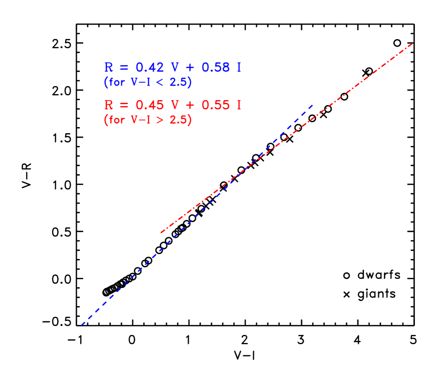
Figure 1.— The tight correlation between $V-R$ and $V-I$ from the colour–colour sequences of Johnson (1966). Circles indicate dwarfs and crosses giants.

Interestingly, this relationship is very similar to the one that we would obtain if we assumed that the proportion with which the $V$ and $I$ magnitudes contribute to the $R$ magnitude is simply dictated by the ratio of the effective wavelengths of the filters. The effective wavelengths of the V, R and I bands in Johnson’s system are, respectively, $\lambda_{e}^{V}=5500$ Å , $\lambda_{\rm e}R=7000$ Å  and $\lambda_{\rm e}^{\rm V}=9000$ Å , which imply that the V band should contribute for $(7000-5500)/(9000-5500)\simeq 0.43$ and the I band for $(9000-7000)/(9000-5500)\simeq 0.57$ to the R-band magnitude. These values are remarkably close to those observed.

The apparent disarming simplicity of this conclusion, however, should not lead one to think that this is the case for any photometric system. In particular, for spectral bands much wider than Johnson’s, such as some of the HST/WFPC2 and HST/ACS filters, the matter becomes more complicated because the true effective wavelength can depend significantly on the spectral properties of the source (i.e. its temperature). In these cases, the relationship should be derived via direct observations in the specific bands or through synthetic photometry, when the properties of the photometric system are well caracterised.

Due to the large number of inter-related observing modes offered by the scientific instruments on board the HST, synthetic photometry has long been established as the most practical and efficient approach to their calibration (see Koornneef et al. 1986; Horne 1988; Sirianni et al. 2005). For this reason, reference tables exist that accurately describe the main optical components of the telescope and instruments as well as the response and quantum efficiency of the detectors as a function of wavelength. Therefore, thanks also to the availability of standardised software packages (e.g. Synphot; see Laidler et al. 2008), it is relatively easy to derive synthetic magnitudes from observed or theoretical stellar spectra for various HST instrumental configurations.

We have used both observed and theoretical stellar spectra, taken respectively from the Bruzual-Persson-Gunn-Stryker (BPGS) Spectrophotometry Atlas (see Gunn & Stryker 1983) and from the stellar atmosphere models of Bessell et al. (1998), to compute colour relationships between $R$-like magnitudes and $V-I$-like colours for various HST instruments and ground photometric systems. Details on how the colour transformations were derived and a table of coefficients (Table LABEL:tab3) can be found in the Appendix, while a brief comparison with HST data is given in the following section.

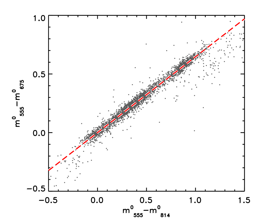
Figure 2.— Colour–colour diagram of all stars in the SN 1987A field with combined mean photometric error $\delta_{3}\leq 0.05$ mag. The dashed line shows the colour relationship derived for the bands in question (F555W, F675W and F814W) from the models of Bessell et al. (1998) and is in excellent agreement with the observations.

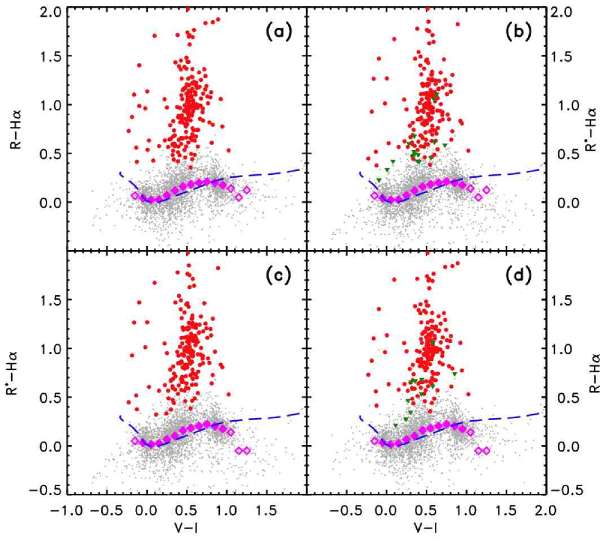
Figure 3.— Comparison between the measured and derived $R-H\alpha$ colour excess. While $R$ denotes the magnitude actually measured in the F675W band, $R^{*}$ indicates the magnitude derived from $V$ (F555W) and $I$ (F814W) by using the relationship of Table LABEL:tab3. Diamonds represent the measured average $R-H\alpha$ colour of the population while the dashed lines is the colour predicted my theoretical models. Thick dots corresponds to stars with $R-H\alpha$ excess larger than $4\,\sigma$. See text for an explanation of the remaining symbols.

2.2. Comparison with the data

To verify the validity of the predicted colour relationships, we have used WFPC2 photometry of a field around SN 1987A studied by Romaniello (1998), Panagia et al. (2000) and Romaniello et al. (2002). The observations cover a field of $9.16$ arcmin${}^{2}$ and were collected over three epochs, namely 1994 September, 1996 February and 1997 July. The advantage of this catalogue is that the magnitude of each star in it is individually corrected for the effects of interstellar extinction by using the information provided simultaneously by all broad-band filters (see Romaniello et al. 2002 for more details). While it would be possible to include the effects of reddening in the calculations of the colour relationships of Table LABEL:tab3, it is more appropriate in this case to correct the observed magnitudes, since considerable differential extinction is likely to be present in this field (see Panagia et al. 2000; De Marchi & Panagia, in preparation).

From the catalogue of Romaniello et al. (2002), we have selected all those stars whose mean error $\delta_{3}$ in the three bands F555W, F675W and F814W does not exceed $0.05$ mag, where

$$\delta_{3}=\sqrt{\frac{\delta^{2}_{555}+\delta^{2}_{675}+\delta^{2}_{814}}{3}}$$ (1)

and $\delta_{555}$, $\delta_{675}$ and $\delta_{814}$ are the photometric uncertainties in each individual band after correction for interstellar extinction. A total of $9\,635$ stars satisfy the condition set by Equation 1, out of $21\,955$ objects in the complete catalogue.

The colour–colour diagram for the stars selected in this way is shown in Figure 2. The dashed line in that figure corresponds to the colour relationship derived for the bands in question from the models of Bessell et al. (1998; see the Appendix) and is practically indistinguishable from the best linear regression fit to the data, which has a slope of $0.645\pm 0.003$. Although these models were selected to match the metallicity of the LMC, having used the relationship derived with the BPGS atlas or that for $[M/H]=-1$ would have still resulted in a very good fit, within the observational uncertainties. This result confirms that, at least over the range explored here, metallicity does not play a dominant role in the colour relationships.

We provide a further proof of the reliability and accuracy of the interpolated R-band magnitudes in Figure 3, where we compare the identification of PMS stars based on the measured and interpolated $R-H\alpha$ colour. To distinguish the observed from interpolated R-band magnitude, we indicate the latter with $R^{*}$, as explained below. In this case, from the photometry of Romaniello et al. (2002) already corrected for reddening, we have further restricted the selection to objects with $\delta_{3}\leq 0.02$, comprising $3\,241$ stars.

Diamonds in Figure 3 represent the average $R-H\alpha$ colour of the population and, as such, define the reference with respect to which one should look for excess emission. The dashed lines represent the theoretical colour relationship obtained using the Bessell et al. (1998) model atmospheres mentioned above for normal main-sequence stars and is in rather good agreement with the average observed colours in the range $-0.1\lesssim V-I\lesssim 1$ (filled diamonds). The rms deviation between the model and the data over this range amounts to $0.03$ mag and is dominated by the systematic departure in the range $0.2\lesssim V-I\lesssim 0.7$. The latter could be due to a number of reasons, including the inability of the models to accurately describe the properties of the H$\alpha$ line since they are meant to be used for broad-band photometry. The departure of the models from the data at $V-I>1$ stems from both small number statistics and the fact that the bulk of the population there comes from red giants, which have lower surface gravity and possibly lower metallicity than those assumed in the models. In the following, we will concentrate our analysis to the range $-0.1\lesssim V-I\lesssim 1$ marked by the filled diamonds.

Figure 3a is based on the observed data and we indicate as large dots all stars whose observed $R-H\alpha$ colour exceeds the local average by at least four times the individual photometric uncertainty in the colour, i.e. the one specific to each star. Consequently, these objects must be regarded as having a bona-fide H$\alpha$ excess above the $4\,\sigma$ level. There are 199 such objects in panel (a). In panel (b) we have replaced the observed $R$ magnitude with its interpolated value $R^{*}$. All but 16 of the 199 stars with $4\,\sigma$ excess in panel (a) have a $4\,\sigma$ excess also in panel (b) and are indicated as large dots. The remaining 16 objects, marked as triangles, fail this requirement as their colour is closer to the local average colour than four times their specific combined photometric uncertainty.

In panels (c) and (d) we study the uncertainty in the other direction, i.e. from the interpolated to the observed plane. Panel (c) simulates the case in which, no $R$-band data being available, one uses the interpolated $R^{*}$ value from Table LABEL:tab3 to identify stars with H$\alpha$ excess emission. Stars indicated as large dots in panel (c) are those with interpolated $R^{*}-H\alpha$ colour exceeding the local average by at least four times the individual photometric uncertainty in the colour, i.e. those with H$\alpha$ excess above the $4\,\sigma$ level. A total of 194 stars meet this condition. All but 11 of them would have met the $4\,\sigma$ excess condition if we had used the actually observed $R$-band magnitude. They are indicated as tlarge dots in panel (d), while the 11 objects failing the condition are marked as triangles.

From Figure 3 we can draw some quantitative conclusions on the statistical significance of the detection of the colour excess in H$\alpha$. First of all, it does not surprise that some objects detected as bona-fide H$\alpha$ excess stars in panel (a) are rejected in panel (b), since the typical photometric uncertainty on $R^{*}$ is a factor of $\sqrt{2}$ higher than that on $R$, as one must combine the uncertainties on $V$ and $I$ that concur to the estimate of $R^{*}$ (although the major contribution to the uncertainty on the $R-H\alpha$ colour of a star comes from the H$\alpha$ band). For the same reason, it is to be expected that panel (c) will yield less objects with bona-fide H$\alpha$ excess than panel (a).

Considering the number of detections and mismatches of Figure 3, we estimate that using the interpolated $R^{*}$ in place of $R$ a fraction of $(199-194)/199=2.5\,\%$ of the objects with H$\alpha$ excess at the $4\,\sigma$ level would be missing and that for about $11/194=5.7\,\%$ of the detections the assigned statistical significance would be higher than indicated by direct $R$ measurements. We conclude that our interpolation scheme is quite reliable in that it can provide the correct identification of PMS stars in no less 94 % of the cases.

3. Quantifying the excess H$\alpha$ emission: From colour excess to line luminosity and equivalent width

While helpful to accurately identify PMS stars, the $R-H\alpha$ colour excess alone does not immediately provide an absolute measure of the H$\alpha$ luminosity $L(H\alpha)$ nor of the equivalent width $W_{\rm eq}(H\alpha)$, which are necessary to arrive at the mass accretion rate. In order to measure $L(H\alpha)$, one needs a solid estimate of the stellar spectrum in the H$\alpha$ band (i.e. without the contribution of the emission). Similarly, to measure $W_{\rm eq}(H\alpha)$, a solid estimate of the level of the stellar continuum inside the H$\alpha$ band is needed. Since the R band is over an order of magnitude wider than the H$\alpha$ filter, it cannot provide this information accurately, but only gives a rough estimate of the continuum level. In this section we present a simple method that allows us to measure $L(H\alpha)$ for the objects with an H$\alpha$ excess and to derive the level of their spectral continuum inside the H$\alpha$ band, determining in this way also $W_{\rm eq}(H\alpha)$.

3.1. The H$\alpha$ line luminosity

The method is based on the simple consideration that, at any time, the largest majority of stars of a given effective temperature $T_{\rm eff}$ in a stellar population will have no excess H$\alpha$ emission. Therefore, for stars of that effective temperature, the average value of a colour index involving H$\alpha$ (for instance $V-H\alpha$, and thus not just $R-H\alpha$) effectively defines a spectral reference template with respect to which the H$\alpha$ colour excess should be sought. Note that this is not only true for populations comprising both young and old stars, such as those typical of extragalactic stellar fields, but also for very young populations since PMS objects show large variations in their H$\alpha$ emission over hours or days (e.g. Fernandez et al. 1995; Smith et al. 1999; Alencar et al. 2001), with only about one third of them at any given time being active H$\alpha$ emitters above a $W_{\rm eq}(H\alpha)\simeq 10$ Å  threshold (Panagia et al. 2000).

To better clarify the working of our method, we display in Figure 4 the $V-H\alpha$ colour as a function of $V-I$ for a set of stars taken from the catalogue of Romaniello et al. (2002). This time, we have selected a total of $4\,156$ stars, namely all objects with $\delta_{3}\leq 0.1$ mag, where the mean uncertainty $\delta_{3}$ is defined as in Equation 1, but for the V, I and H$\alpha$ bands instead of V, I and R. Therefore, no R-band information is used in this case and, in fact, no R-band data is needed. It should be noted that $\delta_{3}$ is dominated by the uncertainty on the H$\alpha$ magnitude, while the median value of the uncertainty in the other two bands is $\delta_{V}=0.014$ and $\delta_{I}=0.016$, respectively.

The thick dashed line in Figure 4 represents the average $V-H\alpha$ colour obtained as the running median with a box-car size of 100 points. The thin solid line shows the colours in these filters for the model atmospheres of Bessell et al. (1998) mentioned above (note again the $<0.1$ mag discrepancy between models and observations around $V-I\simeq 0.6$, most likely due to the coarse spectral sampling of the H$\alpha$ line in the models). At the extremes of the distribution ($V-I<-0.1$ and $V-I>1$) the density of observed points decreases considerably. To determine the reference template there, we have reduced the box-car size to 10 points and averaged the running median obtained in this way with the theoretical models (thin solid line). The thick dot-dashed line in Figure 4 shows the best linear fit to the resulting average (which is extrapolated for $V-I>2$).

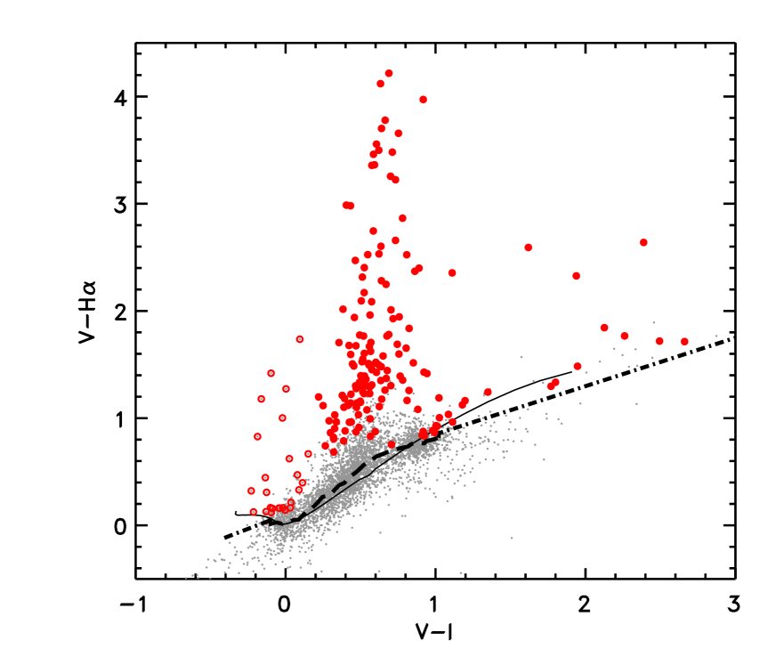
Figure 4.— Colour–colour diagram of the selected 4 156 stars in the field of SN 1987A. The dashed line represents the running median $V-H\alpha$ colour, obtained with a box-car size of 100 points, whereas the thin solid line shows the model atmospheres of Bessell et al. (1998). A total of 189 objects with a $V-H\alpha$ excess larger than $4\,\sigma$ are indicated with large dots.

A total of 189 objects, indicated by large dots in Figure 4, have a $V-H\alpha$ index exceeding that of the reference template at the same $V-I$ colour by more than four times the uncertainty on their $V-H\alpha$ values. These are the objects with a $V-H\alpha$ excess at the $4\,\sigma$ level and, as we shall see later, most of them are bona-fide PMS stars.

Figure 5.— Histogram of the H$\alpha$ luminosities of the 189 stars with H$\alpha$ excess at the $4\,\sigma$ level (dashed line) and of for the 133 bona-fide PMS that also have an emission $W_{\rm eq}(H\alpha)>10$ Å   and are not Ae/Be stars (solid line).

Since the contribution of the H$\alpha$ line to the $V$ magnitude is completely negligible, the magnitude $\Delta H\alpha$ corresponding to the excess emission is simply:

$$\Delta H\alpha=(V-H\alpha)^{\rm obs}-(V-H\alpha)^{\rm ref}$$ (2)

where the superscript obs refers to the observations and ref to the reference template. Once $\Delta H\alpha$ is determined in this way, the H$\alpha$ emission line luminosity $L(H\alpha)$ can be immediately obtained from the photometric zero point and absolute sensitivity of the instrumental set-up and from the distance to the sources. We have assumed a distance to the LMC and, more specifically, to SN 1987A of $51.4\pm 1.2$ kpc (Panagia et al. 1991, later updated in Panagia 1999), whereas the photometric properties of the instrument were taken from the WFPC2 Instrument Handbook (Heyer & Biretta 2004; namely inverse sensitivity PHOTFLAM$=1.461\times 10^{-16}$ and photometric zero-point ZP(Vegamag)$=17.564$). We derive a median value of the luminosity of the 189 objects with H$\alpha$ excess of $4\times 10^{31}$ erg/s or $10^{-2}$ L${}_{\odot}$. A histogram of the individual $L(H\alpha)$ values is shown in Figure 5 (dashed line).

It should be noted that, because of the width of the H$\alpha$ filter, $\Delta H\alpha$ includes a small contribution due to [NII] emission features at $6\,548$ Å  and $6\,584$ Å. Generally, their intensities do not exceed $1.2$ % and $3.5$ %, respectively, of the H$\alpha$ line intensity, and in many instances the [NII] doublet lines are much weaker, i.e. $<0.1\,\%$ of the H$\alpha$ line intensity (e.g. Edwards et al. 1987; Hartigan, Edwards & Ghandour 1995). These intensities should be even lower for PMS stars in the LMC because of the lower metallicity relative to the Milky Way. However, to take a conservative approach, we have simply adopted an average value that is half of the maximum for Galactic T-Tauri stars and we give as uncertainty half of the measured range. We will therefore adopt average values of $(1.8\pm 1.8)$ % and $(0.6\pm 0.6)$ % relative to the H$\alpha$ intensity, for the 6 584 Å   and 6 548 Å   [NII] lines, respectively (note that the uncertainties after the $\pm$ sign here are meant to show the entire span of the range, not just the $1\,\sigma$ value). Considering the width of the H$\alpha$ filter of the WFPC2, only the 6 548 Å   [NII] line contaminates the H$\alpha$ measurements, whereas for measurements made with the H$\alpha$ filter on board the ACS, both lines will be included (albeit only in part for the 6 548 Å   line). Although the resulting corrections on the H$\alpha$ intensity are quite small (namely $0.994$ for the WFPC2 F656N filter and $0.979$ for the ACS F658N filter, on average), they are systematic and it is therefore good practice to apply them in all cases.

Typically, the combined total uncertainty on our $L(H\alpha)$ measurements is $\sim 15\,\%$ and is completely dominated by the statistical uncertainty on the H$\alpha$ photometry. The systematic uncertainty on the distance to the field of SN 1987A accounts for 5 % (see Panagia 1999), whereas the typical uncertainty on the absolute sensitivity of the instrumental setup is of order 3 %.

3.2. The H$\alpha$ equivalent width

If the stars defining the reference template had no H$\alpha$ absorption features (we have established above that they do not have H$\alpha$ in emission), their $V-H\alpha$ index would correspond to that of the pure continuum and could then be used to derive the equivalent width of the H$\alpha$ emission line, $W_{\rm eq}(H\alpha)$. While this approximation might be valid for stars with a conspicuous H$\alpha$ emission, it is clearly not applicable in general. It is, however, possible in all cases to derive the level of the H$\alpha$ continuum by using properly validated models atmospheres.

As discussed above, the models of Bessell et al. (1998) reproduce quite reliably the observed broad-band colours (see e.g. Figure 2). This means that, even though the models might lack the resolution necessary to realistically reproduce spectral lines (hence the small discrepancy between the dashed line and the squares in Figure 3), the level of the continuum can be trusted. One can, therefore, fit the continuum in those models in a range containing the H$\alpha$ line (e.g. $6\,500-6\,620$ Å ) and fold the resulting “H$\alpha$-less” model spectra through the instrumental set-up (e.g. with Synphot), so as to derive the magnitude of the sole continuum in the H$\alpha$ band ($H\alpha^{c}$) as a function of spectral type or effective temperature. We present in the Appendix the relationships between $V$, $I$ and $H\alpha^{c}$ for several HST instruments and filters. The difference between the observed $H\alpha$ magnitude and $H\alpha^{c}$ provides a direct measure of $W_{\rm eq}(H\alpha)$, as we explain below.

We recall that the equivalent width of a line is defined as:

$$W_{\rm eq}=\int{(1-P_{\lambda})\,d\lambda}$$ (3)

where $P_{\lambda}$ is the profile of the line, or the spectrum of the source divided by the intensity of the continuum, and the integration is extended over the spectral region corresponding to the line. If the line profile is very narrow when compared to the width of the filter, i.e. if the line falls completely within the filter bandpass as is typical of emission lines, then $W_{\rm eq}(H\alpha)$ is simply given by the relationship:

$$W_{\rm eq}(H\alpha)=\mathrm{RW}\times[1-10^{-0.4\times(H\alpha-H\alpha^{c})}]$$ (4)

where $\mathrm{RW}$ is the rectangular width of the filter (similar in definition to the equivalent width of a line), which depends on the characteristics of the filter. Values of $\mathrm{RW}$ for the H$\alpha$ bands of past and current HST instruments are given in the Appendix (Table LABEL:tab4). As in the case of $L(H\alpha)$, the statistical uncertainty on the equivalent width is dominated by the uncertainty on the $H\alpha$ magnitude, typically of order 15 % in our selection. Moreover, the value of $W_{\rm eq}(H\alpha)$ obtained in this way is also subject to some systematic uncertainties produced by the model atmospheres used to interpolate the level of the continuum, such as e.g. metallicity, surface gravity or spectral resolution, and should therefore be taken with caution. On the other hand, we show in the Appendix that the equivalent widths (in absorption) obtained by applying this method to the high-resolution model spectra of Munari et al. (2005) are in excellent agreement with those obtained via standard spectro-photometry (see Figure LABEL:fig18).

Similarly, the values of $W_{\rm eq}(H\alpha)$ that we obtain in the field of SN 1987A are fully consistent with those of young PMS stars. In Figure 6 we show the value of $W_{\rm eq}(H\alpha)$ as a function of $V-I$ for the $4\,156$ selected stars. As mentioned earlier, there are 189 objects with a $\Delta H\alpha$ excess above the $4\,\sigma$ level and they are indicated as thick symbols (circles and triangles) in Figure 6. Since the equivalent width shown in Figure 6 is that of the pure emission component, the spectra of stars with small $W_{\rm eq}$, say $\lesssim 10$ Å, actually show an H$\alpha$ in absorption. For this reason, we conservatively ignore stars with measured $W_{\rm eq}(H\alpha)<10$ Å, since this value is about the largest absorption equivalent width expected for normal stars (see Figure LABEL:fig18 in the Appendix). A total of 164 objects satisfy this condition, but, in light of our conservative threshold, this must be considered as a lower-limit to the number of objects with genuine H$\alpha$ excess.

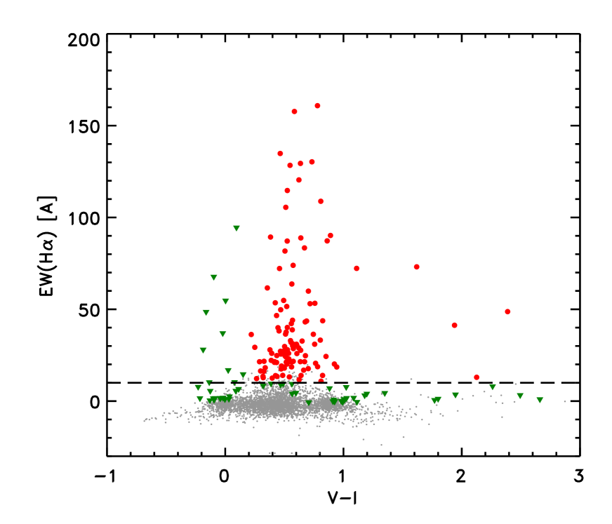
Figure 6.— Equivalent width of the selected 4 156 stars in the field of SN 1987A, as a function of their $V-I$ colour. Of the 189 stars with H$\alpha$ excess at the $4\,\sigma$ level (circles and triangles), a total of 164 have $W_{\rm eq}(H\alpha)>10$ Å. While objects bluer than $V-I\simeq 0.2$ are probably Ae/Be stars, there are 133 redder stars with significant H$\alpha$ excess (marked as circles) that we consider bona-fide low-mass PMS stars.

Values of $W_{\rm eq}(H\alpha)$ for the sample range from 10 Å  to 650 Å, with a median of 19 Å. These values are in excellent agreement with those obtained by Panagia et al. (2000) from the $R-H\alpha$ colour excess of the stars in this field and represent a refinement of those measurements, since these are based on a more accurate determination of the level of the continuum. These equivalent widths are typical of PMS stars (e.g. Muzerolle, Hartmann & Calvet 1998) and about two orders of magnitude smaller than those expected for pure nebular emission (see discussion in Section 6). While objects bluer than $V-I\simeq 0.2$ are probably Ae/Be stars, there are 133 redder stars with significant H$\alpha$ excess (marked as circles in Figure 6) that are most likely bona-fide low-mass PMS stars of various ages, as we will show in the following sections. A histogram of their H$\alpha$ luminosities is shown in Figure 5 (solid line).

4. Accretion luminosity and mass accretion rate

It is generally accepted (see e.g. Hartmann et al. 1998) that the energy $L_{\rm acc}$ released by the magnetospheric accretion process goes towards ionising and heating the circumstellar gas. In this hypothesis, the bolometric accretion luminosity $L_{\rm acc}$ can be determined from a measurement of the reradiated energy and, in particular, via the measured H$\alpha$ luminosity that is produced in the process.

In order to determine the exact relationship between $L(H\alpha)$ and $L_{\rm acc}$, we have used literature values of $L_{\rm acc}$ and $L(H\alpha)$ measurements as recently summarized by Dahm (2008) for PMS stars in the Taurus–Auriga association. As pointed out by Dahm himself, there may be a serious problem in determining an empirical relationship between $L_{\rm acc}$ and $L(H\alpha)$ measurements because the two quantities were determined from non-simultaneous observations. The intensity of the H$\alpha$ line from PMS sequence stars is known to vary by about 20 % on a time scale of a few hours and by as much as a factor of 2 – 3 in a few days (e.g. Fernandez et al. 1995; Smith et al. 1999; Alencar et al. 2001). For this reason, a relationship between $L(H\alpha)$ and $L_{\rm acc}$ is necessarily rather uncertain, although a very clear trend can be seen in the $L_{\rm acc}~{}vs.~{}L(H\alpha)$ plot shown by Dahm (2008). His logarithmic best fit would provide a slope of $1.18\pm 0.26$ for such a relationship. On the other hand, theoretical models (e.g. Muzerolle, Calvet & Hartmann 1998) would predict logarithmic slopes of about unity for low accretion rates, hence for faint H$\alpha$ luminosities, and shallower slopes for higher luminosities.

In the absence of compelling evidence in favour or against a steep slope, we will adopt a logarithmic slope of unity for the empirical $L_{\rm acc}~{}vs.~{}L(H\alpha)$ relationship, i.e. a constant ratio $L_{\rm acc}/L(H\alpha)$, and determine the proportionality constant from an elementary fit of the data summarised by Dahm (2008). On this basis we obtain:

$$\log L_{\rm acc}=(1.72\pm 0.47)+\log L(H\alpha)$$ (5)

As anticipated, the resulting uncertainty on $L_{\rm acc}$ is rather large, as high as a factor of 3, but this is the best one can obtain with the available data sets. In view of the convenience and the feasibility of determining $L_{\rm acc}$ from $L(H\alpha)$ for PMS outside our own Galaxy, it would be of paramount importance to obtain a proper calibration of the $L_{\rm acc}~{}vs.~{}L(H\alpha)$ relationshipby making simultaneous spectral observations of PMS stars over a suitably wide wavelength baseline, i.e. covering at least the range 3000–8000 Å, and possibly extending it to the near IR with measurements of Paschen and Brackett lines. High quality data of this type are already available for the Orion Nebula Cluster, collected by dedicated projects both from ground based observatories and with the HST (i.e. the Legacy Program on Orion; P.I. Massimo Robberto) and their analysis is in progress to provide a more accurate calibration of the $L_{\rm acc}~{}vs.~{}L(H\alpha)$ relationship (Da Rio et al., in preparation; Robberto et al., in preparation; Panagia et al., in preparation).

The median value of the accretion luminosity thus obtained for our sample of 133 PMS stars is $\sim 0.57$ L${}_{\odot}$, in good agreement with the value of $0.54$ L${}_{\odot}$ derived from the U-band excess measured by Romaniello et al. (2004) for stars in the same field, especially considering that their selection of stars with excess emission is less stringent than our $4\,\sigma$ level (we discuss this point in Section 7).

Once $L_{\rm acc}$ is known, the mass accretion rate follows from the free-fall equation that links the luminosity released in the impact of the accretion flow with the rate of mass accretion $\dot{M}_{\rm acc}$ according to the relationship:

$$L_{\rm acc}\simeq\frac{G\,M_{*}\,\dot{M}_{\rm acc}}{R_{*}}\left(1-\frac{R_{*}}{R_{\rm in}}\right)$$ (6)

where $G$ is the gravitational constant, $M_{*}$ and $R_{*}$ the mass and photospheric radius of the star and $R_{\rm in}$ the inner radius of the accretion disc. The value of $R_{\rm in}$ is rather uncertain and depends on how exactly the accretion disc is coupled with the magnetic field of the star. Following Gullbring et al. (1998), we adopt $R_{\rm in}=5\,R_{*}$ for all PMS objects.

As regards $R_{*}$, we derive it from the luminosity and effective temperature of the stars, which in turn come from the observed colour $(V-I)$ and magnitude ($V$), properly corrected for interstellar extinction as provided by Romaniello (1998), Panagia et al. (2000) and Romaniello et al. (2002). The adopted distance to SN 1987A is $51.4$ kpc (Panagia et al. 1991; Panagia 1999), as mentioned above. The stellar mass $M_{*}$ was estimated by comparing the location of a star in the Hertzsprung–Russell (H–R) diagram with the PMS evolutionary tracks. As for the latter, we adopted those of Degl’Innocenti et al. (2008; see also Tognelli, Prada Moroni & Degl’Innocenti, in preparation), for metallicity $Z=0.007$ or about one third $Z_{\odot}$, as appropriate for the LMC (e.g. Hill, Andrievsky, & Spite 1995; Geha et al. 1998). These new PMS tracks were specifically computed with an updated version of the FRANEC evolutionary code (see Chieffi & Straniero 1989 and Degl’Innocenti et al. 2008 for details and Cignoni et al. 2009 for an application). However, in order to assess how differences in the evolutionary models affect our results, in Section 6.1 we also consider PMS tracks from other authors, namely those of D’Antona & Mazzitelli (1997) and Siess, Dufour & Forestini (2000).

Figure 7.— Distribution of the mass accretion rates of the 133 bona-fide PMS stars. Note that 9 objects with $\dot{M}_{\rm acc}>10^{-7}$ M${{}_{\odot}}$  yr${}^{-1}$ are not shown in the graph.

Combining Equations 5 and 6, we can link the mass accretion rate $\dot{M}_{\rm acc}$, in units of M${{}_{\odot}}$ yr${}^{-1}$, to $L(H\alpha)$:

$$\log\frac{\dot{M}_{\rm acc}}{M_{\odot}{\rm yr}^{-1}} = -7.39+\log\frac{L_{\rm acc}}{L_{\odot}}+\log\frac{R_{*}}{R_{\odot}}-\log\frac{M_{*}}{M_{\odot}}$$

$$= (-5.67\pm 0.47)+\log\frac{L(H\alpha)}{L_{\odot}}+\log\frac{R_{*}}{R_{\odot}}-\log\frac{M_{*}}{M_{\odot}}$$

The distribution of mass accretion rates found in this way for the 133 PMS stars in our sample is shown in Figure 7. The median value of $2.9\times 10^{-8}$ M${{}_{\odot}}$  yr${}^{-1}$ is in remarkably good agreement with the median rate of $2.6\times 10^{-8}$ M${{}_{\odot}}$  yr${}^{-1}$ found by Romaniello et al. (2004) from the U-band excess.

The uncertainty on $\dot{M}_{\rm acc}$ is dominated by the approximate knowledge of the ratio of $L_{\rm acc}$ and $L(H\alpha)$ in Equation 5. As explained above, empirical measurements and theoretical models suggest a value of $L_{\rm acc}/L(H\alpha)\simeq 52$ but with an uncertainty of a factor of three. Since the ratio, however, is the same for all stars, the comparison between different objects is not hampered by this uncertainty, as long as the statistical errors are small.

As for the other quantities in Equation 7, we discuss here the sources of statistical uncertainty, while systematic errors are addressed separately in Section 6. With our selection criteria, the typical uncertainty on $L(H\alpha)$ is 15 % and is dominated by random errors. The uncertainty on $R_{*}$ is typically 7 %, including a 5 % systematic uncertainty on the distance modulus. As for the mass $M_{*}$, since it is determined by comparing the location of a star in the H–R diagram with evolutionary tracks, both systematic and statistical uncertainties are important. The uncertainty on the temperature is mostly statistical and of order 3 %, while that on the luminosity is $7\,\%$, comprising both random errors (1 % uncertainty on the bolometric correction and 3 % on the photometry) and systematic effects (5 % uncertainty on the distance modulus). When we interpolate through the PMS evolutionary tracks to estimate the mass, the uncertainties on $T_{\rm eff}$ and $L$ imply an error of $\sim 7\,\%$ on $M_{*}$. However, an even larger source of systematic uncertainty on $M_{*}$ comes from the evolutionary tracks, as we explain in Section 6. In summary, the combined statistical uncertainty on $\dot{M}_{\rm acc}$ is 17 %.

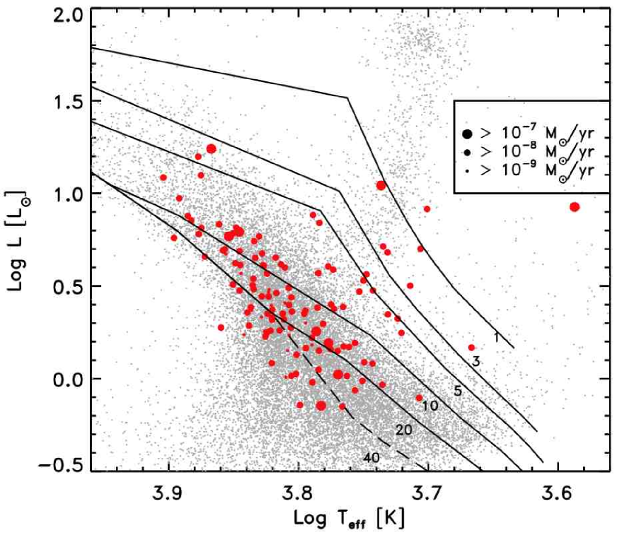
Figure 8.— Location of the bona-fide PMS candidates in the H–R diagram, compared with the isochrones of Degl’Innocenti et al. (2008) for metallicity $Z=0.007$ (the ages, in Myr, are indicated next to each isochrone). The size of the symbols is proportional to the mass accretion rate $\dot{M}_{\rm acc}$ (see legend).

5. Ages of PMS stars

Having identified a population of bona-fide PMS stars, with well defined accretion luminosities and mass accretion rates, it is instructive to place them in the H–R diagram. We do so in Figure 8 where bona-fide PMS stars are marked as large dots, with a size proportional to their $\dot{M}_{\rm acc}$ value, according to the legend. Also shown in the figure are the theoretical isochrones from the FRANEC models of Degl’Innocenti et al. (2008) for $Z=0.007$ and ages as indicated (in units of Myr, from the stellar birth line; see Palla & Stahler 1993). The dashed line, corresponding to a 40 Myr isochrone, defines in practice the zero-age main sequence (MS).

It is noteworthy that the majority of PMS objects in Figure 8 are rather close to the MS and would have easily been missed if no information on their H$\alpha$ excess had been available. Indeed, it is customary to identify PMS stars in a colour–magnitude diagram by searching for objects located above and to the right of the MS, since this is where one would expect to find very young objects. This method was first used by Gilmozzi et al. (1994) to identify a population of PMS stars outside the Milky Way, namely in the LMC cluster NGC 1850. More recent applications of this method include e.g. those of Sirianni et al. (2000), Nota et al. (2006) and Gouliermis et al. (2006).

Unfortunately, this method of identification is not very reliable, since the existence of an age spread and the presence in the same field of a considerably older population, as well as unaccounted patchy absorption, all tend to fill up the parameter space between the MS and the birth line, thereby thwarting any attempts to identify PMS stars on the basis of their effective temperature and luminosity alone. In the specific case of the SN 1987A field studied here, Panagia et al. (2000) have shown that the age spread is remarkable, with several generations of young stars with ages between 1 and 150 Myr superposed on a much older field population ($0.6-6$ Gyr). In such circumstances, as Figure 8 shows, broad-band photometry alone would have not identified as such most of our bona-fide PMS stars.

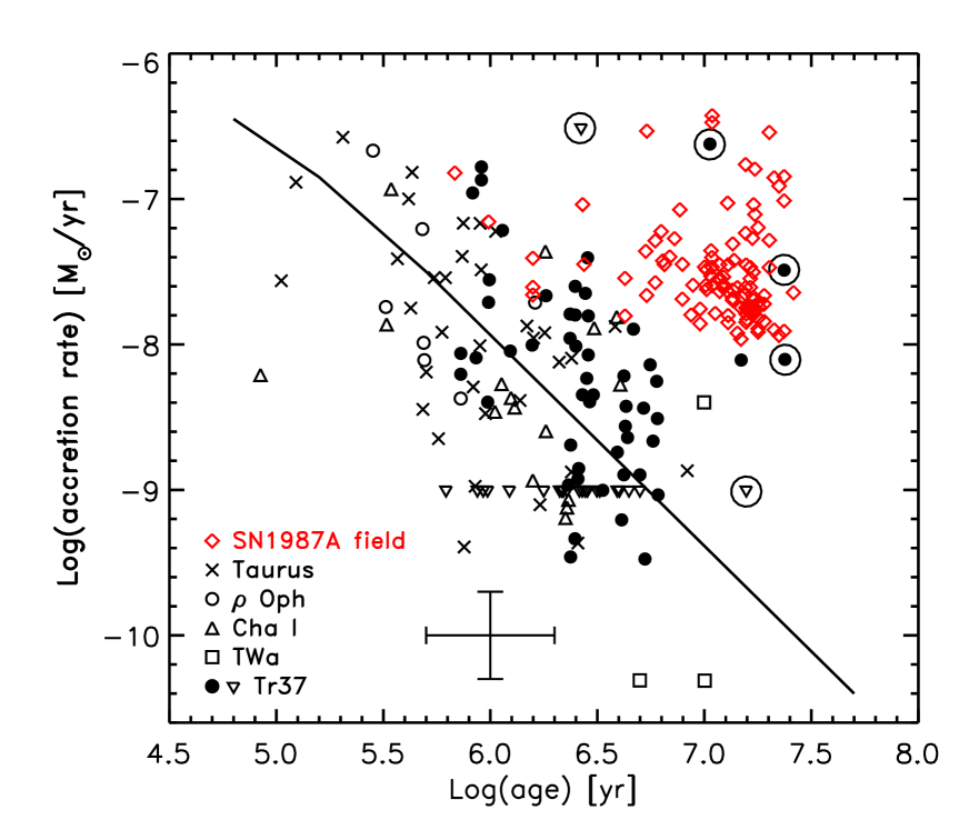
Figure 9.— The mass accretion rate as a function of stellar age for our bona-fide PMS stars (diamonds) is compared here with that of a similar number of Galactic T Tauri stars (see legend) from the work of Sicilia–Aguilar et al. (2006), from whom all Galactic data-points are taken (the large cross indicates the uncertainties as quoted in that paper). The solid line shows the evolution for current models of viscous disc evolution from Hartmann et al. (1998). Our measurements are systematically higher than the models, but are in agreement with the $\dot{M}_{\rm acc}$ values of G type stars in the Galaxy (large circles).

In accordance with their proximity to the MS, the majority of bona-fide PMS stars turn out to be relatively old. The ages of individual objects were determined by interpolating between the isochrones in the H–R diagram. They range from 1 to $\sim 50$ Myr, with a median age of $13.5$ Myr, in very good agreement with the estimated age of both SN 1987A and its nearby Star 2 of $\leq 13$ Myr (see Scuderi et al. 1996 and references therein). Panagia et al. (2000) find that about 35 % of the stars younger than 100 Myr in this field have a typical age of 12 Myr, again consistent with the estimated age of the bona-fide PMS stars.

The relatively old age of our PMS stars might appear at odds with the rather large mass accretion rates that we obtain for that population, namely $\sim 10^{-8}$ M${{}_{\odot}}$  yr${}^{-1}$. According to current models of viscous disc evolution (see Hartmann et al. 1998; Muzerolle et al. 2000), the mass accretion rate of a $\sim 14$ Myr old PMS population should be of order $3\times 10^{-10}$ M${{}_{\odot}}$  yr${}^{-1}$. Those models, shown in Figure 9 as a solid line, adequately reproduce the trend of decreasing $\dot{M}_{\rm acc}$ with stellar age observed for very low-mass Galactic T-Tauri stars (see e.g. Calvet et al. 2004), but under-predict our measurements (indicated by diamonds) by over an order of magnitude.

On the other hand, recent observations of PMS stars in the cluster Trumpler 37 by Sicilia–Aguilar et al. (2006), from whom the data-points in Figure 9 are taken, indicate that the value of $\dot{M}_{\rm acc}$ for $\sim 10-20$ Myr old G-type PMS stars (large circles) is considerably larger, indeed of order $\sim 10^{-8}$ M${{}_{\odot}}$  yr, in excellent agreement with our results. With a median mass of $1.2$ M${{}_{\odot}}$ and a median $V-I$ colour of $0.56$, our bona-fide PMS stars are fully consistent with the G spectral type and suggest that stars of higher mass have a higher $\dot{M}_{\rm acc}$ value at all ages. As mentioned in the Introduction, Muzerolle et al. (2003; 2005), Natta et al. (2004; 2006) and Calvet et al. (2004) suggest a dependence of the type $\dot{M}_{\rm acc}\propto M^{2}$ from the analysis of a sample of low-mass and intermediate-mass T-Tauri stars, albeit with a large uncertainty on the index (see also Clarke & Pringle 2006). A similar trend is proposed by Sicilia–Aguilar et al. (2006), yet with even lower statistical significance due to the limited mass range covered by their observations. The range of masses that we cover here is also quite limited and does not allow us to address this issue in detail. We will, however, do so in a forthcoming paper (De Marchi et al. 2008, in preparation), where we compare the accretion rates in this field with those of a much younger and an order of magnitude more numerous population of PMS stars in the Small Magellanic Cloud. While in the SN 1987A field the detection limits imposed by the WFPC2 photometry do not allow us to reach stars with mass below $\sim 0.9$ M${}_{\odot}$, in that paper, based on ACS observations, we will study stars down to $\sim 0.4$ M${}_{\odot}$.

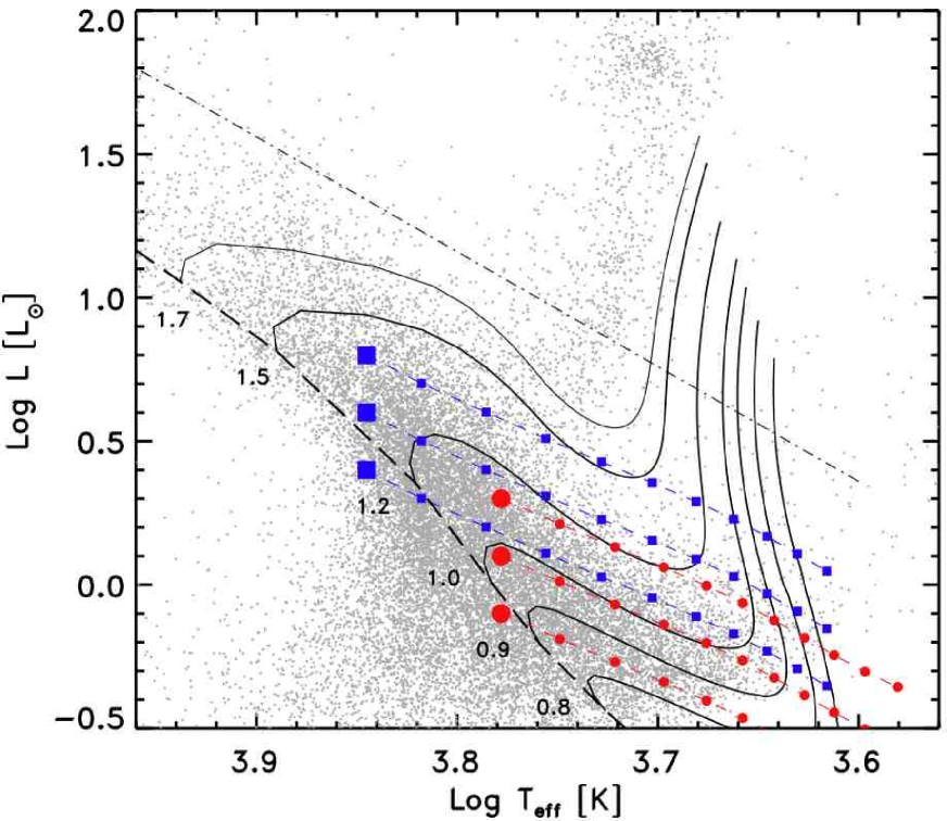
Figure 10.— Simulated effects of a reddening increase on the mass determination via interpolation through the evolutionary tracks. The solid lines are the track of Siess et al. (2000) corresponding to the masses as indicated. Small circles and squares show the reddening displacement, from the unreddened locations (larger circles and squares), in increments of $E(V-I)=0.1$ according to the extinction law of Scuderi et al. (1996) for this field. The dot-dashed line indicates the line of constant radius, while the thick dashed line is the same 40 Myr isochrone as in Figure 8.

6. Systematic errors

The main sources of systematic uncertainty on the derived mass accretion rates are (i) discrepancies in the isochrones and evolutionary tracks, (ii) reddening, (iii) H$\alpha$ emission generated by sources other than the accretion process, and (iv) the contribution of the nebular continuum to the colours of the stars. We discuss all these effects in this section.

6.1. Models of stellar evolution

As explained in Sections 4 and 5, the mass and age of PMS stars are determined by interpolation of their location in the H–R diagram, using model evolutionary tracks and isochrones as references. Apart for possible inaccuracies in the models input physics and errors in the interpolation, the largest source of systematic uncertainty on the derived mass and age comes from the use of models that might not properly describe the stellar population under study (e.g. because of the wrong metallicity) and from differences between models of various authors.

For instance, if we had used Siess et al.’s (2000) tracks for metallicity 1/2 solar in place of those for 1/3 solar, the masses of our PMS objects would be systematically higher by about 20 %. For metallicity 1/2 solar, using the tracks of Siess et al. (2000) or those of D’Antona & Mazzitelli (1997) results in masses that agree to within a few percent. On the other hand, when it comes to the determination of the age, using D’Antona & Mazzitelli’s (1997) isochrones one would derive ages twice as young for stars colder than $\sim 6\,500$ K, while for hotter stars ages would only be 20 % lower.

In summary, systematic uncertainties of order 20 % are to be expected for the mass and possibly higher for the age determination.

6.2. Reddening

Dust extinction systematically displaces stars in the H–R diagram towards lower luminosities and effective temperatures. This is shown graphically in Figure10, for six model stars, three with $T_{\rm eff}=6\,000$ K (large circles) and three with $T_{\rm eff}=7\,000$ K (large squares). The effects of a reddening increase from $E(V-I)=0$ to $E(V-I)=1$ on the location of the stars in the H–R diagram is shown by the smaller symbols, corresponding to increments of $E(V-I)=0.1$. We have adopted here the extinction law as measured specifically in the field of SN 1987A by Scuderi et al. (1996).

Since the reddening vector in the H–R plane is almost parallel to the lines of constant radius (as shown by the dot-dashed line for $R=10$ R${}_{\odot}$), extinction affects only marginally the estimate of the stellar radius. However, at low temperatures the reddening vector crosses the evolutionary tracks (solid lines), thus leading to an underestimate of the stellar mass, if no extinction correction is applied. In turn, this will result in a systematically higher value of the $R_{*}/M_{*}$ ratio and, therefore, in an overestimate of the mass accretion rate derived via Equation 6.

In order to better gauge the uncertainty on the value of $R_{*}/M_{*}$ caused by unaccounted extinction, we have determined the mass and radius of each one of the artificially reddened model stars shown in Figure 10, in exactly the same way in which we did that for bona-fide PMS stars, and compared those with the known input values. The result is shown graphically in Figure 11, where, the relation between the derived and input $R_{*}/M_{*}$ ratios is shown as a function of colour excess $E(V-I)$.

Regardless of the input parameters ($L$, $T_{\rm eff}$ or $R_{*}/M_{*}$), it appears that over the range explored here the derived $R_{*}/M_{*}$ ratio increases slowly with colour excess (see dashed line that best fits the median values indicated by the crosses). In particular, underestimating the $E(V-I)$ colour excess by $\sim 0.4$ mag would lead to a 30 % overestimate of $R_{*}/M_{*}$ (and hence of $\dot{M}_{\rm acc}$). This appears unlikely, considering that the best estimate of the total extinction — including the Milky Way component — towards Star 2, one of the two bright close companions to SN 1987A, is $E(V-I)=0.21$ (Scuderi et al. 1996), with a $1\,\sigma$ dispersion over the field of $\sim 0.07$ (Romaniello 1998; Panagia et al. 2000). According to Zaritsky et al. (2004), the average reddening towards cool (5500 K$<T_{\rm eff}<$6 500 K) stars in the LMC is $A_{\rm V}=0.43$, thus implying $E(V-I)\simeq E(B-V)\simeq 0.14$. Therefore, for an average LMC star forming region, omitting the extinction correction would result in a 10 % overestimate of the mass accretion rate. This error, albeit systematic, is smaller than most other systematic uncertainties and comparable to the measurement errors.

Nonetheless, we would like to stress here that the effects of patchy absorption can be more severe in regions of high extinction. Therefore, whenever possible, one should apply extinction corrections to each individual stars, as it was done for the photometric catalogue of Romaniello et al. (2002) that we use here.

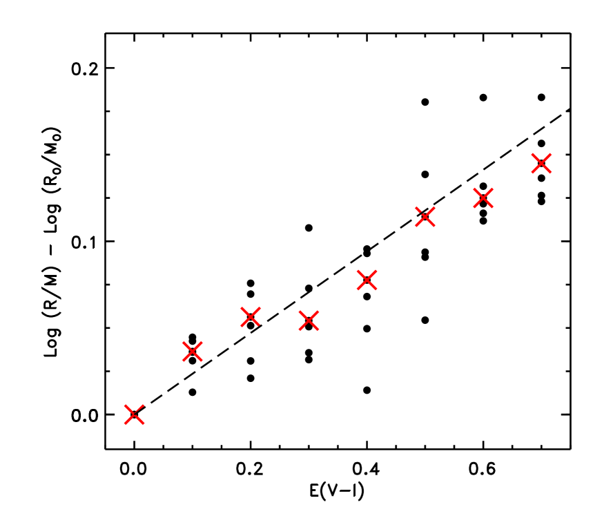
Figure 11.— Overestimate of the $R/M$ ratio as a function of $E(V-I)$ when the extinction remains unaccounted. Thick dots represent the $R/M$ ratios of the artificially reddened stars (see Figure 10) and the crosses their median values.

6.3. H$\alpha$ emission not due to the accretion process

The underlying assumption in the determination of the mass accretion rate of PMS stars is that the gravitational energy $L_{\rm acc}$ released in the accretion process goes into heating of the gas at the boundary layer (see e.g. Hartmann et al. 1998). In this case, the luminosity of the H$\alpha$ emission line can provide a measure of the accretion energy, because it acts as a natural “detector” of the luminosity released in the accretion process.

Thus, the issue to address is whether the measured $L(H\alpha)$ is produced only and entirely as a result of the energy released in the accretion process. Obviously, depending on the geometry and orientation of the circumstellar disc and on the specifics of the accretion process, some of the ionising energy could escape without effectively ionising the local gas. This would result in an underestimate of the true mass accretion rate for some stars, but this is true of any method that uses H emission lines as indicators of the accretion process and, therefore, it does not affect the comparison of our results with those of others (see Figure 9).

One possibility that we can readily exclude is that the H$\alpha$ emission that we detect is due to chromospheric activity. The total chromospheric emission of a solar-type star on the subgiant branch corresponds to a luminosity of about $10^{-4}$ L${}_{\odot}$ (Ulmschneider 1979; Pasquini et al. 2000), i.e. two orders of magnitude less than what we measure.

On the other hand, we must also consider the possibility that H$\alpha$ emission might occur in discrete H knots along the line of sight, in places unrelated with the PMS object. Furthermore, hot nearby massive stars may ionise the H gas in which PMS stars are immersed, eventually producing H$\alpha$ emission when the gas recombines. Both these effects would result in a overestimate of $\dot{M}_{\rm acc}$, but we show below that the probability of this happening is very small.

As for intervening H$\alpha$ emission along the line of sight, it would have to arise in knots of ionised H, e.g. very compact HII regions, contained within our photometric apertures. However, if such knots exist, they should not project only against stars and, therefore, narrow-band images should reveal H$\alpha$ emission where broad-band imaging shows no or very low signal (see Section 6.3). Since this is not observed, statistical arguments rule out this possibility as a significant source of the observed H$\alpha$ excess emission.

While it is possible that some of the H$\alpha$ emission that we detect is due to diffuse nebular emission in the HII region not powered by the accretion process, if the emission is extended and uniform over an area of at least $0\farcs 5$ radius around the star its contribution cancels out with the rest of the background when we perform aperture photometry (using an aperture of $0\farcs 2$ radius for the object and an annulus of $0\farcs 3-0\farcs 5$ for the background). The subtraction would not work if the emission were not uniform, as for example in the case of a filament that projects over the star but that does not cover completely the background annulus. However, we have visually inspected all objects with excess H$\alpha$ emission and excluded the few cases where a spurious filament of this type could be seen (see Romaniello 1998; Panagia et al. 2000).

Another case in which the emission does not cancel out is when the gas ionised by an external source is associated to the star and completely contained within our photometric aperture. We recall here that the typical size of a circumstellar disc is of order 100 AU (e.g. Hartmann et al. 1998), or about $0.02$ pixel at the distance of SN 1987A, and that the median $L(H\alpha)$ that we measure for our PMS stars is $4\times 10^{31}$ erg s${}^{-1}$, or about $10^{-2}$ L${}_{\odot}$ (see Figure 5). We can then calculate how close a PMS stars should be to a hot, UV-bright star for the latter to flood the PMS circumstellar disc with enough ionising radiation to cause at least 10 % of the H$\alpha$ luminosity that we measure from that source.

Let $r=100$ AU be the external radius of the circumstellar disc and $d$ the distance to an ionising star that illuminates the disc, assumed to have zero inclination (i.e. face on), so that $\phi=r^{2}/(4\,d^{2})$ is the solid angle subtended by the disc. Let $\beta_{2}$ be the recombination coefficient to the first excited level in an optically thick H gas. If $V$ is the volume of the gas and $n_{e}$ and $n_{p}$ are the electron and proton densities per unit volume, the global ionisation equilibrium equation (case B; see Baker & Menzel 1938) is then:

$$N_{L}\,\phi=\beta_{2}\,n_{e}\,n_{p}\,V$$ (8)

where $N_{L}$ is the rate of ionising photons produced by the external star. Denoting with $\alpha_{3,2}$ the H$\alpha$ emission coefficient for the same gas, the luminosity of the H$\alpha$ recombination line can be written as:

$$L(H\alpha)=\alpha_{3,2}\,n_{e}\,n_{p}\,V$$ (9)

which allows us to express the luminosity of the H$\alpha$ emission caused by the external star as a function of its ionising photon rate $N_{L}$:

$$L^{\rm ext}(H\alpha)=\alpha_{3,2}/\beta_{2}\,N_{L}\,\phi.$$ (10)

The minimum distance beyond which the contribution of the ionising star to the total H$\alpha$ emission becomes negligible (i.e. 10 % or less) is given by:

$$d^{2}_{\rm min}=\frac{r^{2}}{4}\,\frac{\alpha_{3,2}}{\beta_{2}}\,\frac{10\,N_{L}}{L(H\alpha)}.$$ (11)

Table 1 gives the value of $\phi$ for a typical H$\alpha$ luminosity of $10^{-2}$ L${}_{\odot}$, as a function of the spectral type of the ionising star. Here we have used the compilation of Panagia (1973) for the appropriate stellar parameters. The table also provides the minimum distance $d_{\rm min}$ in pc and in arcsec (at the distance of SN 1987A) for a circumstellar disc of radius $r=100$ AU. We recall here that 1 arcsec corresponds to 10 WFPC2 pixels. The brightest star in the field studied here is an object with $\log T_{\rm eff}=4.7$ and $\log(L/L_{\odot})=5.8$, with an implied mass of $\sim 60$ M${{}_{\odot}}$ and an age less than 1 Myr (see Panagia et al. 2000). The corresponding value of $N_{L}$, from Panagia (1973), is $4\times 10^{49}$ s${}^{-1}$, thus implying $d_{\rm min}=0.95$ pc or 38 WFPC2 pixel for a gas temperature of 10 000 K. A careful inspection of the images shows that none of our candidate bona-fide PMS stars falls closer to this star than $d_{\rm min}$. The same applies to the second and third brightest stars in the field, respectively with $\log T_{\rm eff}=4.7$, $\log(L/L_{\odot})=5$ and $\log T_{\rm eff}=4.67$, $\log(L/L_{\odot})=4.75$, as well as to all fainter objects.

Table 1Possible effects of nearby ionising stars

SpT	$T_{\rm eff}$	$\log(L/L_{\odot})$	$\log N_{L}$	$\phi$	$d_{\rm min}$
	(K)		(s${}^{-1}$)		(pc)	($\arcsec$)
O4	50 000	6.11	49.93	3.42e-08	1.31	5.26
O6	42 000	5.40	49.08	2.43e-07	0.49	1.97
O7	36 500	4.81	48.62	6.93e-07	0.29	1.17
O9	34 500	4.66	48.08	2.43e-06	0.16	0.62
B0	30 900	4.40	47.36	1.27e-05	0.07	0.27
B1	22 600	3.72	45.29	1.50e-03	0.01	0.03

Note. — The values of $\phi$ and $d_{\rm min}$ are given for a 100 AU circumstellar H disc with a temperature of 10 000 K. For gas temperatures of 5 000K and 20 000 K the value of $\phi$ is respectively higher and lower by $7.5\,\%$, while $d_{\rm min}$ is $3.6\,\%$ larger and smaller, respectively.

It is convenient to calculate, for each PMS object, the total H$\alpha$ luminosity $L^{\rm ext}(H\alpha)$ caused by all neighbouring ionising stars, expressed as:

$$L^{\rm ext}(H\alpha)=\frac{r^{2}}{4}\,\frac{\alpha_{3,2}}{\beta_{2}}\,\sum_{i=1}^{N}\frac{(N_{L})_{i}}{d_{i}^{2}}$$ (12)

where $(N_{L})_{i}$ is the ionising photon rate of star $i$ and $d_{i}$ is its distance from the PMS object being considered. Besides the three brightest stars mentioned above, we have included as potential sources of the detected H$\alpha$ emission an additional 12 stars in the field with $\log T_{\rm eff}\geq 4.4$ and $\log(L/L_{\odot})\geq 4$, as classified by Romaniello et al. (2002). We note that these estimates of $L^{\rm ext}(H\alpha)$ are firm upper limits because we are assuming that (i) all disks are face-on relative to the hot stars, and that (ii) the projected distances on the sky are indeed the actual distances from the hot stars. The values of $L^{\rm ext}(H\alpha)$ obtained in this way for the 133 bona-fide PMS stars span the range $10^{-6}-10^{-4}$ L${}_{\odot}$, or typically three orders of magnitude less than the median PMS H$\alpha$ luminosity, as shown by the histogram in Figure 12. We can, therefore, conclude that in this specific field the contribution of hot ionising stars to the measured excess H$\alpha$ emission is negligible. We must stress, however, that the effect might be much more pronounced in younger star forming regions, such as the Orion Nebula or 30 Dor.

Figure 12.— Histogram of the ratio of observed and external H$\alpha$ luminosity for our bona-fide PMS stars. The observed H$\alpha$ luminosity is typically three to four orders of magnitude larger than the contribution due to external sources.

6.4. Nebular continuum

Finally, consideration must be given to the role of the nebular continuum, i.e. radiation caused by bound–free and free–free transitions in the gas and unrelated to the stellar photosphere. If present, nebular continuum will add to the intrinsic continuum of the star, thereby affecting both the observed total level and the slope. This could ultimately alter the measured broad-band colours of the source, thereby thwarting our attempts to infer the level of the continuum in the H$\alpha$ band from the observed $V$ and $I$ magnitudes. It is important to estimate the magnitude of this effect, as our method relies on the intrinsic $V-I$ colour of a star to derive its $\Delta H\alpha$ (see Equation 2).

Fortunately, the contribution of the nebular continuum appears to be insignificant. To prove this, we have assumed a fully ionised gas of pure H, considering only bound–free and free–free transitions and ignoring the contribution to the continuum from two-photon emission (Spitzer & Greenstein 1951). Using Osterbrock’s (1989, Chapter 4) tabulations, we find H$\alpha$ line intensity and H$\alpha$ continuum fluxes of the nebular gas as shown in Table 2, for gas electron temperatures in the range 5 000 K – 20 000 K. The purely nebular $W_{\rm eq}(H\alpha)$ ranges from $5\,000$ Å   to $9\,000$ Å, or two orders of magnitude higher than what we measure for PMS objects. We can, therefore, safely conclude that the nebular contribution to the continuum is negligible (less than 1 %).

Furthermore, we find that for gas temperatures in the range 5 000 K – 10 000 K the $V-I$ colour of the nebular continuum varies from $1.4$ to $0.5$, spanning a range typical of G–K type stars. Thus the effects of the nebular continuum on the $V-I$ colour of PMS stars remains insignificant even for the objects with the highest $W_{\rm eq}(H\alpha)$ in our sample.

Table 2Nebular emission and continuum of fully ionised H gas

$T_{\rm el}$	$F_{\nu}$	$F_{\lambda}$	$E(H\alpha)$	$W_{\rm eq}(H\alpha)$
5 000 K	$10.28\,10^{-40}$	$7.16\,10^{-29}$	$6.71\,10^{-25}$	9378 Å
10 000 K	$7.56\,10^{-40}$	$5.26\,10^{-29}$	$3.56\,10^{-25}$	6763 Å
20 000 K	$5.51\,10^{-40}$	$3.83\,10^{-29}$	$1.83\,10^{-25}$	4764 Å

Note. — $F_{\nu}$, $F_{\lambda}$ and $E(H\alpha)$ are given here in erg cm${}^{3}$ s${}^{-1}$ Hz${}^{-1}$, i.e. per unit volume ($V$), unit electron density ($n_{e}$) and unit proton density ($n_{p}$). The luminosity can be derived by multiplying the values listed here by $V\,n_{e}\,n_{p}$.