Large-Scale Outflows from AGN: a link between central black holes and galaxies

Abstract

We summarize the results from numerical simulations of mass outflows from AGN. We focus on simulations of outflows driven by radiation from large-scale inflows. We discuss the properties of these outflows in the context of the so-called AGN feedback problem. Our main conclusion is that this type of outflows are efficient in removing matter but inefficient in removing energy.

1 Introduction

AGN produce the powerful outflows of the electromagnetic radiation that in tunr can drive outflows of matter. These outflows and the central location of AGN in their host galaxies imply that AGN can play a key role in determining the physical conditions in the central region of the galaxy, the galaxy as a whole, and even intergalactic scales (e.g., Ciotti & Ostriker 1997, Ciotti et al. 2009; Sazonov et al. 2005; Springel et al. 2005; Fabian et al. 2006; Merloni & Heinz 2008, and references therein).

Outflows from AGN are an important link between the central and outer parts of the galaxy because AGN are powered by mass accretion onto a super massive black hole (SMBH). Thus the SMBH ’knows’ about the galaxy through the accretion flow whereas the galaxy knows about the SMBH through the outflows powered by accretion. To quantify this connection, let us express the radiation luminosity due to accretion as

$$L_{\mathrm{a}}=\epsilon_{\mathrm{r}}c^{2}\dot{M}_{\mathrm{a}},$$ (1)

where we invoke the simplest assumption such that the luminosity is proportional to the mass accretion rate ($\dot{M}_{\mathrm{a}}$) and a radiative (or the rest-mass conversion) efficiency ($\epsilon_{\mathrm{r}}$).

To estimate $\dot{M}_{\mathrm{a}}$, one often adopts the analytic formula by Bondi (1952) who considered spherically symmetric accretion from a non-rotating polytropic gas with uniform density $\rho_{\infty}$ and sound speed $c_{\infty}$ at infinity. Under these assumptions, a steady state solution to the equations of mass and momentum conservation exists with a mass accretion rate of

$$\dot{M}_{\mathrm{B}}=\lambda\,4\pi r^{2}_{\mathrm{B}}\rho_{\infty}c_{\infty},$$ (2)

where $\lambda$ is a dimensionless parameter that, for the Newtonian potential, depends only on the adiabatic index, $\gamma$ (cf. Bondi 1952). The Bondi radius, $r_{\mathrm{B}}$, is defined as

$$r_{\mathrm{B}}=\frac{GM}{c^{2}_{\infty}}$$ (3)

where $G$ is the gravitational constant and $M$ is the mass of the accretor.

To quantify AGN feedback, one can measure its efficiency in changing the flow of mass, momentum, and energy. The mass feedback efficiency $\epsilon_{\mathrm{m}}$ is defined as the ratio of the mass-outflow rate at the outer boundary $\dot{M}_{\mathrm{out}}$ to the mass-inflow rate at the inner boundary $\dot{M}_{\mathrm{in}}$, i.e.,

$$\epsilon_{\mathrm{m}}=\dot{M}_{\mathrm{out}}/\dot{M}_{\mathrm{in}}\,.$$ (4)

Here, we consider only the energy and momentum carried out by matter. Therefore, the momentum feedback efficiency ($\epsilon_{\mathrm{p}}$) is defined as the ratio of the total wind momentum $p_{\mathrm{w}}$ to the total radiation momentum ($L_{\mathrm{a}}/c$), i.e.,

$$\epsilon_{\mathrm{p}}=p_{\mathrm{w}}/\left(L_{\mathrm{a}}/c\right)\,.$$ (5)

Finally, the total energy feedback efficiency $\epsilon_{\mathrm{t}}$ is defined as the ratio between the sum of the kinetic power (kinetic energy flux) $P_{\mathrm{k}}$ and thermal energy power (thermal energy flux) $P_{\mathrm{th}}$ and the accretion luminosity of the system $L_{\mathrm{a}}$ (Eq. [1]), i.e.,

$$\epsilon_{\mathrm{t}}=\left(P_{\mathrm{k}}+P_{\mathrm{th}}\right)/L_{\mathrm{a}}\,,$$ (6)

where

$$\epsilon_{\mathrm{k}}=P_{\mathrm{k}}/L_{\mathrm{a}}$$ (7)

and

$$\epsilon_{\mathrm{th}}=P_{\mathrm{th}}/L_{\mathrm{a}}\,,$$ (8)

It follows that $\epsilon_{\mathrm{t}}=\epsilon_{\mathrm{k}}+\epsilon_{\mathrm{th}}$.

Several very sophisticated simulations of feedback effects were recently performed, e.g., Springel et al. (2005) (SDH05 hereafter), Di Matteo et al. (2005), and Booth & Schaye (2009) (BS09 hereafter). These simulations follow merging galaxies in which many processes were included, for example, star formation, radiative cooling in a complex multi-phase medium, BH accretion and feedback. In addition, these local and global processes were connected. However, all of this was possible at the cost of crude phenomenological realizations of some processes and the spatial resolution at a level larger than $r_{\mathrm{B}}$. Consequently, the efficiencies were assumed instead of being computed.

A main result of these simulations is that the famous $M_{\mathrm{BH}}-\sigma$ relation (e.g., Ferrarese & Merritt 2000; Gebhardt et al. 2000; Tremaine et al. 2002) was reproduced. In addition, the BH mass is little affected by the details of star formation and supernova feedback.

This is a great success of the current cosmological simulations models. However, as pointed out above (see also others e.g., Begelman & Nath 2005) the key feedback processes in the models represent “subgrid” physics. Therefore, in these cosmological and galaxy merger simulations AGN feedback cannot be directly related to AGN physics.

On the other hand, models that aim to provide insights to AGN physics do not include galaxy but rather focus on $r_{\mathrm{B}}$ or even smaller scales (e.g., Proga 2007; Proga et al. 2008; Kurosawa & Proga 2008; Kurosawa & Proga 2009a, b). Thus they cannot be directly related to AGN feedback on large scales. However, these smaller scale simulations can be used directly to measure the feedback efficiencies and in turn to quantify the effects that are assumed or parametrized in large scale simulations.

Here, we summarize the main findings from Kurosawa et al. (2009) where we attempted to determine if AGN can supply energy in the form and amount required by the cosmological and galaxy merger simulations. Our approach was to measure $\dot{M}_{\mathrm{a}}$, and various feedback efficiencies based on direct simulations of inflows and outflows in AGN, on sub-parsec and parsec scales performed by Kurosawa & Proga (2009b) (KP09 hereafter).

2 AGN Models in Recent Cosmological Simulations

Before we present our results, we briefly summarize what is required by the cosmological and galaxy merger simulations.

2.1 Mass Accretion Rates

As we mentioned above, cosmological and galaxy merger simulations (e.g., SDH05; Sijacki et al. 2007; BS09), the actual physical process of the mass-accretion onto the BH is not explicitly modeled because of a relatively poor resolution. These simulations rely on a separate analytical model to describe the small scale processes. The unresolved accretion process is usually described by a Bondi-Hoyle-Little formulation (e.g., Bondi 1952).

One can illustrate some important issues related to numerical realization of this process by considering a simpler Bondi accretion problem. Then, $\dot{M}_{\mathrm{a}}$ can be written as Eq. (2). The dimensionless constant $\lambda$ (in Eq. [2]) depends on $\gamma$ but is of order of unity. The Bondi formula relates $\dot{M}_{\mathrm{a}}$ of a BH located at the center to the gas density and the sound speed (or equivalently the temperature) of the gas at a large scale.

However in cosmological simulations, the Bondi accretion is evaluated as

$$\dot{M_{\mathrm{S}}}=\alpha\,\frac{4\pi G^{2}M_{\mathrm{BH}}^{2}\rho}{c_{\mathrm{s}}^{3}}$$ (9)

where $\rho$ and $c_{\mathrm{s}}$ are the density and the sound speed estimated near the BH using the surrounding smoothed particle hydrodynamics (SPH) gas particles. Note that the expression contains “the dimensionless parameter” $\alpha$ which is different from $\lambda$ in Eq. (2). SDH05 introduced $\alpha$ parameter to overcome the gap in the scale sizes between the numerical resolution and the Bondi accretion regime. In a typical cosmological or galaxy merger SPH simulation, the smoothing length ($\sim 10^{3}$ pc) is much larger than the gravitational radius of influence or the Bondi radius, $r_{\mathrm{B}}$, which is $\sim 2$ pc. If we assume the gas located at a large distance, heated by the AGN radiation, is “Comptonized” ($T\approx 2\times 10^{7}$ K), the corresponding speed of sound (assuming $\gamma=5/3$) is relatively high ($\sim 500\,\mathrm{km\,s^{-1}}$).

It was found find that a very large factor of $\alpha$ is required for low-mass BHs to grow their masses; hence, the problem is not strictly a Bondi accretion problem. Most of the AGN feedback model in the cosmological simulations mentioned above assume a constant value of $\alpha=100$ (see also Table 2 in BS09) except for BS09 who allow $\alpha$ to depend on the value of local gas density. The assumption of a very large value of $\alpha$ becomes inadequate when the local gas density is higher than that required by the formation of the a cold interstellar gas phase, and when the cosmological simulation does resolve the Jean length and the Bondi radius (BS09).

BS09 abandoned the assumption of constant $\alpha$ in Eq. (9), and introduced the following parametrization of $\alpha$.

$$\alpha=\begin{cases}1&\mathrm{for\,n_{\mathrm{H}}<n_{\mathrm{H}}^{*}}\\ \left(n_{\mathrm{H}}/\mathrm{n_{\mathrm{H}}^{*}}\right)^{\beta}&\mathrm{for}\,n_{\mathrm{H}}\geq n_{\mathrm{H}}^{*}\end{cases}$$ (10)

where $n_{\mathrm{H}}$ and $n_{\mathrm{H}}^{*}$ are the number density of hydrogen and the critical hydrogen number density above which the gas is expected to become multi-phase, and star formation is expected to begin via contraction of gas due to thermo-gravitational instability (cf. Schaye 2004). The critical density is chosen as $n_{\mathrm{H}}^{*}=0.1\,\mathrm{cm^{-3}}$, i.e., the corresponding critical hydrogen density is $\rho_{\mathrm{H}}^{*}=1.7\times 10^{-25}\,\mathrm{g\,cm^{-3}}$. The best fit models of BS09 to some observations (e.g., the $M_{\mathrm{BH}}$–$\sigma$ relation) gives $\beta=2.0$. Note that the new parametrization of $\alpha$ in Eq. (10) provides an additional density dependency of the mass-accretion rate in Eq. (9). In the formulation of BS09, $\dot{M}_{\mathrm{a}}$ steeply depends on the density of the surrounding gas i.e., $\dot{M}\propto\rho^{3}$, for $\rho>\rho_{\mathrm{H}}^{*}$ while the formulation of SDH05 and the original Bondi accretion model (Eq. [2]) always give a linear dependency i.e., $\dot{M}\propto\rho$. In most of the AGN accretion models in the cosmological simulations (e.g., SDH05; BS09), the highest $\dot{M}_{\mathrm{a}}$ is limited to the Eddington rate, i.e.,

$$\dot{M}_{\mathrm{Edd}}=\frac{4\pi GM_{\mathrm{BH}}m_{\mathrm{p}}}{\epsilon_{\mathrm{r}}\sigma_{\mathrm{T}}c}$$ (11)

where $m_{\mathrm{p}}$, $\epsilon_{\mathrm{r}}$, $\sigma_{\mathrm{T}}$ and $c$ are the proton mass, the radiative efficiency (the rest mass to radiation conversion efficiency), the Thomson cross-section and the speed of light, respectively. The Eddington ratio ($\Gamma$) is defined as $\dot{M}_{\mathrm{a}}/\dot{M}_{\mathrm{Edd}}$.

To illustrate how $\dot{M}_{\mathrm{a}}$ depends on the density ($\rho$) in different approaches, Fig. 1 (left panel) compares results from the models by Bondi (1952), SDH05 and BS09. The mass of the BH is assumed as $M_{\mathrm{BH}}=10^{8}\,\mathrm{M_{\odot}}$. In all three models, the speed of sound $c_{\mathrm{s}}$ is set to $520\,\mathrm{km\,s^{-2}}$, which corresponds to that of Comptonized gas temperature $T\approx 2\times 10^{7}$ K with $\gamma=5/3$. In the modified Bondi accretion models of SDH05 and BS09, $\dot{M}_{\mathrm{a}}$ is limited by the Eddington rate (Eq. [11]), and the radiative efficiency $\epsilon_{\mathrm{f}}$ is set to $0.1$. The dimensionless parameter $\alpha=100$ is adopted for the model of SDH05, and $\beta=2.0$ is adopted in the model of BS09. The figure shows that the mass-accretion rate of SDH05 is larger than the Bondi accretion rate for $\rho\lesssim 10^{-20}\,\mathrm{g\,cm^{-3}}$. On the other hand, $\dot{M}_{\mathrm{a}}$ by BS09 is similar to that of the Bondi accretion rate (off by a factor of $\lambda=1/4$ in Eq. [2]) in the low-density regime ( $\rho\lesssim 10^{-25}\,\mathrm{g\,cm^{-3}}$), but it is significantly larger than the Bondi accretion rate for the density range of $10^{-25}\lesssim\rho\lesssim 10^{-20}\,\mathrm{g\,cm^{-3}}$. The densities above which the accretion proceeds at the Eddington rate are $\sim 9.5\times 10^{-23}\,\mathrm{g\,cm^{-3}}$ and $\sim 6.3\times 10^{-24}\,\mathrm{g\,cm^{-3}}$ for the models of SDH05 and BS09, respectively. However, these values change depending on the adopted value of $c_{\mathrm{s}}$. In the Bondi accretion model, $\dot{M}_{\mathrm{a}}$ reaches the Eddington rate at much higher density ($\rho\sim 10^{-20}\,\mathrm{g\,cm^{-3}}$).

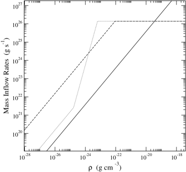
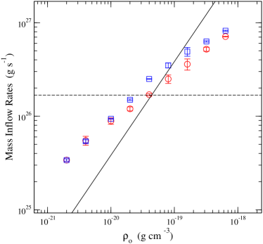
Figure 1: Left panel: The mass-accretion rates from various models: the Bondi accretion model (Bondi 1952) (solid), the modified Bondi accretion model by SDH05 (dashed) and that by BS09 (dotted), as described in Eqs. (2), (9) and (10), respectively. The mass-accretion rates are computed as a function of $\rho$ at a radius $r_{\mathrm{o}}$ which is much larger than $r_{\mathrm{B}}$, i.e., $r_{\mathrm{o}}\gg r_{\mathrm{B}}$. In all models, the speed of sound $c_{\mathrm{s}}$ at $r_{\mathrm{o}}$ is set to $520\,\mathrm{km\,s^{-2}}$, The mass of the BH is set to $M_{\mathrm{BH}}=10^{8}\,\mathrm{M_{\odot}}$. While $\alpha=100$ is adopted in the model of SDH05, $\beta=2.0$ is adopted in the model of BS09. In the modified Bondi accretion models of SDH05 and BS09, the mass-accretion rates are limited to the Eddington rate (Eq. [11]). Right panel: Comparison of the mass-inflow rates found in the HD simulations with those predicted by the Bondi accretion model (Bondi 1952) (solid line) and with those adopted by SDH05 and BS09 (dashed line). In the density range of the models considered here, $\dot{M}_{\mathrm{a}}$ adopted by SDH05 and BS09 are limited by the Eddington rate (Eq. [11]); hence, the line is flat. The mass-inflow rates at the inner boundary (circles) and those at the outer boundary (squares) of the computational domain are shown as a function of the outer boundary density $\rho_{\mathrm{o}}$. The simulations predict $\dot{M}_{\mathrm{a}}$ that are very similar to the Bondi accretion rates, but the models have a less steeper dependency on the density. The Bondi mass-accretions rates and those of SDH05 and BS09 are computed for the gas with the Comptonized temperature $T=2\times 10^{7}$ K and with $\gamma=5/3$. The figure is from Kurosawa et al. (2009).

2.2 AGN Feedback Models

Once $\dot{M}_{\mathrm{a}}$ is evaluated, one can estimate the amount of the accretion power that is released and deposited. In SDH05 and BS09 (also in many others, cf. Table 2 in BS09), $\epsilon_{\mathrm{r}}=0.1$ (e.g., Shakura & Sunyaev 1973; see also Soltan 1982) is assumed, and kept constant. A higher value of $\epsilon_{\mathrm{r}}$ ($\sim 0.2$) can be achieved in an accretion model with a thin disk and a rapidly rotating BH (e.g., Thorne 1974). Recent observations suggest a wide range of $\epsilon_{\mathrm{r}}$: $0.07$ (Martínez-Sansigre & Taylor 2009), $0.30$–$0.35$ (Wang et al. 2006a). On the other hand, Cao & Li (2008) find $\epsilon_{\mathrm{r}}$ is relatively low ($\sim 0.08$) for $M_{\mathrm{BH}}<10^{8}\,\mathrm{M_{\odot}}$ and relatively high ($\gtrsim 0.18$) for $M_{\mathrm{BH}}\gtrsim 10^{9}\,\mathrm{M_{\odot}}$. The exact mechanism coupling the accretion luminosity of a BH and the surrounding gas is not well known. Therefore, SDH05 and BS09 simply assumed that $L_{\mathrm{a}}$ couples only thermally (and isotropically) to the surrounding. Using Eq. (1), the rate of energy deposition to the surrounding (the AGN feedback rate) in SDH05 is

$$\dot{E}_{\mathrm{f}}=\epsilon_{\mathrm{f}}\,L_{\mathrm{a}}=\epsilon_{\mathrm{f}}\epsilon_{\mathrm{r}}\dot{M}_{\mathrm{BH}}c^{2}$$ (12)

where $\epsilon_{\mathrm{f}}$ is the efficiency of the AGN energy deposition to the surrounding gas, and is a free parameter which is to be constrained by observations. BS09 find the models with $\epsilon_{\mathrm{f}}=0.15$ matches observations (e.g., the Magorrian relation and the $M_{\mathrm{BH}}-\sigma$ relations) very well, and similarly SDH05 find $\epsilon_{\mathrm{f}}=0.05$ matches observations well.

3 Results from Our Numerical Simulations

In Kurosawa et al. (2009), we used our physical two-dimensional (2-D) and time-dependent hydrodynamical (HD) simulations of AGN flows to investigate the dependency of the BH mass-accretion rate on the surrounding gas density, and to measure the AGN feedback efficiencies in converting the accretion luminosity into the outward fluxes of energy, momentum and mass. To do this, we simply analyzed the simulations previously published in KP09. We note that 2-D simulations are consistent in many respects with their three-dimensional (3-D) counterparts (Kurosawa & Proga, 2009a).

3.1 Mass-Accretion Rates

The mass-inflow rates at the inner boundary $\dot{M}_{\mathrm{in}}\left(r_{\mathrm{i}}\right)$ and those at outer boundary $\dot{M}_{\mathrm{in}}\left(r_{\mathrm{o}}\right)$ from the HD simulations are plotted as a function of the outer boundary density $\rho_{\mathrm{o}}$ in the right panel of Fig. 1. For a given value of $\rho_{\mathrm{o}}$, $\dot{M}_{\mathrm{in}}\left(r_{\mathrm{i}}\right)$ and $\dot{M}_{\mathrm{in}}\left(r_{\mathrm{o}}\right)$ are not equal to each other, but rather $\dot{M}_{\mathrm{in}}\left(r_{\mathrm{i}}\right)<\dot{M}_{\mathrm{in}}\left(r_{\mathrm{o}}\right)$ because of an outflow. The lowest density model is an exception since no outflow is formed in this model. For the higher density models, an outflow forms, and not all the material entering from the outer boundary reaches the inner boundary. A fraction of gas experiences a strong radiation pressure and radiative heating, and the direction of flow changes, forming an outflow.

The figure also shows $\dot{M}_{\mathrm{a}}$ predicted by the Bondi accretion model (Eq. [2]) and those computed from the formulations of SDH05 and BS09 (Eqs. [9] and [10]). The outer radius is much smaller than that of a typical smoothing scale on a SPH cosmological simulation ($\sim 10^{3}$ pc), and the outer density values used in our simulations are much larger than a typical local density at BH in the SPH simulations. The higher density at a 10 pc scale is required to produce an outflow. For example, $\rho_{\mathrm{o}}$ must be greater than $2\times 10^{-21}\,\mathrm{g\,cm^{-3}}$, to form an outflow with our system setup. In the density range of the models considered here, $\dot{M}_{\mathrm{a}}$ adopted by SDH05 and BS09 are limited by the Eddington rate (Eq. [11]); hence, the line is flat (cf. left panel of Fig. 1).

We do not expect our solutions to reproduce the Bondi density dependency of the mass-inflow rate because they include the effects of radiative heating and radiation force. However, the right panel of Fig. 1 shows the mass-inflow rates from our models are very similar to those of the Bondi rates, i.e., the rates are of the same order of magnitude. Interestingly our $\dot{M}_{\mathrm{in}}\left(r_{\mathrm{i}}\right)$ and the Bondi mass-accretion rate matches around $\rho_{\mathrm{o}}=4\times 10^{-20}\,\mathrm{g\,cm^{-3}}$ which coincidentally corresponds to $\Gamma\approx 1$. The accretion rates from SDH05 and BS09 are Eddington (the rates corresponding to $\Gamma=1$) in this density range. Therefore their corresponding lines also cross at the same point.

Fig. 1 (right panel) shows that our models have a weaker dependency of the mass-inflow rates on the density than that of the Bondi accretion. The power-law fits of data points give the slope $q=0.52\left(\pm 0.01\right)$ for $\dot{M}_{\mathrm{in}}\left(r_{\mathrm{i}}\right)$ and $q=0.56\left(\pm 0.02\right)$ for $\dot{M}_{\mathrm{in}}\left(r_{\mathrm{o}}\right)$, which are indeed much smaller than that of the Bondi accretion model, i.e., $q=1$ (cf. Eq. [2]).

3.2 Feedback Efficiencies

Let us now consider AGN feedback efficiencies in energy, momentum and mass using the simulation results, as defined in Eqs. (4)–(6). The models used here show some degree of variability (typically $\sim 10\%$ level). Therefore, the physical quantities used to compute the feedback efficiencies are based on the time averaged values.

3.2.1 Energy Feedback Efficiency

Fig. 2 (left panel) shows the energy feedback efficiencies, $\epsilon_{\mathrm{t}}$, $\epsilon_{\mathrm{k}}$ and $\epsilon_{\mathrm{th}}$ computed based on our models, as a function of the Eddington ratio ($\Gamma$). For systems with relatively low Eddington ratio ($\Gamma$$\lesssim 0.4$), $\epsilon_{\mathrm{th}}>\epsilon_{\mathrm{k}}$. On the other hand, for systems with relatively high Eddington ratio ($\Gamma$$\gtrsim 0.6$), the kinetic feedback dominates the thermal feedback by a factor of $\sim 10$ to $\sim 100$. The model with $\Gamma=0.2$ does not form an outflow, indicating an approximate $\Gamma$ value below which no outflow forms (with our system setup).

The energy feedback efficiencies increase as $\Gamma$ increases, but the efficiencies saturate for $\Gamma\gtrsim 1$. The total energy feedback efficiency peaks at $\Gamma\approx 1$ with $\epsilon_{\mathrm{t}}\sim 10^{-4}$. The flattening of the efficiencies for $\Gamma\gtrsim 1$ is caused by the transition of the inflow-outflow morphology to a “disk wind” like configuration for the higher $\Gamma$ models (see fig. 4 in KP09). Because of the mismatch between the direction in which most of the radiation escapes (in polar direction) and the direction in which the most of the accretion occurs in the system (the equatorial direction), the radiatively driven outflows in the disk-wind-like configuration cannot increase the outflow efficiency by increasing the accretion luminosity or equivalently $\Gamma$. A similar behavior is found in the $\dot{M}_{\mathrm{out}}\left(r_{\mathrm{o}}\right)$– $\Gamma$ relation of KP09.

3.2.2 Mass Feedback Efficiency

Figure 2 (right panel) shows $\epsilon_{\mathrm{m}}$ plotted as a function $\Gamma$. The dependency of $\epsilon_{\mathrm{m}}$ on $\Gamma$ is very similar to that of the momentum feedback efficiency (not shown here). For $\Gamma\lesssim 1$, the mass feedback efficiency $\epsilon_{\mathrm{m}}$ increases as $\Gamma$ increases, but it starts to decreases slightly beyond $\Gamma\approx 1$. The efficiency peaks around $\Gamma=1$ with the maximum efficiency value $\sim 0.4$. In other words, about $40\%$ of the total inflowing mass is redirected to an outflow. The turn-around of $\epsilon_{\mathrm{m}}$ values is caused by the transition of the outflow morphology to a disk-wind-like configuration (see fig. 4 in KP09) for the larger $\Gamma$ models, as in the cases for the energy and momentum feedback efficiencies (Sec. 3.2.1).

The accretion process in our model is fundamentally different from that of the Bondi accretion model and those adopted in the cosmological simulations (e.g., SDH05; BS09) because in our model an outflow and an inflow can simultaneously be formed while the Bondi accretion model can only form an inflow. The model of SDH05 and others can form either an inflow or an accretion (but not both simultaneously).

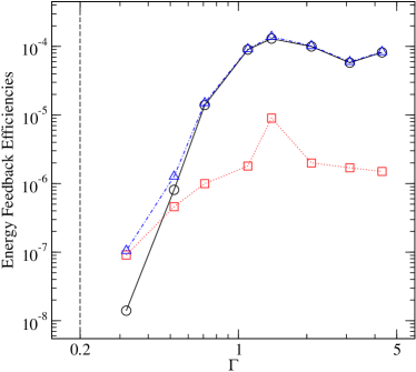
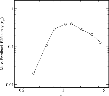
Figure 2: Left panel: the efficiencies of converting the BH accretion luminosity $L_{\mathrm{a}}$ to the rate of energy deposition to the surrounding gas are plotted as a function of the Eddington ratio ($\Gamma$). The panel shows the kinetic energy feedback efficiency $\epsilon_{\mathrm{k}}$ (circles), the thermal energy feedback efficiency $\epsilon_{\mathrm{th}}$ (squares) and the total energy feedback efficiency $\epsilon_{\mathrm{t}}=\epsilon_{\mathrm{k}}+\epsilon_{\mathrm{th}}$ (triangles), separately (see Eqs. [6], [7], and [8]). The maximum total energy feedback efficiency is $\sim 10^{-4}$. For the models with relatively low Eddington ratio ($\Gamma$$\lesssim 0.4$), the thermal feedback is more efficient than the kinetic feedback ($\epsilon_{\mathrm{th}}>\epsilon_{\mathrm{k}}$). For the models with relatively high Eddington ratio ($\Gamma\gtrsim 0.6$), the kinetic feedback is more efficient than the thermal feedback by a factor of $\sim 10$ to $\sim 100$. The model with $\Gamma=0.2$ does not form an outflow, and the vertical line (dashed) at $\Gamma=0.2$ indicates an approximate $\Gamma$ value below which no outflow forms. The flattening of the efficiencies at $\Gamma\approx 1$ is caused by the transition of the inflow-outflow morphology to a “disk wind” like configuration for the larger $\Gamma$ models (see fig. 4 in KP09). Right panel: the mass feedback efficiency ($\epsilon_{\mathrm{m}}$) plotted as a function the Eddington ratio ($\Gamma$). The efficiency peaks around $\Gamma=1$ with the maximum efficiency value $\sim 0.4$, i.e., $40\%$ of the total inflowing mass is converted to the outflows. The turn-around of $\epsilon_{\mathrm{m}}$ values is caused by the transition of the outflow morphology to a “disk wind” like configuration for the larger $\Gamma$ models (cf. KP09). The model with $\Gamma=0.2$ does not form an outflow, and the vertical line (dashed) at $\Gamma=0.2$ indicates an approximate $\Gamma$ value below which no outflow forms. The figures are from Kurosawa et al. (2009).

4 Conclusions

We performed over thirty number of axisymmetric, time-dependent radiation-hydrodynamical simulations of outflows from a slowly rotating (sub-Keplerian) infalling gas driven by the energy and pressure of the radiation emitted by the AGN (KP09). These simulations follow dynamics of gas under the influence of the gravity of the central $10^{8}~{}\mathrm{M_{\odot}}$ black hole on scales from $\sim 0.01$ to $\sim 10$ pc. They self-consistently couple the accretion-luminosity with the mass inflow rate at the smallest radius (a proxy for $\dot{M}_{\mathrm{a}}$). A key feature of the simulations is that the radiation field and consequently the gas dynamics are axisymmetric, but not spherically symmetric. Therefore, the gas inflow and outflow can occur at the same time.

The relatively large number of simulations allows us to investigate how the results depend on the gas density at the outer radius, $\rho_{\mathrm{o}}$. In a follow-up paper, Kurosawa et al. (2009), we measure and analyze the energy, momentum, and mass feedback efficiencies of the outflows studied in KP09. We compared our $\dot{M}_{\mathrm{a}}$-$\rho_{\mathrm{o}}$ relation with that predicted by the Bondi accretion model. For high luminosities comparable to the Eddington limit, the power-law fit ($\dot{M}_{\mathrm{a}}\propto\rho_{\mathrm{o}}^{q}$) to our models yields $q\approx 0.5$ instead of $q=1.0$ which is predicted by the Bondi model. This difference is caused by the outflows which are important for the overall mass budget at high luminosities. The maximum momentum and mass feedback efficiencies found in our models are $\sim 10^{-2}$ and $\sim 10^{-1}$, respectively. However, the outflows are much less important energetically: the thermal and kinetic powers in units of the radiative luminosity are $\sim 10^{-5}$ and $\sim 10^{-4}$, respectively. In addition, the efficiencies do not increase monotonically with the accretion luminosity, but rather peak around the Eddington limit beyond which a steady state disk-wind-like solution exists. Our energy feedback efficiencies are significantly lower than 0.05, which is required in some cosmological and galaxy merger simulations. The low feedback efficiencies found in our simulations could have significant implications on the mass growth of super massive black holes in the early universe.

References

- Begelman & Nath (2005) Begelman, M. C. & Nath, B. B. 2005, MNRAS, 361, 1387
- Bondi (1952) Bondi, H. 1952, MNRAS, 112, 195
- Booth & Schaye (2009) Booth, C. M. & Schaye, J. 2009, arXiv:0904.2572 (BS09)
- Cao & Li (2008) Cao, X. & Li, F. 2008, MNRAS, 390, 561
- Ciotti & Ostriker (1997) Ciotti, L. & Ostriker, J. P. 1997, ApJ, 487, L105
- Ciotti et al. (2009) Ciotti, L., Ostriker, J. P., & Proga, D. 2009, ApJ, 699, 89
- Di Matteo et al. (2005) Di Matteo, T., Springel, V., & Hernquist, L. 2005, Nature, 433, 604
- Fabian et al. (2006) Fabian, A. C., Celotti, A., & Erlund, M. C. 2006, MNRAS, 373, L16
- Ferrarese & Merritt (2000) Ferrarese, L. & Merritt, D. 2000, ApJ, 539, L9
- Gebhardt (et al. 2000) Gebhardt, K. et al. 2000, ApJ, 539, L13
- Hopkins et al. (2005) Hopkins, P. F., et al. 2005, ApJ, 630, 705
- Kurosawa & Proga (2008) Kurosawa, R. & Proga, D. 2008, ApJ, 674, 97
- Kurosawa & Proga (2009a) Kurosawa, R. & Proga, D. 2009a, ApJ, 693, 1929
- Kurosawa & Proga (2009b) Kurosawa, R. & Proga, D. 2009b, MNRAS, 397, 1791
- Kurosawa et al. (2009) Kurosawa, R., Proga, D., & Nagamine, K. 2009, ApJ, 707, 823
- Martínez-Sansigre & Taylor (2009) Martínez-Sansigre, A. & Taylor, A. M. 2009, ApJ, 692, 964
- Merloni & Heinz (2008) Merloni, A. & Heinz, S. 2008, MNRAS, 388, 1011
- Proga (2007) Proga, D. 2007, ApJ, 661, 693
- Proga et al. (2008) Proga, D., Ostriker, J. P., & Kurosawa, R. 2008, ApJ, 676, 101
- Sazonov et al. (2005) Sazonov, S. Y., Ostriker, J. P., Ciotti, L., & Sunyaev, R. A. 2005, MNRAS, 358, 168
- Schaye (2004) Schaye, J. 2004, ApJ, 609, 667
- Shakura & Sunyaev (1973) Shakura, N. I. & Sunyaev, R. A. 1973, A&A, 24, 337
- Sijacki et al. (2007) Sijacki, D., Springel, V., di Matteo, T., & Hernquist, L. 2007, MNRAS, 380, 877
- Soltan (1982) Soltan, A. 1982, MNRAS, 200, 115
- Springel et al. (2005) Springel, V., Di Matteo, T., & Hernquist, L. 2005, MNRAS, 361, 776 (SDH05)
- Thorne (1974) Thorne, K. S. 1974, ApJ, 191, 507
- Tremaine (et al. 2002) Tremaine, S. et al. 2002, ApJ, 574, 740
- Wang et al. (2006a) Wang, J.-M., Chen, Y.-M., Ho, L. C., & McLure, R. J. 2006, ApJ, 642, L111