Collective oscillations in disordered neural networks

Abstract

We investigate the onset of collective oscillations in a network of pulse-coupled leaky-integrate-and-fire neurons in the presence of quenched and annealed disorder. We find that the disorder induces a weak form of chaos that is analogous to that arising in the Kuramoto model for a finite number $N$ of oscillators [O.V. Popovich at al., Phys. Rev. E 71 065201(R) (2005)]. In fact, the maximum Lyapunov exponent turns out to scale to zero for $N\to\infty$, with an exponent that is different for the two types of disorder. In the thermodynamic limit, the random-network dynamics reduces to that of a fully homogenous system with a suitably scaled coupling strength. Moreover, we show that the Lyapunov spectrum of the periodically collective state scales to zero as $1/N^{2}$, analogously to the scaling found for the ‘splay state’.

I Introduction

One of the most general and relevant dynamical phenomena observed in the mammalian brain is the rythmic coherent behaviour involving different neuronal populations buszaki . The dynamics of neural circuits has been widely studied, by invoking various kinds of neuron models; collective oscillations are commonly associated with the inhibitory role of interneurons interneurons . However, coherent activity patterns have been observed also in “in vivo” measurements of the developing rodent neocortex and hyppocampus for a short period after birth allene , despite the fact that at this early stage the nature of the involved synapses is essentially excitatory review .

Independently, theoretical studies of fully coupled excitatory networks of leaky integrate-and-fire (LIF) neurons have revealed the onset of macroscopic collective periodic oscillations vvres ; mohanty (CPOs). This dynamical state is quite peculiar: the collective oscillations are a manifestation of a partial synchronization among the neuron dynamics and this is one way of identifying this phenomenon, which is, however, more subtle: the macroscopic period of the oscillations does not coincide with (is longer than) the average interspike-interval ISI of the single neurons and the two quantities are irrationally related. In fact, this phenomenon is also called self-organized quasi periodicity and can be observed in a wide class of globally coupled systems piko . In the context of pulse-coupled neural networks, CPOs arise from the destabilization of a regime characterized by a constant mean-field and a strictly periodic evolution of the single neurons: this regime, termed “splay state”, has been widely studied in several contexts, including computational neuroscience abbott .

Since real neural circuits are not expected to have a full connectivity koch , it is important to investigate the role of dilution on the occurrence of the stability of CPO. We do so by investigating an excitatory network of LIF neurons with 20% of missing links in two different setups: quenched disorder, where the network topology is fixed; annealed disorder, where the active connections are randomly and independently chosen at each pulse emission. As a first step, we rewrite the dynamical equations as a suitable event driven map, by extending the approach developed in zillmer2 . We do so by introducing a pair of variables for each neuron, to account for the evolution of the local electric field. This step is particularly important for the computation of the Lyapunov exponents, as it allows expressing the evolution equations into a “canonical” form and thereby simplifies the implementation of standard dynamical-system tools.

We find that the regime of CPOs is robust against the presence of dilution, both in the quenched and annealed setup. However, at variance with the homogeneous fully-coupled case, the dynamics of finite disordered networks turns out to be chaotic, although the degree of chaoticity decreases with the number $N$ of neurons. In fact, the maximum Lyapunov exponent goes to zero as $1/N^{\beta}$. The exponent $\beta$ is smaller in the quenched setup, indicating that finite-size effects are stronger. In the homogeneous case, we are able to determine the full Lyapunov spectrum for sufficiently large numbers of neurons. As a result, we find that the first band of the spectrum scales as that of the splay state abbott ; calamai , namely as $1/N^{2}$

The paper is organized as follows. In section II we introduce the model and the event-driven map that is used to carry out the stability analysis. In Sec. III we discuss the collective dynamical behaviours observed in the presence of disorder. Sec. IV is devoted to the Lyapunov analysis of these coherent solutions in the large $N$ limit. Finally, in Sec. V, we summarize the main results and the open problems.

II The model

We study a network of $N$ neurons, whose individual dynamics is modelled as a LIF oscillator. Following Refs. zillmer2 , the membrane potential $x_{i}(t)$ of the $i-th$ oscillator evolves according to the differential equation

$$\dot{x}_{i}(t)=a-x_{i}(t)+g\,E_{i}(t)\,\quad\quad i=1,\cdots,N\\$$ (1)

where $a>1$ is the suprathreshold input current and $g>0$ gauges the coupling strength of the excitatory interaction with the neural field $E_{i}(t)$. At variance with the fully-coupled network, where all neurons depend on the same “mean field” $E(t)$, here we consider a general setup, where neurons have different connectivities inside the network. As a result, it is necessary and sufficient to introduce an explicit dependence of the neural field on the index $i$. The discharge mechanism operating in real neurons is modelled by assuming that when the membrane potential reaches the threshold value $x_{i}=1$, it is reset to the value $x_{i}=0$, while a pulse is transmitted to and instantaneously received by the connected neurons. The field $E_{i}(t)$ is represented as the linear superposition of the pulses received by neuron $i$ at all times $t_{n}<t$: the integer index $n$ orders the sequence of the received pulses. Each pulse is weighted according to the strength of the connection $C_{j,i}$ between the emitting ($j(n)$) and the receiving ($i$) neuron. In general, the connectivity matrix $\bf C$ is assumed to be non-symmetric. In formulae,

$$E_{i}(t)=\frac{\alpha^{2}}{N}\sum_{n|t_{n}<t}C_{j(n),i}(t-t_{n})\theta\bigg{(}t-t_{n}^{(i)}\bigg{)}\exp\left[-\alpha(t-t_{n})\right]$$ (2)

where $\theta(x)$ is the Heavyside function and $\alpha$ is the inverse pulsewidth (the pulse shape has been chosen as in Ref. vvres ; abbott ) . Since also in the diluted case we will consider massively connected networks hansel , where the average number of synaptic inputs per neuron varies proportionally to the system size, it is natural to scale the synaptic strength with $N$ as done in Eq. (2).

The model is fully characterized by the two sets of equations (1) and (2). The dynamical system has a peculiar mathematical structure, with the field variable appearing as a memory kernel, which involves a summation over all past spiking events. We find much more convenient to turn the explicit equation (2) into the implicit differential equation

$$\ddot{E}_{i}(t)+2\alpha\dot{E}_{i}(t)+\alpha^{2}E_{i}(t)=\frac{\alpha^{2}}{N}\sum_{n|t_{n}<t}C_{j(n),i}\delta(t-t_{n})\ .$$ (3)

As a result, the dynamics of the neural network model takes the more “canonical” form of a set of coupled ordinary differential equations (1,3), which can be analyzed with the standard methods of dynamical systems (see e.g., vvres ; abbott ; zillmer2 ; calamai ) .

II.1 Event-driven map

The presence of $\delta$-like pulses into the set of coupled differential equations (1) and (3) may still appear as an intrinsic technical difficulty for the estimation of the stability properties. Actually, the standard algorithms for the evaluation of Lyapunov exponents rely upon the integration of differentiable operators acting in tangent space (see benettin ). However, one can easily get rid of this problem by tansforming the differential equations into a discrete time event-driven mapping. This task can be accomplished by integrating Eq. (3) from time $t_{n}$ to time $t_{n+1}$ ($t_{n}$ representing the time immediately after the emission of the $n$-th pulse). An explicit mapping can be written by introducing the auxiliary variable $Q_{i}:=\alpha E_{i}+\dot{E}_{i}$,

$$E_{i}(n+1)=E_{i}(n){\rm e}^{-\alpha\tau(n)}+Q_{i}(n)\tau(n){\rm e}^{-\alpha\tau(n)}$$ (4a)

$$Q_{i}(n+1)=Q_{i}(n)e^{-\alpha\tau(n)}+C_{j(n+1),i}\frac{\alpha^{2}}{N}$$ (4b)

$$x_{i}(n+1)=x_{i}(n)e^{-\tau(n)}+a(1-e^{-\tau(n)})+gH_{i}(n)\,.$$ (4c)

Here $\tau(n)=t_{n+1}-t_{n}$ is the interspike time interval: it is determined by the largest membrane potential (identified by the label $m(n)$) reaching the threshold value $x_{m}=1$ at time $t_{n+1}$,

$$\tau(n)=\ln\left[\frac{a-x_{m}(n)}{a+gH_{m}(n)-1}\right]\ ,$$ (5)

where

$$H_{i}(n)=\frac{{\rm e}^{-\tau(n)}-e^{-\alpha\tau(n)}}{\alpha-1}\left(E_{i}(n)+\frac{Q_{i}(n)}{\alpha-1}\right)-\frac{\tau(n)e^{-\alpha\tau(n)}}{(\alpha-1)}Q_{i}(n)\,;$$ (6)

for the parameter values considered in this paper ($g>0$ and $a\leq 1$), $H_{i}(n)>0$.

Altogether, the model now reads as a discrete time map of $3N-1$ variables, $\{E_{i},Q_{i},x_{i}\}$: one degree of freedom, $x_{m(n)}=1$, is eliminated as a result of having constructed the discrete-time dynamics with reference to a suitable Poincaré-section. At variance with the usual approach (see e.g. Ref. coombes ), the evolution equation does neither involve $\delta$-like temporal discontinuities, nor formally infinite sequences of past events: the map is a piecewise smooth dynamical system.

For the sake of simplicity, we assume that the entries of the connectivity matrix $C_{j,i}$ are either 0 or 1 (the homogeneous fully-coupled case correspondingto $C_{j,i}=1$ for all $j$’s and $i$’s). If the entries are chosen randomly, symmetries are lost and the only way to determine the asymptotic state for a finite $N$ is by numerically simulating map (4). In what follows, we consider two different setups: the synaptic connections are randomly chosen and are constant in time (quenched disorder); each time a neuron fires, the neurons receiving the excitatory pulse are randomly chosen (annealed disorder).

II.2 Linear Stability Analysis

As usual, the stability of (4) can be analyzed by following the evolution of infinitesimal perturbations in the tangent space. The corresponding equations are obtained by linearizing (4) as follows,

$$\delta E_{i}(n+1)=e^{-\alpha\tau(n)}\delta E_{i}(n)+\tau(n)e^{-\alpha\tau(n)}\delta Q_{i}(n)-\left(\alpha E_{i}(n)(\alpha\tau(n)-1)Q_{i}(n)\right)e^{-\alpha\tau(n)}\delta\tau(n)\,,$$ (7a)

$$\delta Q_{i}(n+1)=e^{-\alpha\tau(n)}\left[\delta Q_{i}(n)-\alpha Q_{i}(n)\right]\delta\tau(n)\,,$$ (7b)

$$\delta x_{i}(n+1)=e^{-\tau(n)}[\delta x_{i}(n)-x_{i}(n)\delta\tau(n)]+ae^{-\tau}\delta\tau(n)+g\delta H_{i}(n)\quad i=1,\dots,N-1\quad;\quad\delta x_{m}(n+1)\equiv 0\,.$$ (7c)

An explicit expression of $\delta\tau(n)$ can be obtained by differentiating Eqs. (5,6)

$$\delta\tau(n)=\tau_{x}\delta x_{1}(n)+\tau_{E}\delta E(n)+\tau_{Q}\delta Q(n)\ ,$$ (8)

where $\tau_{x}:=\partial\tau/\partial x_{1}$ and analogous definitions are adopted for $\tau_{E}$ and $\tau_{Q}$. Moreover, $\delta H_{i}(n)$ is a short-cut notation for the linearizazion of expression (6), which in turn depends on $\delta E_{i}(n),\delta Q_{i}(n)$ and $\delta\tau(n)$. For more mathematical details see zillmer ; zillmer2 ; calamai .

The degree of chaoticity of a given dynamical state is obtained by computing the Lyapunov spectrum, i.e. the set of $3N-1$ exponential growth rates $\lambda_{i}$ along the independent directions in tangent space. The Lyapunov spectrum has been numerically estimated by implementing the standard algorithm benettin .

III Collective Dynamics

In the fully coupled homogeneous case the local fields $E_{i}$, $Q_{i}$ are independent of the index $i$ and the number of equations reduces to $N+1$. Depending whether $\alpha$ is smaller or larger than a critical value $\alpha_{c}(g)$, the dynamics either converges to a so-called splay state, with constant $E(t)$, or to a partially synchronized state, where $E(t)$ and $x_{i}(t)$ evolve periodically and quasi-periodically, respectively vvres ; mohanty .

This “mean-field” dynamics is expected to change in disordered networks. Given the neuron dependence of the fields $E_{i}$ and $Q_{i}$, we find it convenient to introduce the average variables,

$$\bar{E}(n)=\frac{1}{N}\sum_{k=1}^{N}E_{k}(n)\qquad;\qquad\bar{Q}(n)=\frac{1}{N}\sum_{k=1}^{N}Q_{k}(n)\ .$$ (9)

as a tool to characterize the resulting dynamical regimes and to compare with the homogeneous case. All the results reported in this paper have been obtained by fixing the fraction $f$ of missing connections equal to $f=0.2$. Numerical investigation for different choices of $f$ (not reported here) show similar results. In analogy with the analysis of the homogeneous case, we have chosen $\alpha$ as the main control parameter (one can easily realize that choosing $g$ would be equivalent).

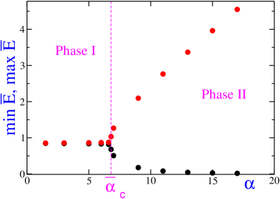
Figure 1: Minimal and maximal values of $\bar{E}(n)$ for different $\alpha$ values for $N=1,600$ with quenched disorder and $g=0.4$.

In Fig. 1 we plot the maximum and the minimum values of $\bar{E}(n)$ for different values of $\alpha$, for $g=0.4$ and $N=1600$ in the presence of quenched disorder. The bifurcation diagram is similar to the one observed in the globally coupled networks vvres . However, the splay state found for small $\alpha$-values has been replaced by a fluctuating asynchronous state, where the average field $\bar{E}(t)$ is only approximately constant (the difference between $\min\bar{E}(n)$ and $\max\bar{E}(n)$ is of the size of the symbols). The periodic collective state is analogously affected by small irregular fluctuations. This strong similarity between globally coupled and the diluted networks is not surprising: for any finite value of $f$, upon increasing $N$, the differences among the fields $E_{i}(t)$ should progressively disappear. In fact, in the limit $N\to\infty$, we expect randomly diluted networks to behave as fully coupled ones, provided that variables and parameters are properly rescaled. More precisely, the average field $\bar{E}(t)$ in a network with a fraction $f$ of missing links and a coupling constant $g$, is expected to be equivalent to the neural field $E$ generated in a fully coupled network with coupling constant $g(1-f)$. This expectation is confirmed by the critical value $\bar{\alpha}_{c}$ separating the two dynamical phases. As shown in Fig. 1, for $g=0.4$ and $f=0.2$, $\bar{\alpha}_{c}\sim 6.8$, a value which coincides, within the statistical error, with the critical value found in a globally coupled network with $g=0.32=0.4\times(1-0.2)$zillmer2 . A further consequence of the fact that the dynamics of disordered networks reduces in the thermodynamic limit to that of homogenous fully coupled ones is that the sample-to-sample fluctuations typical of quenched disorder should vanish as well. For this reason we have not performed averages of different realizations of the disorder.

A more detailed representation of the quenched dynamics above $\bar{\alpha}_{c}$ is obtained by looking at the projection in the plane $(\bar{E}(n),\bar{Q}(n))$. In Fig. 2 data sets are shown for $\alpha=9$ and increasing values of $N$: panels a and b correspond to the annealed and quenched case, respectively. This allows seeing that the two kinds of disorder yield indeed qualitatively similar results.

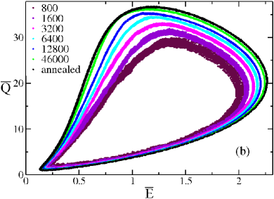
Figure 2: (Color online) $\bar{E}(n)$ versus $\bar{Q}(n)$ for various system syze: (a) annealed disorder and (b) quenched case here is shown also the annealed result for $N=100,000$. All data refers to $\alpha=9$.

More precisely, the phase points cluster around closed curves, revealing a “noisy” periodic dynamics. In the annealed case, the fluctuations can be attributed to the stochasticity of the evolution rule. Surprizingly, they are even larger in the quenched case, which correspond to a deterministic dynamics, in which case they must be attributed to the presence of deterministic chaos.

Upon increasing $N$, the amplitude of the fluctuations decreases and the attractor shape converges to an asymptotic curve, which should correspond to that of a homogeneous fully coupled network with a properly rescaled coupling strength $g$. This expectation is indeed confirmed in Fig. 3, where the attractor of a homogeneous network (with $N=1600$ and $g=0.32$) superposes to that of the annealed dynamics (with $N=10^{5}$ and $g=0.4$). In the quenched case, the asymptotic shape is the same, but the convergence is slower.

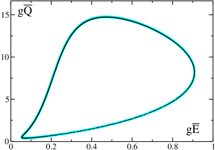
Figure 3: $g\bar{E}(n)$ versus $g\bar{Q}(n)$. The (blue) curve represents the attractor of a globally coupled system with $N=1,600$ and $g=0.32$, while the black dots refer to the annealed case with $N=100,000$ and $g=0.4$. For both cases $\alpha=9$ and $a=1.3$.

In order to investigate quantitatively the scaling behavior of the finite-size corrections, we have studied the $N$ dependence of

$$\Delta{\bar{Q}}=\langle{\bar{Q}}\rangle(N)-\langle{\bar{Q}}\rangle(\infty)$$ (10)

where the angular brackets denote the (time) average of $\bar{Q}$-value of all configurations falling within the lower $g\bar{E}(n)$-window [0.36, 0.44]. Since the asymptotic value $\langle{\bar{Q}}\rangle(\infty)$ is independent of the setup, we have extrapolated it in the simpler context of a fully coupled network with $g=0.32$ As a result, we find that $\Delta{\bar{Q}}$ always converges to zero as power-law, $N^{-\beta}$, with $\beta=1$ in the fully coupled network, $\beta=0.55$ for quenched disorder, and $\beta=0.82$ for annealed disorder (see Fig 4a). These latter values have to be considered as approximate estimates, affected both by statistical errors and finite-size corrections. A more accurate estimate is beyond our computational capabilities. However, for the present purpose, the relative differences are large enough to conclude that quenched disorder is characterized by a slower convergence.

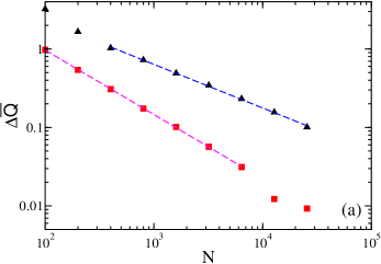
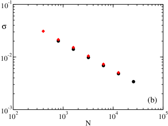
Figure 4: (Color online) (a) The quantity $\Delta\bar{Q}$ (see Eq. 10) versus the network size; (black) triangles refer to the quenched case, while (red) squares to the annealed one: data fits are reported as dashed lines. The reported values have been obtained by averaging over $6\times 10^{6}$ to $3\times 10^{7}$ consecutive spikes. (b) Standard deviation $\sigma$ (see Eq. 11) vs $N$ : circles and diamonds refer to the annealed and quenched case, respectively. The standard deviation have been averaged over $M=900$ iterates. All data refers to $f=0.2$, $\alpha=9$, $g=0.4$ and $a=1.3$.

As a further test of the collective dynamics, we have computed the standard deviation $\sigma(n)$ of the instantaneous fields

$$\sigma(n)=\left(\frac{\sum_{i=1}^{N}E_{i}^{2}({n})}{N}-\bar{E}^{2}({n})\right)^{1/2}\,,$$ (11)

which is a measure of the degree of synchronization among the various fields. In Fig. 4b we plot the time average $\langle\sigma\rangle$ for annealed and quenched disorder: in both cases $\langle\sigma\rangle$ decreases with $N$ as $N^{-1/2}$. These results confirm once more that in the limit $N\to\infty$ the neural field dynamics converges to that of homogeneous networks, irrespectively of the disorder.

IV Lyapunov analysis

In order to provide a more detailed characterization of the macroscopic as well as of the microscopic dynamics, in this section we analyse the Lyapunov spectra for the fully-coupled network and for its disordered variants.

IV.1 Globally Coupled Network

In this case, the fields seen by the neurons are equal to one another and it is therefore sufficient to introduce a single pair of field variables $E$ and $Q$. The corresponding stability analysis for the splay state has been analytically carried out in Ref. zillmer2 , finding that the spectrum of Floquet exponents is composed of a band of values of order $1/N^{2}$, which become of order ${\mathcal{O}}(1)$ at one band extremum, plus two isolated eigenvalues associated with the field dynamics. Therefore, it is convenient to start the numerical analysis by testing the effect of attaching a pair of field variables to each neuron. The results plotted in Fig. 5a refer to the Lyapunov spectrum of the splay state for $\alpha=3$ and $g=0.4$: one can observe two bands and two isolated exponents. The first band, composed of $N-1$ nearly vanishing exponents, and the two isolated exponents coincide with the eigenvalues analytically obtained in zillmer2 . The second band, composed of $2(N-1)$ exponents quantifies the transversal stability of the synchronization manifold $E_{i}=E_{1}$, $Q_{i}=Q_{1}$ $\quad\forall i$, where, without loss of generality, we consider the field of the 1st neuron as the reference variable. In fact, if one introduces the suitable difference variables,

$$w_{i}=E_{i}-E_{1}\qquad z_{i}=P_{i}-P_{1}\qquad i=2,\cdots,N\qquad.$$ (12)

the corresponding tangent dynamics is ruled by the equations

$$\delta w_{i}(n+1) = \delta w_{i}(n)e^{-\alpha\tau(n)}+\delta z_{i}(n)\tau(n)e^{-\alpha\tau(n)}$$ (13)

$$\delta z_{i}(n+1) = \delta z_{i}(n)e^{-\alpha\tau(n)}\qquad i=2,\cdots,N\quad.$$ (14)

This shows that the linearized dynamics of each pair of twin variables $(\delta w_{i},\delta z_{i})$ is decoupled from the rest of the network. Its stability can be evaluated by solving the corresponding two-dimensional eigenvalue problem. Accordingly, we expect two bands of $N-1$ eigenvalues each. However, since the two eigenvalues of Eq. (13) are both equal to $-\alpha$, we do have a single band, as indeed observed in Fig. 5a. As a last check, we have verified the $1/N^{2}$ scaling of the first band of the splay state. The nice overlap of the three sets of exponents corresponding to $N=100$, 200, and 400 with the analytical estimate calamai reported in Fig. 5c confirms the reliability of the numerical code.

The stability of CPOs arising when $\alpha>\alpha_{c}=8.34(1)$ vvres is not known. However, the above arguments concerning the presence of a single degenerate band still hold, as confirmed by the spectrum plotted in Fig. 5b, which corresponds to $g=0.4$, and $\alpha=9$. This adds to the first band that is again located just below zero, with the exception of the first exponent which is exactly equal to zero, as a result of the quasi-periodic dynamics of the single neurons (the second zero Lyapunov exponent has been discarded while taking the Poincaré section).

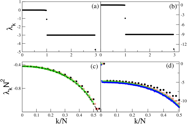
Figure 5: (Color online) Lyapunov exponents $\lambda_{k}$ versus $k/N$. Complete spectrum for $N=50$ for $\alpha=3$ (a) and $\alpha=9$ (b). Rescaled Lyapunov eigenvalues of the first band $\lambda_{k}\times N^{2}$ for different system sizes, namely $N=50$ (filled black circles), 100 (open red squares), 200 (green open triangles) and 400 (blue crosses), for $\alpha=3$ (c) and $\alpha=9$ (d). For $\alpha=3$ in (c) also the analytical expression (dashed black line) reported in Eq. (29) in calamai is shown. The data has been obtained by following the evolution in the tangent space of the event driven map for a number of consecutive spikes of the order of $10^{8}--10^{9}$, after discarding a transient composed by $50,000\times N$ spikes.

Finally, in Fig. 5d we have plotted the Lyapunov exponents of the first band multiplied by $N^{2}$. The tendency to overlap of the spectra obtained for $N=50,100,200,$ and 400 indicate that we are again in the presence of a $1/N^{2}$ scaling as for the splay states, although finite-size corrections are more relevant in this case. Accordingly, we conjecture that the $1/N^{2}$ dependence is a general property, which depends on the shape of the velocity field (see calamai ), rather than on the structure of the solution itself.

IV.2 Diluted Network

Since the collective solutions observed in the globally coupled network are characterized by many weakly stable directions, it is reasonable to expect that generic perturbations of the network dynamics yield a chaotic evolution. On the other hand, in the thermodynamic limit we expect the inhomegenities induced by a random dilution to vanish. In fact, we have already seen (in the previous section) that a macroscopically periodic dynamics is eventually recovered.

First of all we have verified that the network dynamics is chaotic for finite $N$, as soon as $f>0$. In Fig. 6a one can appreciate the growth of the maximal (positive) Lyapunov exponent with the fraction of missing links $f$ (in the quenched case).

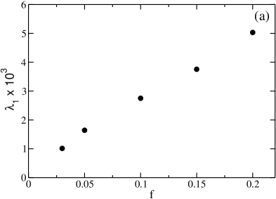
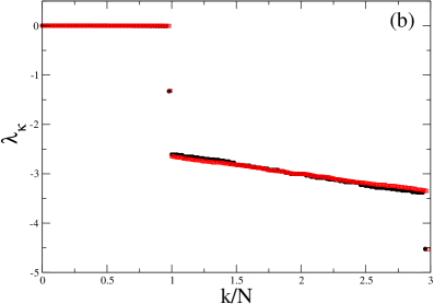
Figure 6: (a) Maximal Lyapunov exponent $\lambda_{1}$ as a function of the percentage $f$ of broken links for $N=800$ and $\alpha=9$. (b) Lyapunov spectrum $\{\lambda_{k}\}$ versus $k/N$ for $\alpha=3$ with networks of size $N=50$ (filled black circles) and $N=100$ (open red squares) and 20% of broken links. The data has been obtained by following the evolution of the event driven map and of the associated linearized equations ruling the evolution of the Lyapunov vectors for $3-4\times 10^{8}$ consecutive spikes, after discarding a transient composed by $300,000-600,000$ spikes. The data refers to quenched disorder.

For $\alpha=3$, analogously to the globally coupled case, the spectrum is composed of two bands and two isolated eigenvalues (see Fig. 6b). On the one hand, the degeneracy among the exponents lying in the second band is lifted (as a consequence of the disordered network structure) and the second band acquires a finite width. On the other hand, the comparison between the spectrum obtained for $N=50$ and $N=100$, reveals that the band width shrinks with $N$ around the value $\lambda=-\alpha$. This result again confirms that the inhomogenities of the disordered network vanish in the thermodynamic limit. A similar scenario occurs also in the CPO regime, as well as for annealed disorder.

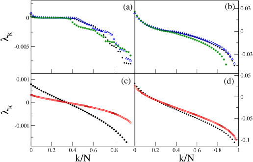
Figure 7: First band of the Lyapunov spectra $\{\lambda_{k}\}$ versus $k/N$ for $g=0.4$ with 20% of broken links for quenched disorder with $\alpha=3$ (a) and 9 (b) and for annealed disorder with $\alpha=3$ (c) and 9 (d). For the quenched disorder only spectra corresponding to system size $N=50$ are shown but for three different random network configurations, while in the annealed case spectra for network sizes $N=50$ (filled black circles) and $N=100$ (open red squares) are reported. The data has been obtained by following the evolution of the system and of its linearized copies for time lags similar to those reportd in the caption of Fig. 6.

Furthermore, in Fig. 7 (where we plot the first band of the Lyapunov spectrum for quenched and annealed disorder, in both dynamical phases), we see a variable number of positive exponents, indicating that finite disordered networks are typically chaotic. More precisely, panels $a$ and $b$ of Fig. 7, refer to quenched disorder. In both cases, we present the spectra resulting from three different realizations of the disorder. We see that sample-to-sample fluctuations are quite relevant in the second part of the band, while they affect less the largest exponents. Another qualitative observation concerns the shape of the spectrum that seems to be smoother in the presence of CPOs. Unfortunately, it is almost impossible to perform a quantitative scaling analysis of the spectrum (given the need to average over different realizations and to consider yet larger network sizes). In the annealed case, Fig. 7c/d, there is no need to average over different realizations of the disorder and the Lyapunov spectra turn out to be smooth. However a scaling analysis is still beyond our computer capabilities: in both cases we report the spectra obtained for $N=50$ and $N=100$ which are far from exhibiting a clean scaling behavior (for this reason we do not even dare to formulate a conjecture).

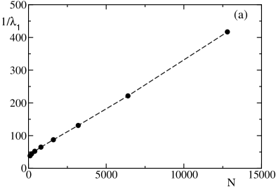
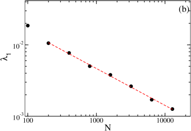
Figure 8: Maximal Lyapunov exponent $\lambda_{1}$ versus $N$: (a) annealed case; (b) quenched case. In the quenched case also a power-law fit is reported (red dashed line) with decay exponent $\beta=0.51\pm 0.01$. The data has been obtained by following the evolution in the tangent space of the event driven map for $10^{8}--10^{9}$ consecutive spikes, after discarding a transient of $200,000$ spikes. Both figures refer to 20 % of dilution, with parameters $\alpha=9$, $g=0.4$ and $a=1.3$.

Given the difficulties of dealing with the whole Lyapunov spectrum, we have concentrated our efforts on the maximum exponent $\lambda_{1}$, since we are thereby able to study larger networks. We limited ourselves to studying the CPO regime. As shown in Fig. 8, $\lambda_{1}$ decreases with $N$ as a power law: in the annealed case, $\lambda_{1}\approx 1/N$, while in the quenched case $\lambda_{1}\approx 1/\sqrt{N}$. This is at variance with the Kuramoto model, where in the “equivalent” quenched case, a $1/N$ behaviour has been observed maistrenko . Accordingly, although annealed networks are more chaotic than the quenched ones over the numerically accessible network sizes, we conclude that the opposite will be true for yet larger networks.

V Conclusions and perspectives

Our numerical analysis suggests that in the thermodynamic limit, a random, uncorrelated network behaves like a homogeneous globally coupled system with a rescaled value of the coupling constant to account for the different fraction of active links. This is because each neuron receives a random series of spikes: when the number of neurons increases, the number of spikes per unit time increases as well, while the relative fluctuations decrease and all neurons are affected by increasingly similar forcing fields (for a discussion on the thermodynamic limit in neural networks see also hansel ; vogels ). While there are little doubts that the collective motion is independent of the presence of disorder, less compelling is the evidence that the same is true for the stability properties. This is because numerical simulations are computationally expensive and it is not possible (at least for us) to study the scaling behavior of the entire Lyapunov spectrum in disordered systems. This is doable in homogeneous networks, thanks also to a faster convergence to the thermodynamic limit, and we have indeed observed that the first band of the Lyapunov spectrum scales as $1/N^{2}$, exactly as in the splay state, a case that is analytically known calamai . In disordered networks we have nevertheless been able to study the scaling behaviour of the maximal Lyapunov exponent, finding that it is positive and scales as $1/N^{\beta}$, with $\beta$ close to $1/2$ (resp. 1) in the quenched (resp. annealed) case. This means that deterministic chaos disappears in the thermodynamic limit. This observation is consistent with the fact that the collective motion is periodic: a periodically forced phase oscillator (such as a LIF neuron) cannot be chaotic. However, nothing seems to prevent the collective motion itself to be chaotic. Whether different connection topologies have to be invoked or yet unidentified constraints forbid this to occur, remains as an open question.

- (1) G. Buzsáki, Rhythms of the Brain (Oxford University Press, 2006)
- (2) M. A. Whittington and R. D. Traub, Trends in Neurosciences, 26 (2003) 676.
- (3) C. Allene, A. Cattani, J.B. Ackman, P. Bonifazi, L. Aniksztejn, Y. Ben-Ari, R. Cossart, The Journal of Neuroscience 26 12851-12863 (2008).
- (4) Y. Ben-Ari et al., Phisiol. Rev. 87 1215-1284 (2007)
- (5) C. van Vreeswijk, Phys. Rev. E 54, 5522 (1996).
- (6) P.K. Mohanty, A. Politi, J. Phys. A 39, L415 (2006).
- (7) M. Rosenblum and A. Pikovsky, Phys. Rev. Lett. 98, 064101 (2007).
- (8) L.F. Abbott and C. van Vreeswijk, Phys. Rev. E 48, 1483 (1993).
- (9) C. Koch, Biophysics of computation, Oxford University Press, New York (1999).
- (10) R. Zillmer, R. Livi, A. Politi, and A. Torcini, Phys. Rev. E 76 046102 (2007)
- (11) M. Calamai, A. Politi, and A. Torcini, Phys. Rev. E 80, 036209 (2009).
- (12) D. Golomb, D. Hansel, and G. Mato, (2001), “Theory of synchrony of neuronal activity” in Handbook of biological physics eds. S. Gielen and F. Moss (Amsterdam, Elsevier, 2001).
- (13) I. Shimada and T. Nagashima, Prog. Theor. Phys. 61, 1605 (1979); G. Benettin, L. Galgani, A. Giorgilli and J.M. Strelcyn, Meccanica, March 15 and 21 (1980).
- (14) S. Coombes, Proceedings of Stochastic and Chaotic Dynamics in the Lakes, AIP Conference Proceedings, 502, 88 (1999)
- (15) R. Zillmer, R. Livi, A. Politi, and A. Torcini, Phys. Rev. E 74 036203 (2006)
- (16) O.V. Popovich, Y.L. Maistrenko, and P.A. Tass, Phys. Rev. E 71 065201(R) (2005)
- (17) T.P. Vogels, K. Rajan, and L. F. Abbott, Annu. Rev. Neurosci. 28, 357 (2005).