Filamentation processes and dynamical excitation of light condensates in optical media with competing nonlinearities

Abstract

We analyze both theoretically and by means of numerical simulations the phenomena of filamentation and dynamical formation of self-guided nonlinear waves in media featuring competing cubic and quintic nonlinearities. We provide a theoretical description of recent experiments in terms of a linear stability analysis supported with simulations, showing the possibility of the observation of modulational instability suppression of intense light pulses travelling across such nonlinear media. We also show a novel mechanism of indirect excitation of light condensates by means of coalescence processes of nonlinear coherent structures produced by managed filamentation of high power laser beams.

I Introduction

Studies on nonlinear beam filamentation of ultrashort pulses are being actively developed nowadays filamentation1 . Far beyond a certain critical power threshold, extremely short pulses may become unstable and break up into several uncorrelated light structures by modulational instability (MI) processes. These structures, called filaments in this context, are spatiotemporal soliton-like light distributions which appear after MI and hold for large propagation distances without changing their shape and sizefilamentation2 . In fact, optical filaments have been observed in several scenarios like airfilamentation1 , waterdubietis03 , carbon disulfidecenturion05 , etc., and some mechanisms to control their spatial location have been recently proposedRohwetter08 .

On the other hand, the theoretical description of these localized modes is in general based on nonlinear Schrödinger equations (NLSE)piekara74 ; dimitrievski98 ; Ting06 . In the modeling of these kind of systems, nonlinear effects like two and three photon absorption, second order group-velocity dispersion, time-delayed nonlinear response, multiphoton ionization and plasma defocusingfilamentation3 are usually taken into account. Nevertheless, in order to favor the insight of dynamics in these systems, simpler models are employed when certain physical conditions are satisfied. To this end it is common to consider NLSE involving just local intensity-dependent nonlinear susceptibilities which are realfilamentation3 . As an example, the so-called cubic-quintic (CQ) nonlinearityquiroga97 has been used as a solvent approximation in modelling subpicosecond pulse propagation in nonlinear mediacenturion05 . In the latter reference, the dynamics of filament formation and evolution in carbon-disulfide cells is analyzed both experimentally and by numerical means. At this respect, extensive numerical work based on a conservative CQ model is successfully employed in the qualitative description of experimental achievements.

In addition “liquid light condensates”, i.e, robust solitonic distributions in CQ optical media with a “flat-top” transverse spatial envelope and intriguing surface tension properties were studied in michinel . Recently, it was shown that their dynamics follows the same equations governing the evolution of usual liquid dropletsnovoa_PRL . These results were obtained by both analytical and numerical methods, but they have not yet been confirmed by real experiments. The main difficulty, of course, is the search for a cubic-quintic nonlinear medium, although some candidates were inspected in smektala00 . In fact, both nonlinear third and fifth order terms in the polarization of the material are usually complex, so it is often necessary to consider some other nonlinear processes like ones related above. Nevertheless, in the light of Ref.centurion05 we are allowed to think of materials like $CS_{2}$ as real CQ nonlinear media in specific power regimes. Recently, some common gases like air, $N_{2}$ and $O_{2}$ have also been identified as CQ optical media by means of the measurement of $n_{4}$ coefficientscq_demo09 , although the propagation dynamics of probe pulses throughout these media has not yet been investigated.

The purpose of the present paper is threefold. Firstly, we will give a simple theoretical description of the results obtained in centurion05 by means of a linear stability analysis of plane waves. Secondly, we will study both analytically and numerically the possibility of real observation of the modulational instability suppression process in $CS_{2}$ . Finally, we will provide a detailed description of a novel mechanism of dynamical excitation of flat-top solitons in “pure” CQ systems via filamentation management and coalescence and we will analyze the possibility of achieving light condensates in carbon disulfide.

II Physical model

We will consider the propagation of a high-intensity laser pulse through a $CS_{2}$ bulk, within the framework of the nonlinear Schrödinger equation (NLSE). In order to simplify the theoretical model, we assume a scalar slowly varying spatial envelope and we neglect group-velocity dispersion effects. These approximations have been experimentally justified for media like carbon disulfidecenturion05 and airfilamentation3 within proper parameter spaces. We will also include a cubic-quintic nonlinearity, resulting in the following NLSE

$$2ik_{0}n_{0}\frac{\partial\psi}{\partial z}+\nabla_{\perp}^{2}\psi+2k_{0}^{2}n_{0}(n_{2}|\psi|^{2}-n_{4}|\psi|^{4})\psi=0$$ (1)

where the quantities above are defined as follows: $\psi$ is the complex slowly varying electric field envelope of the corresponding electromagnetic wave propagating through the nonlinear medium. $k_{0}=2\pi/\lambda$ is the vacuum wavenumber corresponding to the laser source wavelength $\lambda$. $n_{0}$ is the linear refractive index of the medium and $z$ is the propagation distance. Nonlinear coefficients $n_{2},n_{4}$ characterize the strength of the real third and fifth order nonlinear optical susceptibilities respectively. $\nabla^{2}_{\perp}=\partial^{2}/\partial{x^{2}}+\partial^{2}/\partial{y^{2}}$ is the Cartesian transverse Laplacian operator. Notice that Eq.1 preserves the norm of the field $\Psi$, i.e. we have also neglected the effect of nonlinear two-photon absorption, which can be justified for moderate intensity pulses travelling throughout a carbon disulfide bulk over a short distance centurion05 .

For technical reasons related with numerical treatment of partial differential equations, it is often useful to express Eq.(1) in a reduced form by introducing a suitable set of non-dimensional variables, namely

$$i\frac{\partial\Phi}{\partial\eta}+\Delta\Phi+(|\Phi|^{2}-|\Phi|^{4})\Phi=0$$ (2)

where the adimensional variables considered from now on are: $\eta=zk_{0}n_{2}^{2}/n_{4}$ is the adimensional propagation distance, $\Delta=\partial^{2}/\partial{\chi^{2}}+\partial^{2}/\partial{\zeta^{2}}$ is the dimensionless transverse Laplacian operator, being the spatial coordinates $\Theta=\theta k_{0}n_{2}\sqrt{2n_{0}/n_{4}}$, with $\Theta=\chi,\zeta$, $\theta=x,y$. The normalized beam irradiance $|\Phi|^{2}=(n_{4}/n_{2})|\psi|^{2}$ is measured in units of the quotient $n_{4}/n_{2}$ which univocally characterizes the nonlinear response of the medium.

Keeping in mind the equivalence between Eqs.1 and 2, typical parameters corresponding to beam propagation in real dielectric materials like $CS_{2}$ are (for femtosecond optical pulses with $\lambda=800nm$Ganeev04 ) $n_{0}=1.6$, $n_{2}=3\cdot 10^{-15}cm^{2}/W$. To our best knowledge, the $CS_{2}$ quintic coefficient $n_{4}$ has not been measured yet, since there are no values of this quantity cited in the literature, although an approximation $n_{4}=2\cdot 10^{-27}cm^{4}/W^{2}$ based on the agreement between simulations and experiments was successfully introduced in centurion05 . Very remarkably, the first experimental determination of the nonlinear coefficient $n_{4}$ of several gaseous media has been recently carried out in cq_demo09 .

In the following section, we will introduce an analytical linear stability analysis of plane waves in the CQ model and its results will be compared with those of the experiments in centurion05 .

III Linear stability analysis of plane waves

It is well known that Eq.2 admits plane wave (PW) solutions of the type $\Phi=\Phi_{0}e^{i\gamma\eta}$, where $\Phi_{0}$ is a constant which depends on $\gamma$ eigenvalues as follows:

$$\Phi_{0}=\Bigg{[}\frac{1}{2}+\frac{\sqrt{1-4\gamma}}{2}\Bigg{]}^{\frac{1}{2}}$$ (3)

Let us proceed with a linear stability analysis of these homogeneous solutions, following the Bespalov-Talanov procedurebespalov66 . The first step of this method is to add a small amplitude perturbation of the form $\xi=\xi_{R}+i\xi_{I}$ to the PW solutions, with $\xi_{R,I}=\xi_{R,I}^{0}e^{[i{\bf K_{\perp}}\cdot{\bf r}+ih\eta]}$ and $|\xi_{R,I}|\ll\Phi_{0}$, where ${\bf K_{\perp}}$ is the transverse wavevector and $h$ is the propagation constant of the corresponding perturbational mode. Now, for $h^{2}<0$, depending on the sign of $\Im(h)$, we have two possible outcomes. If $\Im(h)<0$, the perturbations grow exponentially in $\eta$ yielding to field destabilization. However, if $\Im(h)>0$ the amplitude of the perturbational mode decays quickly, so that the underlying PW remains stable. On the contrary, whenever $h^{2}>0$, the amplitude of the perturbations remains limited.

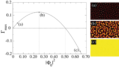
Figure 1: Plot of $\Gamma_{max}$ vs. $|\Phi_{0}|^{2}$. The highest growth rate corresponds to $\Phi_{0}^{2}=0.25$, whereas for $\Phi_{0}^{2}\geq 0.5$ all values $\Gamma_{max}$ vanish or become negative delimiting the domain of modulational instability suppression. The labeled points on the graph refer to the pseudocolor intensity plots on the right side of the picture. These plots display a small region [width=$500$, height=$300$] of perturbed PW of intensities $\Phi_{0}^{2}=0.045$ (a), $\Phi_{0}^{2}=0.25$ (b), $\Phi_{0}^{2}=0.64$ (c) at the propagation distance $\eta=125$. The filaments shown in (b) arise before those in (a), so that both coalescence and domain formation effects can be observed.

By substituting the expression for the perturbed PW $\Phi=(\Phi_{0}+\xi)e^{i\gamma\eta}$ in Eq.2 and separating both the real and imaginary parts of the outgoing relation, we obtain, after linearizing on $\xi_{R},\xi_{I}$, i.e. retaining only the first order terms in perturbation theory, the following couple of Schrödinger-type equations

$$\frac{\partial\xi_{I}}{\partial\eta}-\Delta\xi_{R}-(2\Phi_{0}^{2}-4\Phi_{0}^{4})\xi_{R}=0$$ (4a)

$$\frac{\partial\xi_{R}}{\partial\eta}+\Delta\xi_{I}=0$$ (4b)

where $\xi_{R,I}$ depend upon $K_{\perp}$ and $h$ in the way noted above. From Eq.4b we obtain $\xi_{R}=\frac{K_{\perp}^{2}}{ih}\xi_{I}$, and taking into account Eq.4a we deduce the algebraic relation

$$\Gamma=K_{\perp}[-K_{\perp}^{2}+2\Phi_{0}^{2}-4\Phi_{0}^{4}]^{\frac{1}{2}}$$ (5)

where $\Gamma$ is the growth rate of the perturbations, satisfying $\Gamma=ih$. Notice that all the information about the PW perturbational spectrum is contained in the amplitude $\Phi_{0}$. We can estimate the value of the transverse wavevector which gives the maximum growth rate by looking for the extremals of Eq. 5, i.e

$$\frac{\partial\Gamma}{\partial K_{\perp}}=0\rightarrow(K_{\perp}^{max})^{2}=\Phi_{0}^{2}-2\Phi_{0}^{4}=\Gamma_{max}$$ (6)

As a consequence, the PW of amplitude $\Phi_{0}=\frac{1}{2}$ features the highest perturbation growth rate (see Fig.1). This means that it will suffer destabilization in a shorter characteristic scale than any other homogeneous solutions of Eq. 2, if it is perturbed by a harmonic mode with $K_{\perp}=K_{\perp}^{max}$. These assertions are illustrated by Figs.1-2. In Fig.1 we have plotted the quantity $\Gamma_{max}$ as a function of the PW intensity. For $|\Phi_{0}|^{2}>0$, we get $\Gamma_{max}\leq 0$, corresponding with the modulationally stable PW branchphysicaD . The three pseudocolor intensity plots in the right column snapshots of Fig.1 display different examples of the state of perturbed light homogeneous distributions after a propagation distance $\eta=125$. All PW considered throughout this manuscript are perturbed with a $5\%$ spatial random noise and propagated with a standard beam propagation method.

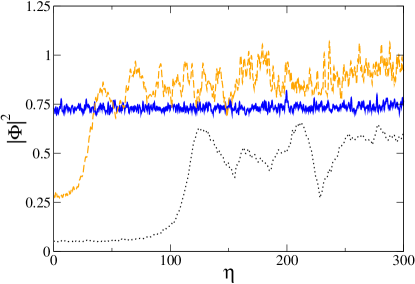
Figure 2: Plots of the peak intensity evolution over the line [$\zeta=0$,$-120<\chi<120$] of perturbed plane waves. Blue-solid line [$\Phi_{0}^{2}=0.64$] is almost constant, featuring small bounded oscillations due to spatial noise initially added. Orange-dashed line [$\Phi_{0}^{2}=0.25$] shows a rapid growing in intensity with $\eta$, which is a trace of a short longitudinal instability scale. Black-dotted line [$\Phi_{0}^{2}=0.045$] shows the destabilization scale for experimental datacenturion05 . It is important to notice the difference in between both instability scales of orange-black curves. For the simulation with experimental data, the starting point of the filamentation process is around $\eta=75$ ($2.1mm$ in dimensional units) which is compatible with that of experiments. In all cases, the maximum propagation distance is $\eta=300$.

The top picture Fig.1-(a) corresponds to a simulation with $\Phi_{0}^{2}=0.045$ (unstable PW). It is observed that this noisy distribution leads to the formation of several self-trapped optical channels which survive a long distance. We have chosen this intensity because it corresponds to one of those used in the experimentscenturion05 . We estimate the FWHM of the arising filaments to be around $10\mu m$, in good agreement with the experimental measurements. The middle picture Fig.1-(b) shows the last stage of a simulation with $\Phi_{0}^{2}=0.25$, corresponding to the PW with the highest $\Gamma_{max}$. In fact, as this PW posseses the shortest longitudinal scale of destabilization, it can be seen in Fig.1-(b) that after filament formation some domains are formed due to coalescence processes between self-guiding structures. The final example in the bottom picture Fig.1-(c) shows a stable PW of $\Phi_{0}^{2}=0.64$. This is a very interesting illustration of the phenomenon called modulational instability suppression (MIS). For $\Phi_{0}^{2}>0.5$, the linear perturbational modes decrease exponentially, thus leading to a suppression of the modulational instability which could be observed in real experiments. To our knowledge, this would constitute the first example of beam stabilization in a nonlinear optical medium obtained just by changing the input intensity.

Moreover, when the considered perturbations are intense enough, the quantity $\Gamma_{max}$ acquires a greater relevancy since its inverse value yields the characteristic longitudinal scale of instability development $\Lambda_{||}$bespalov66 . In a first approximation, we will consider the filamentation regime to be described by the coefficient $\Lambda_{||}$ as well as by the quantity $\Lambda_{\perp}=\pi/K_{\perp}^{max}$, which univocally characterizes the transverse spatial scale of the emerging filamentsbespalov66 ; filamentation3 . We are assuming throughout this paper that optical filaments are axially symmetric so that $\Lambda_{\perp}$ is valid for both transverse coordinates ($\chi,\zeta$). In general, both quantities ($\Lambda_{||}$, $\Lambda_{\perp}$) are useful in estimating the order of magnitude of different spatial instability scales, but their agreement with both simulations and experiments can be rather qualitative due to the existence of different filamentation regimes, radial perturbations, nonlinear responses, inhomogeneities in the medium, coalescence processes between filaments, etc. In any case, as multiple filamentation appears as a consequence of modulational instability of the corresponding field, the linear stability analysis should be at least qualitatively correct at the leading order, where other nonlinear processes are not considered to be involved.

In Fig.2, we have selected a transverse cut of the three paradigmatic PW considered above (see Fig.1) and we have determined their peak intensity along the propagation. As it can be appreciated, the perturbed PW with $\Phi_{0}^{2}=0.64$ (blue-solid line) features a quasi-constant intensity during the whole simulation, illustrating the MIS process. However, for $\Phi_{0}^{2}=0.25$ (orange-dashed) and $\Phi_{0}^{2}=0.045$ (black-dotted), a dramatic growing of the peak intensity with $\eta$ is observed, indicating the destabilization of the initial conditions. Furthermore, there is a substantial difference in the longitudinal instability scale of both situations. It can be appreciated that $\Phi_{0}^{2}=0.25$ (PW featuring the highest $\Gamma_{max}$) displays shorter instability scale than $\Phi_{0}^{2}=0.045$. Hereafter, we will compare this numerical result with the theory as well as the predictions of the stability analysis for the experimental parameters considered by Centurion et al. centurion05 , that observed the filamentation process undergone by femtosecond pulses propagating in $CS_{2}$. Using pulses of peak intensity $I_{p}=0.68$ $GW/mm^{2}$, they measured a mean filament sizes of $12\mu m$, in good agreement with our estimation. Moreover, the transverse scale of the filaments predicted by our linear stability analysis for their experimental configuration is $\Lambda_{\perp}=\pi/(\Phi_{0}^{2}-2\Phi_{0}^{4})^{\frac{1}{2}}$, or $\Lambda_{\perp}\approx 16.45\mu m$ in dimensional units, which is also consistent with the sizes measured in centurion05 . This can be interpreted as a further theoretical proof of the validity of the CQ model in describing the dynamics of femtosecond optical pulses propagating in $CS_{2}$.

On the other hand, the longitudinal scale of instability development $\Lambda_{||}$ can be estimated as $\Lambda_{||}\approx\Gamma_{max}^{-1}=24.4$ ($0.7mm$ in dimensional units). This scale has not been directly characterized by Centurion et al. in Ref. centurion05 . Nevertheless, they found completely developed filaments on a scale of $5mm$, which is compatible with our value of $\Lambda_{||}$, that constitutes a rough estimation of the propagation distance for the filaments when they start to grow up. Note that for $\Phi_{0}^{2}=0.25$ we get $\Lambda_{||}=8$, thus justifying the shorter characteristic scale of instability development observed in Fig.2.

While our analytical and numerical results for $\Lambda_{\perp}$ are both in good agreement with the experiment of Ref. centurion05 , the estimations for $\Lambda_{||}$ turn out to be less accurate. This is due to the fact that in the simulations we have perturbed the homogeneous distributions with random noise instead of using harmonic perturbations with fixed $K_{\perp}$. In fact, we have checked that using harmonic perturbations leads to smaller values for $\Lambda_{||}$ by a factor of $\sim 3$, getting closer to the analytical calculation.

These results show that, in spite of its simplicity, the linear stability analysis not only provides a good insight into the physics, but it can also be used to obtain quantitative useful predictions for the experiments of filamentation in $CS_{2}$.

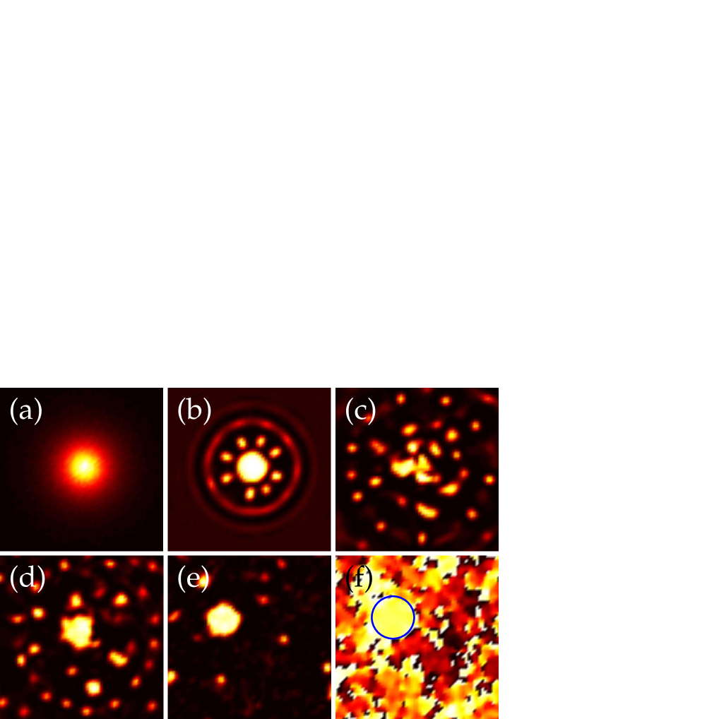
Figure 3: Intensity pseudocolor plots of the $SGF$ evolution in the presence of an unstable homogeneous background. The intensity snapshots correspond to a spatial domain [$-75<\chi,\zeta<75$] at several propagation distances, namely: (a) $\eta=0$; (b) $\eta=80$; (c) $\eta=150$; (d) $\eta=200$; (e) $\eta=1000$. Last picture (f) displays the phase map of the field depicted in (e). From this phase structure, it can be stated that the light condensate appearing at the last stage of the propagation is a coherent light structure since the color within the region where it is located (see blue circle in picture (f)) is homogeneous.

IV Liquid light solitons arising by coalescence

In this section we will show through numerical simulations a novel mechanism for the dynamical excitation of so-called “liquid light condensates”michinel in media with CQ nonlinearity, by means of spatial control of the filamentation regime and coalescence processes between self-guided optical channels. Furthermore, we will discuss about the possibility of observation of these structures in the experiments with $CS_{2}$.

As starting point, we have considered an initial condition for our simulations consisting on a broad-extended laser pulse with random noise fluctuations added. Group-velocity dispersion effects shall not be considered here since it is justified to assume that the temporal profile of the pulse does not change during short propagation distances through $CS_{2}$centurion05 . We will model this light distribution with a wide flat-top profile represented by the following function;

$$\Omega=A_{bg}\Big{[}0.25\Big{(}\Big{[}1+\tanh(\rho+\omega_{bg})\Big{]}\Big{[}1-\tanh(\rho-\omega_{bg})\Big{]}\Big{)}\Big{]}$$ (7)

where $A_{bg}$ is the peak amplitude of the light pulse, $\rho=\sqrt{\chi^{2}+\zeta^{2}}$ is the radial coordinate and $\omega_{bg}$ is the mean radius. We have performed all simulations fixing $A_{bg}=0.2$ and $\omega_{bg}=1000$. As we will restrict ourselves to a small region located at the center of the pulse, we can think of the domain delimited by $\Omega$ as part of a plane wave, since boundary effects (e.g. near-field diffraction) will not affect our results within the longitudinal scale imposed by the common experimental setups. We will explore the case $A_{bg}=0.2$, corresponding to a modulationally unstable plane wavephysicaD as we have discussed above, although the same qualitative behavior is obtained whenever $\Gamma_{max}>0$ (see Fig.1).

By adding an inhomogeneity to the light distribution of Eq. (7), we will be able to manage the filamentation regime. In fact, we have induced a small scale Gaussian fluctuation (SGF) of amplitude $A_{G}=0.5071$ and width $\omega_{G}=30$, located at the center of the bidimensional spatial profile $\Omega$ in order to select a small region where filamentation will first appear. Notice the scale difference between the two counterparts. Then by overlapping both structures $\Omega$ and $SGF$, we are generating a spatially inhomogeneous profile $\Phi_{in}$ with a peak intensity $|\Phi_{in}|^{2}=0.5$, which corresponds to that of the plane-wave defining the boundary between the stable and unstable PW solutions of Eq.1 physicaD .

The evolution dynamics of such light distribution is illustrated in Fig.3. In this figure, the snapshots show our small region of interest [$-75<\chi,\zeta<75$]. The initial condition is plotted in picture (a). Once the pulse has entered the medium, the $SGF$ starts to self-focus. It is remarkable how such a process is fastly counteracted by the self-defocusing nonlinearity. As a result, a bright hot spot is observed at the distribution centroid and diffractive rings representing shockwaves due to “background-fluctuation” interplay appear (see (b) snapshot).

The spectral properties of these waves (usually referred as conical emissions) have been studied in Nibbering96 . They give support to the formation of new filaments from pulse MI. Hereafter, we will discuss how to control the shockwave propagation in order to stimulate the appearance of several filaments surrounding the hot spot (see (b) snapshot). The key point is to generate a $SGF$ in a precise way by using phase masksRohwetter08 and techniques like pulse shaping pulse_shaping . To excite wide liquid solitons, we propose to surround the main custom-generated light structure, which is roughly similar to a top-flat beam, with a critical number of filaments located close of it. In fact, the solitons are statistical attractors due to their high internal energy. The satellite filaments are then used to provide an energy source for the central seed so that its power could be increased by coalescence processes, if the phases of the soliton and the filament match. As shown in snapshot (c) in Fig.3, there is indeed a dynamical energy exchange between filaments and hot spot during propagation. As a result, all solitonic structures are both created and annihilated several times (picture (c)), until a wider coherent structure with almost constant peak intensity arises (picture (d)). As a consequence, the emerging liquid light solitonmichinel is strongly perturbated by the energy excess released in the collective coalescence. Nevertheless, from snapshot (e) we see that after a large propagation distance the flat-topped soliton features an improved radial symmetry, the energy excess being radiated in the form of linear modes.

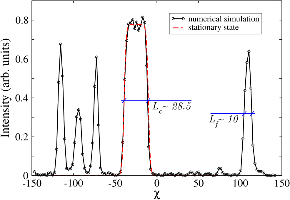
Figure 4: Transverse intensity profile of the filaments distribution (black solid line) at $\eta=5000$, with a superposed transverse profile of an eigenstate (red dashed line) of Eq. 2 with propagation constant $\gamma=0.173$. It is seen that the agreement between both contours is reasonable. $FWHM$ (delimited with blue solid lines) of the different-sized filaments represented in the figure have been estimated to be $L_{c}\approx 28.5$ (flat-topped soliton) and $L_{f}\approx 10$ (Kerr-type soliton). The spatial coordinate $\chi\in[-150,150]$.

In picture (f) we also show the phase map corresponding to the intensity plot displayed in (e). We see that within the region where the condensate is placed (highlighted with a blue circle) the phase structure is homogeneous.

Finally, we have checked the transverse size of the distribution after a huge propagation distance, $\eta=5000$. This allows the light condensate to relax towards a stationary state, thus minimizing random profile variations due to surface modes. In Fig.4, we have compared this extracted profile with that of a stationary solution of Eq.2. The agreement between the transverse profiles corresponding to this simulation and the stationary mode is remarkable. This completes the demonstration that this nonlinear structure observed in our simulations is a true flat-topped CQ-soliton.

To determine whether this kind of top-flatted transverse modes have been observed in the experiments with $CS_{2}$centurion05 , we have estimated their transverse size, and found that it would lie around the value $L_{c}\approx 28.5$ ($30.2\mu m$ in dimensional units). This is almost $3$ times greater than the size of the optical filaments measured in Ref. centurion05 . We thus conclude that Centurion et al. have not reached the threshold to produce top-flatted, liquid light solitons.

On the other hand, on the right side of the light condensate displayed in Fig.4 we also see a completely developed self-guided light channel of size $L_{f}\approx 10$ ($10.6\mu m$ in dimensional units), which resembles closely to those observed by Centurion et al.. This is a further demonstration that our simulations reasonably reproduce the existing observations, besides providing a guide for the new managed production of the higher power top-flatted solitons.

V Conclusions

In this paper, we have provided theoretical support to recent experiments on filamentation of ultrashort pulses propagating through carbon disulfide by means of approximate analytical methods and numerical simulations of propagation. The agreement between our calculations and the experimental outcomes is remarkable, taking into account that we have developed the theoretical description assuming a quintic coefficient $n_{4}$ which has not been measured in the laboratory. We have shown that under certain conditions, a suppression of the modulational instability could be observed in such media over an intensity threshold. We have also described a novel procedure for indirect excitation of flat-topped solitons in pure CQ materials, and we have argued that these nonlinear structures have not been observed experimentally yet. Very remarkably, recent experiments with air and other gases have revealed their CQ nature by measuring their high-order nonlinear coefficientscq_demo09 . Thus our results open the door to the quest for liquid light condensates in real experiments.

References

- (1) S. Skupin et al., Phys. Rev. E70, 046602 (2004);
- (2) L. Bergé et al., Phys. Rev. Lett. 92, 225002 (2004); C. Ruiz et al., Phys. Rev. Lett. 95, 053905 (2005).
- (3) A. Dubietis, G. Tamosauskas, I. Diomin and A. Varanavicius, Opt. Lett. 28, 14, pp. 1269-1271 (2003).
- (4) M. Centurion, Y. Pu, M. Tsang and D. Psaltis, Phys. Rev. A71, 063811 (2005); M. Centurion, Y. Pu, M. Tsang and D. Psaltis, Phys. Rev. A74, 069902(E) (2006).
- (5) P. Rohwetter, M. Queisser, K. Stelmaszczyk, M. Fechner and L. Woste, Phys. Rev. A77, 013812 (2008).
- (6) A. H. Piekara, J. S. Moore, and M. S. Feld, Phys. Rev. A9, 1403–1407 (1974).
- (7) K. Dimitrievski et al., Phys. Lett. A 248, pp.369-376 (1998)
- (8) Ting-Ting Xi, Xin Lu and Jie Zhang, Phys. Rev. Lett. 96, 025003 (2006).
- (9) S. Tzortzakis et al., Phys. Rev. Lett. 86, 5470 (2001); A. Couairon, Phys. Rev. A68, 015801 (2003);
- (10) M. Quiroga-Teixeiro and H. Michinel, J. Opt. Soc. Am. B14, pp.2004-2009 (1997); M. Quiroga-Teixeiro, A. Berntson and H. Michinel, J. Opt. Soc. Am. B16, pp.1697-1704 (1999).
- (11) H. Michinel, J. Campo-Táboas, R. García-Fernández, J.R. Salgueiro and M.L. Quiroga-Teixeiro, Phys. Rev. E65, 066604 (2002); H. Michinel, M. J. Paz-Alonso and V. M. Pérez-García, Phys. Rev. Lett. 96, 023903 (2006).
- (12) D. Novoa, H. Michinel and D. Tommasini, Phys. Rev. Lett. 103, 023903 (2009).
- (13) F.Smektala, C.Quemard, V.Couderc, and A.Barthelemy, J. Non-Cryst. Sol., 274, 232-237 (2000).
- (14) V. Loriot et al., Opt. Express 17, 16, pp.13429-13434 (2009).
- (15) R. A. Ganeev et al., Appl. Phys. B: Lasers Opt. 78, 433 (2004).
- (16) V. I. Bespalov and V. I. Talanov, JETP Lett. 3, 307 (1966).
- (17) D. Novoa, H. Michinel, D. Tommasini and María I. Rodas-Verde, Physica D, 238, 1490 (2009).
- (18) E. T. J. Nibbering, Opt. Lett. 21, 1, pp.62-64 (1996).
- (19) M. R. Fetterman et al., Opt. Express 3, 10, pp.366-375 (1998).