Predictability of extreme events in a branching diffusion model

Abstract

We propose a framework for studying predictability of extreme events in complex systems. Major conceptual elements — hierarchical structure, spatial dynamics, and external driving — are combined in a classical branching diffusion with immigration. New elements — observation space and observed events — are introduced in order to formulate a prediction problem patterned after the geophysical and environmental applications. The problem consists of estimating the likelihood of occurrence of an extreme event given the observations of smaller events while the complete internal dynamics of the system is unknown. We look for premonitory patterns that emerge as an extreme event approaches; those patterns are deviations from the long-term system’s averages. We have found a single control parameter that governs multiple spatio-temporal premonitory patterns. For that purpose, we derive i) complete analytic description of time- and space-dependent size distribution of particles generated by a single immigrant; ii) the steady-state moments that correspond to multiple immigrants; and iii) size- and space-based asymptotic for the particle size distribution. Our results suggest a mechanism for universal premonitory patterns and provide a natural framework for their theoretical and empirical study.

PACS numbers: 89.75.Hc, 89.75.-k, 91.30.pd, 02.50.-r, 91.62.Ty, 64.60.Ht

I Introduction

Extreme events are a most important yet least understood feature of natural and socioeconomic complex systems. In different contexts these events are also called critical transitions, disasters, catastrophes, or crises. Among examples are destructive earthquakes, El-Niños, heat waves, electric power blackouts, economic recessions, stock-market crashes, pandemics, armed conflicts, and terrorism surges. Extreme events are rare, but consequential: they inflict a lion’s share of the damage to population, economy, and environment. The present study is focused on predicting individual extreme events. That problem is pivotal both for fundamental understanding of complex systems and for disaster preparedness (see e.g., KBS03 ; Sor04 ; AJK05 ).

Our approach to prediction is complementary to more traditional and well-developed ones, which include classical Kolmogoroff-Wiener extrapolation of time series Kol41 ; Wie49 , linear (Kalman-Bucy) KB61 and non-linear (Kushner-Zakai) Kush62 ; Zak69 ; Chow07 filtering, sequential Monte-Carlo methods DFG01 , or the extreme-value theory EKM08 . The need for a novel approach is dictated by a non-standard formulation of the prediction problem, where one is particularly interested in the future occurrence times of rare events rather than the complete unobserved state of the system in continuous time. We notice, accordingly, that often the easily observed extreme events can not be defined as the instants of threshold exceedance by the observed physical or economical fields, like air temperature or asset price. A paradigmatic example is an earthquake initiation time, which is determined by complex interplay of stress and strength fields in the heterogeneous Earth lithosphere. The physical theory for spatio-temporal evolution of these fields is still in its infancy, their values can hardly be measured with the existing instruments, or predicted using the available statistical methods. At the same time, earthquakes are readily defined, measured, and studied.

Prediction here is based on analysis of observable permanent background activity of the complex system. We look for premonitory patterns, i.e., particular deviations from long-term averages that emerge more frequently as an extreme event approaches. These patterns might be either perpetrators contributing to triggering an extreme event, or witnesses merely signaling that the system became unstable, ripe for a disaster. An example of a witness is proverbial “straws in the wind” preceding a hurricane.

The following types of premonitory patterns have been established by exploratory data analysis and numerical modeling: (i) increase of background activity; (ii) deviations from self-similarity: change of the size distribution of events in favor of relatively strong yet sub-extreme events; (iii) increase of event’s clustering; and (iv) emergence of long-range correlations. Solid empirical evidence for existence of these patterns in seismology and other forms of multiple fracturing has been accumulated since the 1970s KBS03 ; KKR80 ; KB94 ; KB96 ; KK90 ; KS99 ; PCS94 ; SSS99 ; Vor99 ; ALP82 ; Aki85 ; PA95 ; Rom93 ; Mog81 ; Hab81 ; Smi81 ; YK92 ; RTK00 ; KB02 ; Tur91 ; Lock93 ; MDR90 ; RKB97 ; Jor06 ; JS99 ; ZHK01 ; EB97b ; ABR04 . Importantly, these patterns are universal, common for complex systems of distinctly different origin. Similar premonitory patterns have been observed in socio-economic systems KSSM00 ; KSA05 , dynamic clustering in elastic billiards GKSZ08 , hydrodynamics, and hierarchical models of extreme event development NS90 ; NS94 ; NTG95 ; BSL97 ; GZKN00 ; ZKG03 . We propose here a general mechanism that reproduces these universal premonitory patterns.

We focus in particular on premonitory deviations from self-similarity. Self-similarity is one of the most prominent features of complex systems. A canonical example is a power-law (self-similar) distribution of system’s observables, whose remarkable feature is inevitability of extremely large events that dwarf numerous smaller events. Power-law distribution is well known under different names in such diverse phenomena as inertial-range self-similarity in turbulence (Kolmogorov-Obukhov laws) Kol41a ; Kol41b ; Obu41 ; Frisch ; JCM90 , energy released in an earthquake (Gutenberg-Richter law) GR41 ; GR44 ; BZ03 , word usage frequency in a language (Zipf law) Zipf , allocation of wealth in a society (Pareto law) Pareto ; KBL+06 , war casualties (Richardson law) Rich , number of papers published by a given scientist (Lotka law) Lotka , mass of a landslide MTG+04 ; BGR09 , stock price returns BT67 ; PS08 ; GGP+03 , number of species per genus Bur90 , and many other New97 ; New05 ; AB02 ; Mandelbrot ; Turcotte . An important paradigm of self-organized criticality BTW88 ; Tur99 that is demonstrated by sand-pile Dhar90 , forest-fire DS92 , and slider-block BK67 ; OFC92 ; RK93 models and their numerous ramifications has been introduced in order to understand dynamic processes whose only attractor corresponds to self-similarity (criticality) of the size distribution of appropriately defined events.

Exact self-similarity, as well as many other universal properties, however is only an approximation to (or a mean-field property of) the observed and modeled systems; at each particular time moment the distribution of event sizes deviates from a pure power-law form. We show in this paper how to use such deviations for understanding the dynamics of a complex system in general and occurrence of extreme events in particular.

The rest of the paper is organized as follows. We informally outline our model and the corresponding prediction problem in Sect. II. A formal model description is given in Sect. III. Section IV summarizes the study’s results most relevant to the prediction problem. Section V derives the spatio-temporal model distribution as a function of the control parameter. Section VI uses these results to find spatio-temporal deviations of the event size distribution from its mean-field form. Results of numerical experiments are illustrated in Sect. VII. In Section VIII we further discuss the relation of our results to prediction of extreme events. Proofs and necessary technical information are collected in Appendices.

II Model outline and prediction problem

Our model combines external driving ultimately responsible for occurrence of events, including the extreme ones, a cascade process responsible for redistribution of energy (or another appropriate physical quantity such as mass, moment, stress, etc.) within the system, and spatial dynamics. We first outline the process of populating a system space $\Omega$ with particles of discrete ranks and then proceed with definition of the observation space and events. We assume that $\Omega$ is an $n$-dimensional Euclidean space.

A direct cascade (branching) within a system starts with consecutive injection (immigration) of particles of the largest possible rank, $r_{\rm max}$, into the origin ${\bf 0}\in\Omega$, which we call source. After injection, each particle diffuses freely and independently of the others across the space $\Omega$. Eventually, it splits into a random number of particles of smaller rank, $r_{\rm max}-1$, each of which continues to diffuse from the location of the parent and independently of the other particles. These particles split in their turn into even smaller particles, and so on.

At each time instant $t\geq 0$, observations can be done on a subspace $\mathcal{R}_{t}\subset\Omega$. In this paper we assume that $\mathcal{R}_{t}$ is an affine subspace of dimension $d<n$. An observed event corresponds to an instant when a particle crosses the subspace of observations. Each event is characterized by its occurrence time $t$, spatial location ${\bf x}\in\mathcal{R}_{t}$ within the observation space, and rank $r$. Model observations at instant $t$ thus consist of a collection of events $\mathcal{C}_{t}=(t_{i}\leq t,{\bf x}_{i},r_{i})$, $i\geq 1$, referred to as catalog. Extreme event is defined as a sufficiently large, although not necessarily the largest, event, $r\geq r_{0}$, where $r_{0}$ is a rank threshold.

Importantly, the location of $\mathcal{R}_{t}$ within $\Omega$ is a) not known to the observer, and b) time-dependent. One can interpret this as movement of the observation space relative to the source, movement of the source relative to the observation space, or combination of the two. A principal goal of an observer is to assess the likelihood of the occurrence of an extreme event using the catalog $\mathcal{C}_{t}$. It is readily seen that the probability of an extreme event increases as the observation space approaches the source and achieves its maximal value when the source belongs to the observation space, ${\bf 0}\in\mathcal{R}_{t}$. The distance between the observation subspace and the source thus becomes a natural control parameter and allows one to reduce the prediction problem to estimating the distance to the source. This latter problem is the focus of our study.

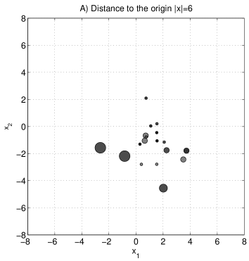
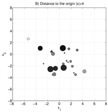
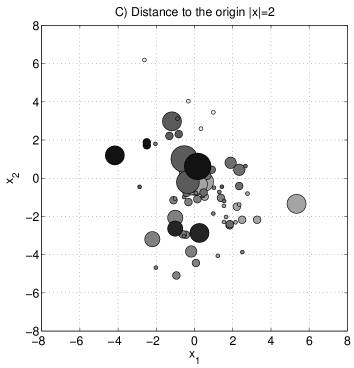
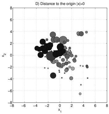
Figure 1: Example of a 3D model population. Different panels show 2D subspaces of the model 3D space at different distances $|{\bf x}|$ to the origin. Model parameters are $\mu=\lambda=1$, $D=1$, $B=2$. Circle size is proportional to the particle rank. Different shades correspond to populations from different immigrants; the descendants of earlier immigrants have lighter shade. The clustering of particles is explained by the splitting histories. Note that, as the origin approaches, the particle activity significantly changes, indicating the increased probability of an extreme event.

As the observation subspace approaches the source, intensity of the observed events increases, larger events become relatively more frequent, clustering and long-range correlations become more prominent (see Fig. 1 and Sects. IV,VIII). Emergence of these patterns, each individually and all together, can be therefore used to forecast an approach of a large event; indeed, such a prediction should be understood in a statistical sense. This study is focused on quantitative description of two of these patterns, intensity increase and deviations from self-similarity, for a classical branching process formally introduced in the next section.

We emphasize that the location and dynamics of the observation space $\mathcal{R}_{t}$ within $\Omega$ depend on details of a particular system of interest and may be hard to estimate or model. An important result of this paper is that (i) the information about this unknown dynamics can be summarized by a scalar value of the control parameter (distance between the observational subspace and the origin); and (ii) knowledge of the control parameter is sufficient to solve the prediction problem.

Finally, it is important to mention that we do not use direct cascade as a dynamical model of event formation, which would imply that large events cause smaller ones. We merely use this analytically tractable approach to create a hierarchical network of spatially distributed particles. A dynamic interpretation of the latter will depend on a concrete application, and may include inverse cascading or other physically relevant processes.

III Model formulation

We consider an age-dependent multi-type branching diffusion process with immigration in $\mathbb{R}^{n}$. The system consists of particles, each of which belongs to a generation $k=0,1,\dots$. Particles of zero generation (the largest ones) appear in a system as a result of external driving (forcing); we will refer to them as immigrants. Particles of any other generation $k>0$ are produced as a result of splitting of particles of generation $k-1$. Immigrants ($k=0$) are born at the origin ${\bf x}:=(x_{1},\dots,x_{n})={\bf 0}$ at a constant rate $\mu$; that is, the probability for a new immigrant to appear within the time interval of length $\Delta t$ is $\mu\Delta t+o(\Delta t)$ as $\Delta t\to 0$. Accordingly, the birth instants form a homogeneous Poisson process with intensity $\mu$. Each particle lives for some random time $\tau$ and then transforms (splits) into a random number $\beta$ of particles of the next generation. The probability laws of the lifetime $\tau$ and branching $\beta$ are generation-, time-, and space-independent. We assume that new particles are born at the location of their parent at the moment of splitting.

The particle lifetime has an exponential distribution:

$$G(t):=\mathsf{P}\{\tau<t\}=1-e^{-\lambda\,t},~{}\lambda>0.$$ (III.1)

The conditional probability that a particle transforms into $k\geq 0$ new particles (0 means that it disappears) given that the transformation took place is denoted by $p_{k}$. The probability generating function (pgf) for the number $\beta$ of new particles is thus

$$h(s)=\sum_{k}p_{k}\,s^{k}.$$ (III.2)

The expected number of offsprings (also called the branching number) is $B:=E(\beta)=h^{\prime}(1)$ (see e.g., AN04 , Chapter 1).

Each particle diffuses in $\mathbb{R}^{n}$ independently of other particles. This means that the density $p({\bf x,y},t)$ of a particle that was born at instant $0$ at point ${\bf y}$ solves the equation

$$\frac{\partial p}{\partial t}=D\left(\sum_{i}\frac{\partial^{2}}{\partial x_{i}^{2}}\right)p\equiv D\bigtriangleup_{{\bf x}}p$$ (III.3)

with the initial condition $p({\bf x,y},0)=\delta({\bf x-y})$. The solution of (III.3) is given by Eva98

$$p({\bf x,y},t)=\left(4\,\pi\,D\,t\right)^{-n/2}\exp\left\{-\frac{|{\bf x-y}|^{2}}{4\,D\,t}\right\},\quad|{\bf x}|^{2}=\sum_{i}x_{i}^{2}.$$ (III.4)

Accordingly, the density of each particle, given that it is alive at the instant $t$, is $\phi({\bf x},t):=p({\bf x},{\bf 0},t)$. Naturally, the positions of the particles produced by the same immigrant are correlated. This can be reflected by the joint distribution of pairs, triplets, etc.

The model is specified by the following parameters: immigration intensity $\mu>0$, branching intensity $\lambda>0$, diffusion constant $D>0$, and branching distribution $\{p_{k}\}$, which will be often represented by its pgf $h(z)$ or simply by the branching number $B$. An appropriate choice of the temporal and spatial scales allows one to assume $\mu=1$ and $D=1$.

It is convenient to introduce particle rank $r:=r_{\rm max}-k$ for an arbitrary integer $r_{\rm max}$ and thus consider particles of ranks $r\leq r_{\rm max}$. Particle rank can be considered a logarithmic measure of the size. Similar to the analysis of the real-world systems, we sometime only consider particles of the first several generations $0\leq k\leq r_{\rm max}-1$, which corresponds to the largest ranks $1\leq r\leq r_{\rm max}$. Figure 1 illustrates the model population.

IV Summary of results related to prediction

We summarize here the study’s findings that are most relevant to the prediction problem. Recall that the prediction problem consists of assessing the likelihood of an extreme event; the latter corresponds to an instant when a sufficiently large particle crosses the observation space. The likelihood of an extreme event is thus directly related to the distance between the space of observations and the origin. Accordingly, the prediction problem is reduced to the estimation of this distance from available data. For that, one should look for increase in the intensity of medium-to-large-sized events, as well as upward deviations in the event size distribution. We believe that this general idea can be useful in a wide range of models and observed systems, not necessarily based on a branching diffusion mechanism. Statistical assessment of particular prediction schemes based on this idea is left for a future study.

All statements below refer to a steady-state of the model (dynamics after a transient). All asymptotic statements have been confirmed numerically in finite models.

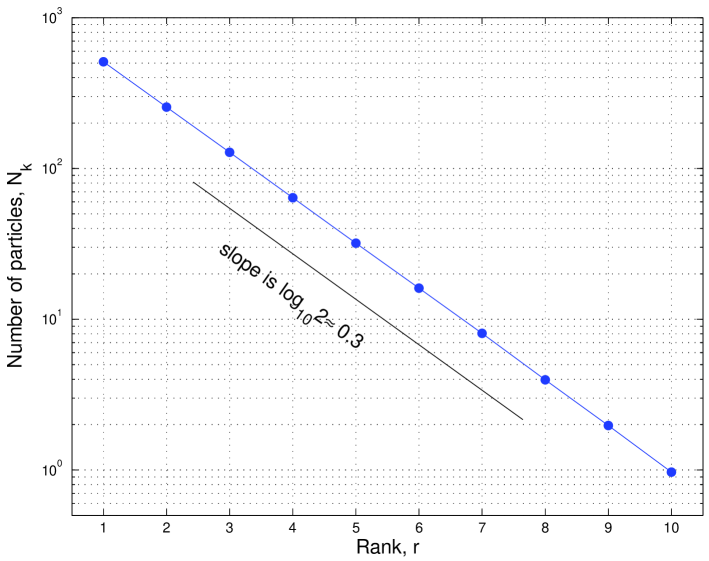
Figure 3: Spatially averaged particle rank distribution at $t=30$. The distribution is averaged over 4000 independent realizations of a 3D model with parameters $\mu=\lambda=1$, $D=1$, $B=2$, $r_{\rm max}=10$. One can clearly see the exponential rank distribution of Eq. (VI.1).

• Meanfield self-similarity. Particle ranks, averaged over time and space, have an exponential distribution; this is equivalent to a power-law distribution of particle sizes; see (VI.1) and Fig. 3.

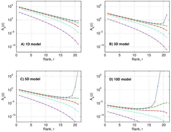
Figure 2: Expected number $A_{k}(z)$ of generation $k$ particles at distance $z$ from the origin (cf. Proposition VI.2). The distance $z$ is increasing (from top to bottom line in each panel) as $z=10^{-3},2,5,10,20$. Model dimension is $n=1$ (panel A), $n=3$ (panel B), $n=5$ (panel C), and $n=10$ (panel D). Other model parameters: $\mu=\lambda=1$, $D=1$, $B=2$, $r_{\rm max}=21$. One can clearly see the transition from downward to upward deviation of the rank distributions from the pure exponential form as we approach the origin. Notably, the magnitude of the upward deviation close to the origin (the upper line in all panels) strongly increases with the model dimension $n$.

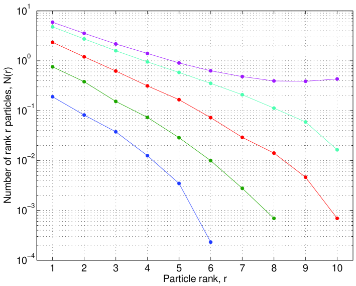
Figure 4: Particle rank distribution at $t=30$ and fixed distance $z$ from the origin (cf. Proposition VI.2). The distribution is averaged over 4000 independent realizations of a 3D model with parameters $\mu=\lambda=1$, $D=1$, $B=2$, $r_{\rm max}=10$. Different lines correspond to different distances (from top to bottom): $z=0,2,4,6,8$. Spatial averaging is done within spherical shells of constant volume $V=5$ with inner radius $z$. One can clearly see that the rank distribution deviates from the pure exponential form, which corresponds to a straight line in the semilogarithmic scale used here. One observes downward deviations at large distances from the origin, and upward deviations close to the origin.

• Small-size self-similarity. The particle rank distribution at any spatial point is asymptotically exponential as rank decreases, with the exponent index $-B$; see (VI.8) and Figs. 2 and 4. This is equivalent to a power-law distribution of particle sizes with power-law index $-B$. Furthermore, this implies that deviations from self-similarity, if any, can be only seen at large ranks (large particle sizes).

• Upward deviations close to the origin. At any point sufficiently close to the origin, the particle size distribution deviates from a self-similar power-law form as to have a larger number of medium-to-large-sized events. The magnitude of this deviation increases with the event size, as well as with dimension of the model space; see (VI.6) and the upper lines in Figs.  2 and 4.

• Downward deviations away from the origin. At any point sufficiently far from the origin, the particle size distribution deviates from a self-similar power-law form as to have a smaller number of medium-to-large-sized events. The magnitude of this deviation increases with the event size and is independent of the model’s dimension; see (VI.7) and the lower lines in Figs. 2 and 4.

• Exponential decay of event intensity. The intensity of events of any fixed size is exponentially decaying away from the origin; see (V.24).

• Divergence of event intensity at the origin. For models with spatial dimension larger than 1, the intensity of sufficiently large events diverges at the origin in a power-law fashion; see (V.24),(V.26) and Fig. 3(b,c,d).

V Model solution: Moment generating functions

The model introduced in Sect. III is a superposition of independent branching processes generated by individual immigrants. Sections V.1 and V.2 analyze, respectively, the one-point and two-point moments of a particle distribution produced by a single immigrant. Then we expand these results to the case of multiple immigrants in Sect. V.3.

V.1 Single immigrant: One-point properties

V.1.1 Moment generating functions

Let $p_{k,i}(G,\textbf{y},t)$ be the conditional probability that at time $t\geq 0$ there exist $i\geq 0$ particles of generation $k\geq 0$ within spatial region $G\subset\mathbb{R}^{n}$ given that at time 0 a single immigrant was injected at point y. The corresponding moment generating function is

$$M_{k}(G,{\bf y},t;s)=\sum_{i}p_{k,i}(G,{\bf y},t)e^{si}.$$ (V.1)

Proposition V.1

The moment generating functions $M_{k}(G,{\bf y},t;s)$ solve the following recursive system of non-linear partial differential equations:

$$\frac{\partial}{\partial t}M_{k}(G,{\bf y},t;s)=D\Delta_{{\bf y}}M_{k}-\lambda M_{k}+\lambda\,h(M_{k-1}),\quad k\geq 1,$$ (V.2)

with initial conditions $M_{k}(G,{\bf y},0;s)\equiv 1$, $k\geq 1$, and

$$M_{0}(G,{\bf y},t;s)=(1-P)+Pe^{s},\quad P:=e^{-\lambda t}\int_{G}p({\bf x},{\bf y},t)d{\bf x}.$$ (V.3)

Here $h(s)$ is defined by (III.2) and $\Delta_{{\bf y}}=\sum_{i}\partial^{2}/\partial y_{i}^{2}.$

Proof is given in Appendix A.

V.1.2 The first moment densities

Let $\bar{A}_{k}(G,{\bf y},t)$ be the expected number of generation-$k$ particles at instant $t$ within the region $G$, produced by a single immigrant injected at point ${\bf y}$ at time $t=0$. It is given by the following partial derivative (see e.g., AN04 , Chapter 1):

$$\bar{A}_{k}(G,{\bf y},t):=\frac{\partial M_{k}(G,{\bf y},t;s)}{\partial s}\Big{|}_{s=0}.$$ (V.4)

Consider also the expectation density $A_{k}({\bf x},{\bf y},t)$ that satisfies, for any $G\subset\mathbb{R}^{n}$,

$$\bar{A}_{k}(G,{\bf y},t)=\int_{G}A_{k}({\bf x},{\bf y},t)d{\bf x}.$$ (V.5)

Corollary V.2

The first moment densities $A_{k}({\bf x},{\bf y},t)$ solve the following recursive system of partial differential equations:

$$\frac{\partial A_{k}({\bf x},{\bf y},t)}{\partial t}=D\Delta_{{\bf x}}A_{k}-\lambda A_{k}+\lambda BA_{k-1},\quad k\geq 1,$$ (V.6)

with the initial conditions $A_{k}({\bf x},{\bf y},0)\equiv 0$, $k\geq 1$,

$$A_{0}({\bf x},{\bf y},0)=\delta({\bf y}-{\bf x}),\quad A_{0}({\bf x},{\bf y},t)=e^{-\lambda t}p({\bf x},{\bf y},t),\>t>0.$$ (V.7)

The solution to this system is given by

$$A_{k}({\bf x},{\bf y},t) = \frac{(\lambda Bt)^{k}}{k!}A_{0}({\bf x},{\bf y},t)$$ (V.8)

$$= \frac{(\lambda B)^{k}}{k!(4\pi D)^{n/2}}t^{k-n/2}\,\exp\left\{-\lambda t-\frac{|{\bf x}-{\bf y}|^{2}}{4Dt}\right\}.$$

Proof is given in Appendix C. It follows from a general result for the higher moments obtained in Appendix B.

The system (V.6) has a transparent intuitive meaning. The rate of change of the expectation density $A_{k}({\bf x},{\bf y},t)$ is affected by the three processes: diffusion of the existing particles of generation $k$ (the first term in the rhs of (V.6)), splitting of the existing particles of generation $k$ at the rate $\lambda$ (the second term), and splitting of the generation $k-1$ particles that produce on average $B$ new particles of generation $k$ (the third term).

To obtain the solution for the entire population, we sum up the contributions from all generations:

$$A({\bf x},{\bf 0},t)=\sum_{k=0}^{\infty}A_{k}({\bf x},{\bf 0},t)=e^{-\lambda\,t\,(1-B)}\,p({\bf x},{\bf 0},t)=\frac{e^{-\lambda\,t\,(1-B)}}{\left(4\,\pi\,D\,t\right)^{n/2}}\exp\left(-\frac{|{\bf x}|^{2}}{4\,D\,t}\right).$$ (V.9)

This formula emphasizes the role of the branching parameter $B$: in subcritical case, $B<1$, the population extincts exponentially; in supercritical case, $B>1$, the population grows exponentially; in critical case, $B=1$, the expected number of particles remains the same (steady state) and is given by the diffusion density $p({\bf x},{\bf 0},t)$.

V.2 Single immigrant: Two-point properties

V.2.1 Moment generating functions

Let $p_{k_{1},k_{2},i,j}(G_{1},G_{2},\textbf{y},t)$ be the conditional probability that at instant $t\geq 0$ there exist $i\geq 0$ particles of generation $k_{1}\geq 0$ within region $G_{1}\subset\mathbb{R}^{n}$ and $j\geq 0$ particles of generation $k_{2}\geq 0$ within region $G_{2}\subset\mathbb{R}^{n}$ given that at time 0 a single immigrant was injected at point y. Assume that $G_{1}$ and $G_{2}$ do not overlap. The corresponding moment generating function is

$$M_{k_{1},k_{2}}\left(G_{1},G_{2},{\bf y},t;s_{1},s_{2}\right)=\sum_{i,j\geq 0}p_{k_{1},k_{2},i,j}(G_{1},G_{2},\textbf{y},t)e^{i\,s_{1}+j\,s_{2}}.$$ (V.10)

Proposition V.3

The moment generating functions $M_{k_{1},k_{2}}\left(G_{1},G_{2},{\bf y},t;s_{1},s_{2}\right)$ solve the following recursive system of non-linear partial differential equations:

$$\frac{\partial}{\partial t}M_{k_{1},k_{2}}=D\Delta_{{\bf y}}M_{k_{1},k_{2}}-\lambda M_{k_{1},k_{2}}+\lambda\,h(M_{k_{1}-1,k_{2}-1}),\quad k_{1},k_{2}\geq 1,$$ (V.11)

with the initial conditions

$$M_{k_{1},k_{2}}\left(G_{1},G_{2},{\bf y},0;s_{1},s_{2}\right)\equiv 1,\quad k_{1},k_{2}\geq 1,$$ (V.12)

$$M_{0,0}\left(G_{1},G_{2},{\bf y},t;s_{1},s_{2}\right)=P_{1}e^{s_{1}}+P_{2}e^{s_{2}}+1-P_{1}-P_{2},$$ (V.13)

$$M_{0,k}\left(G_{1},G_{2},{\bf y},t;s_{1},s_{2}\right)=\big{(}M_{k}(G_{2},{\bf y},t;s_{2})-e^{-\lambda t}\big{)}+(e^{-\lambda t}-P_{1})+P_{1}e^{s_{1}},$$ (V.14)

where $P_{i}:=e^{-\lambda t}\int_{G_{i}}p({\bf x},{\bf y},t)d{\bf x}$, $i=1,2$. Here, as before, $h(s)$ is defined by (III.2) and $\Delta_{{\bf y}}=\sum_{i}\partial^{2}/\partial y_{i}^{2}.$

Proof is given in Appendix D.

V.2.2 Moments

Consider the expected value $\bar{A}_{k_{1},k_{2}}(G_{1},G_{2},\textbf{y},t)$ of the product of the number of generation-$k_{1}$ particles in region $G_{1}$ and number of generation-$k_{2}$ particles in region $G_{2}$ at instant $t$, produced by a single immigrant injected at point y at time $t=0$. It is given by the following partial derivative

$$\bar{A}_{k_{1},k_{2}}(G_{1},G_{2},\textbf{y},t):=\left.\frac{\partial^{2}M_{k_{1},k_{2}}\left(G_{1},G_{2},\textbf{y},t;s_{1},s_{2}\right)}{\partial s_{1}\partial s_{2}}\right|_{s_{1}=s_{2}=0}.$$ (V.15)

We notice that the expectations $\bar{A}_{k_{1}}(G_{1},\textbf{y},t)$ and $\bar{A}_{k_{2}}(G_{2},\textbf{y},t)$ of (V.4) can be represented as

$$\bar{A}_{k_{1}}(G_{1},\textbf{y},t) := \left.\frac{\partial M_{k_{1},k_{2}}\left(G_{1},G_{2},\textbf{y},t;s_{1},s_{2}\right)}{\partial s_{1}}\right|_{s_{1}=s_{2}=0}$$ (V.16)

and

$$\bar{A}_{k_{2}}(G_{2},\textbf{y},t) := \left.\frac{\partial M_{k_{1},k_{2}}\left(G_{1},G_{2},\textbf{y},t;s_{1},s_{2}\right)}{\partial s_{2}}\right|_{s_{1}=s_{2}=0}.$$ (V.17)

Consider also the expectation density $A_{k_{1},k_{2}}(\mathbf{x_{1}},\mathbf{x_{2}},\textbf{y},t)$ that satisfies, for any nonoverlapping $G_{1},G_{2}\subset\mathbb{R}^{n}$

$$\bar{A}_{k_{1},k_{2}}(G_{1},G_{2},\textbf{y},t)=\int_{G_{2}}\int_{G_{1}}A_{k_{1},k_{2}}(\mathbf{x_{1}},\mathbf{x_{2}},\textbf{y},t)d\mathbf{x_{1}}d\mathbf{x_{2}}.$$ (V.18)

Corollary V.4

The moment densities $A_{k_{1},k_{2}}\equiv A_{k_{1},k_{2}}({\bf x_{1}},{\bf x_{2}},{\bf y},t)$ solve the following recursive system of partial differential equations:

$$\frac{\partial A_{k_{1},k_{2}}}{\partial t}=D\,\Delta_{{\bf y}}A_{k_{1},k_{2}}-\lambda\,A_{k_{1},k_{2}}+\lambda\,B\,A_{k_{1}-1,k_{2}-1}$$ (V.19)

$$+ \lambda\,h^{{}^{\prime\prime}}(1)\,A_{k_{1}-1}({\bf x_{1}})\,A_{k_{2}-1}({\bf x_{2}}),\quad k_{1},k_{2}\geq 1,$$

with the initial conditions

$$A_{k_{1},k_{2}}({\bf x_{1}},{\bf x_{2}},{\bf y},0) \equiv 0,\quad k_{1},k_{2}\geq 1,$$ (V.20)

$$A_{0,k}({\bf x_{1}},{\bf x_{2}},{\bf y},t) \equiv 0,\quad k\geq 0,\>t\geq 0,$$ (V.21)

and $A_{k}({\bf x})\equiv A_{k}({\bf x},{\bf y},t)$ given by (V.8).

Proof is given in Appendix E.

V.3 Multiple immigrants

Here we expand the results of the Sect. V.1 to the case of multiple immigrants that appear at the origin according to a homogeneous Poisson process with intensity $\mu$. The expectation ${\mathcal{A}}_{k}$ of the number of particles of generation $k$ is given by

$${\mathcal{A}}_{k}({\bf x},t) = \int_{0}^{t}A_{k}({\bf x},{\bf 0},s)\,\mu\,ds$$ (V.22)

$$= \frac{\mu\,(\lambda\,B)^{k}}{k!\left(4\,\pi\,D\right)^{n/2}}\int_{0}^{t}s^{k-n/2}\,\exp\left\{-\lambda\,s-\frac{|{\bf x}|^{2}}{4\,D\,s}\right\}ds.$$

The steady-state spatial distribution corresponds to the limit $t\to\infty$:

$${\mathcal{A}}_{k}({\bf x}):={\mathcal{A}}_{k}({\bf x},\infty)=\frac{2\,\mu\,(\lambda\,B)^{k}}{k!\left(4\,\pi\,D\right)^{n/2}}\left(\frac{|{\bf x}|^{2}}{4\,D\,\lambda}\right)^{\nu/2}K_{\nu}\left(|{\bf x}|\sqrt{\frac{\lambda}{D}}\right).$$ (V.23)

Here $\nu=k-n/2+1$ and $K_{\nu}$ is the modified Bessel function of the second kind (see Appendix G). Introducing the normalized distance from the origin $z:=|{\bf x}|\sqrt{\lambda/D}$ we obtain

$${\mathcal{A}}_{k}(z)=\frac{\mu}{\lambda\,k!}\left(\frac{B}{2}\right)^{k}\left(\frac{2\,\pi\,D}{\lambda}\right)^{-n/2}\,z^{\nu}\,K_{\nu}(z).$$ (V.24)

For odd $n$, there are explicit expressions for $K_{\nu}(z)$ (Appendix G, Eqs. (G.2),(G.3)). In particular, we have

$${\mathcal{A}}_{0}(z)=\frac{\mu}{\sqrt{4\,D\,\lambda}}e^{-z},{\rm~{}for~{}}n=1,\quad{\mathcal{A}}_{0}(z)=\sqrt{\frac{\lambda}{D^{3}}}\,\frac{\mu}{4\,\pi\,z}e^{-z},{\rm~{}for~{}}n=3.$$ (V.25)

From (V.24) and the asymptotic behavior of $K_{\nu}(z)$ as $z\to 0$ (Appendix G, Eq. (G.5)) it follows that

$$\lim_{z\to 0}\,{\mathcal{A}}_{k}(z)=\left\{\begin{array}[]{cc}\infty,&{\rm for~{}}\nu\leq 0,{~{}i.e.,~{}}k\leq n/2-1\\ const<\infty,&{\rm for~{}}\nu>0,{~{}i.e.,~{}}k>n/2-1.\end{array}\right.$$ (V.26)

Thus, in a model with spatial dimension $n\geq 2$, the elements of several lowest generations $(k\leq n/2-1)$ have an infinite concentration at the origin.

V.4 Alternative model representation

In this section we derive a system of equations for the steady-state expectations ${\mathcal{A}}_{k}({\bf x})$ using the radial symmetry of the problem. By integrating the equation (V.6) from $t=0$ to $\infty$, we obtain

$$D\Delta_{\mathbf{x}}\mathcal{A}_{k}({\bf x})-\lambda\mathcal{A}_{k}({\bf x})+\lambda B\mathcal{A}_{k-1}({\bf x})=0$$

since $A_{k}(\mathbf{x},\mathbf{y},\infty)=0$. We now rewrite this equation in terms of the normalized distance from the origin, $z:=|\mathbf{x}|\sqrt{\lambda/D}$, using the fact that ${\mathcal{A}}_{k}({\bf x})\equiv{\mathcal{A}}_{k}(z)$ as soon as $|{\bf x}|=|z|$:

$$\mathcal{A}_{k}^{{}^{\prime\prime}}(z)+\frac{n-1}{z}\;\mathcal{A}_{k}^{{}^{\prime}}(z)-\mathcal{A}_{k}(z)+B\mathcal{A}_{k-1}(z)=0.$$ (V.27)

We notice, furthermore, that one can rewrite the expectation densities (V.8) as a function of $z$, which results in $A_{k}(z)\equiv A_{k}({\bf x},{\bf 0},t)$. It is then readily seen that

$$A_{k}^{{}^{\prime}}(z)=-\frac{B}{2k}\;z\;A_{k-1}(z).$$ (V.28)

The same recursive system holds for $\mathcal{A}_{k}(z)$, which is shown by integrating the last equation with respect to time.

VI Particle rank distribution

We analyze here the particle rank distribution; recall that the rank is defined as $r=r_{\rm max}-k$, where $k$ is the particle’s generation. A self-similar branching mechanism that governs our model suggests an exponential distribution of particle ranks. Indeed, the spatially averaged steady-state rank distribution is a pure exponential law with index $B$:

$$A_{k}: = \int_{{\mathbb{R}}^{n}}\int_{0}^{\infty}A_{k}({\bf x,0},t)\mu\,dt\,d{\bf x}$$ (VI.1)

$$= \frac{\mu\,B^{k}}{k!}\int_{0}^{\infty}(\lambda\,t)^{k}\,e^{-\lambda\,t}\,dt=\frac{\mu}{\lambda}\,B^{k}\propto B^{-r}.$$

Remark VI.1

Our use of the term “self-similar” with respect to the exponential distribution, often seen in physical literature, requires some explanations. As we mentioned earlier, the particle rank serves as a logarithmic measure of its size. Thus, the exponential distribution of ranks corresponds to the power law distribution of sizes; hence the term “self-similarity”.

To analyze rank- and space-dependent deviations from the pure exponential distribution, we will consider the ratio $\gamma_{k}({\bf x})$ between the number of particles of two consecutive generations:

$$\gamma_{k}({\bf x}):=\frac{{\mathcal{A}}_{k}({\bf x})}{{\mathcal{A}}_{k+1}({\bf x})}.$$ (VI.2)

For the purely exponential rank distribution, $A_{k}({\bf x})=c\,B^{k}$, the value of $\gamma_{k}({\bf x})=1/B$ is independent of $k$ and ${\bf x}$; while deviations from the pure exponential distribution will cause $\gamma_{k}$ to vary as a function of $k$ and/or ${\bf x}$. Plugging (V.24) into (VI.2) we find

$$\gamma_{k}({\bf x})=\frac{2\,(k+1)}{B\,z}\,\frac{K_{\nu}(z)}{K_{\nu+1}(z)},$$ (VI.3)

where, as before, $z:=|{\bf x}|\,\sqrt{\lambda/D}$ and $\nu=k-n/2+1$.

Proposition VI.2

The asymptotic behavior of the function $\gamma_{k}(z)$ is given by

$$\lim\limits_{z\to 0}\gamma_{k}(z) = \left\{\begin{array}[]{cc}\infty,&\nu\leq 0,\\ \displaystyle\frac{1}{B}\left(1+\frac{n}{2\,\nu}\right),&\nu>0,\end{array}\right.$$ (VI.6)

$$\gamma_{k}(z) \sim \frac{2(k+1)}{B\,z},\quad{z\to\infty},\quad{\rm fixed~{}}k,$$ (VI.7)

$$\gamma_{k}(z) \sim \frac{1}{B}\left(1+\frac{n}{2\,\nu}\right),\quad{k\to\infty},\quad{\rm fixed~{}}z.$$ (VI.8)

Proof and explicit rates of divergence in (VI.6) are given in Appendix F.

Proposition VI.2 describes the spatio-temporal deviations of the particle rank distribution from the pure exponential law (VI.1). We interpret below each of the equations (VI.6)-(VI.8) in some detail. Eq. (VI.8) implies that at any spatial point, the distribution asymptotically approaches the exponential form as generation $k$ increases (rank $r$ decreases). In other words, the distribution of small ranks (large generation numbers) is close to the exponential with index $-B$; thus the deviations can only be observed at the largest ranks (small generation numbers). Analysis of the large-rank distribution is done using Eqs. (VI.6) and (VI.7). Near the origin, where the immigrants enter the system, Eq. (VI.6) implies that $\gamma_{k}(z)>\gamma_{k+1}(z)>1/B$ for $\nu>0$. Hence, one observes the upward deviations from the pure exponential distribution: for the same number of rank $r$ particles, the number of rank $r+1$ particles is larger than predicted by the exponential law. The same behavior is in fact observed for $\nu\leq 0$ (see Appendix F, Eq. (F.5)). In addition, for $\nu\leq 0$ the ratios $\gamma_{k}(z)$ do not merely deviate from $1/B$, but diverge to infinity at the origin. Away from the origin, according to Eq. (VI.7), we have $\gamma_{k}(z)<\gamma_{k+1}(z)<1/B$, which implies downward deviations from the pure exponent: for the same number of rank $r$ particles, the number of rank $r+1$ particles is smaller than predicted by the exponential law.

Figure 2 illustrates the above findings; it shows the distribution of particles for the largest ranks at different distances from the origin. One can clearly see the transition from downward to upward deviation of the rank distributions from the pure exponential form as we approach the origin. Notably, the magnitude of the upward deviation close to the origin (the upper line in all panels) strongly increases with the model dimension $n$.

VII Numerical analysis

Our analytical results and asymptotics are closely reproduced in numerical experiments with finite number of generations, limited spatial extent, and spatial averaging (unavoidable when working with observations). Here, to mimic the ensemble averaging, the numerical results have been averaged over 4000 independent realizations of a 3D model with parameters $\mu=\lambda=1$, $D=1$, and $B=2$.

First, we check the exponential rank distribution of (VI.1). Figure 3 shows the observed spatially averaged particle rank distribution. The exponential form (VI.1) is indeed well reproduced.

Next, we see how the spatial averaging affects the rank distribution. Figure 4 shows the rank distribution at $t=30$ at various distances to the origin. The spatial averaging has been done within spherical shells (space between two concentric spheres) of a constant volume $V=5$. Thus, here we see an observable counterpart of the theoretical distributions shown in Fig. 2b. Although the spatial averaging somewhat tapers off the upward bend at the largest ranks close to the origin, the predicted transition from the downward to upward bend is clearly seen.

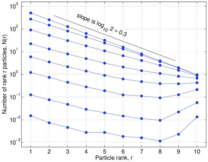
Figure 5: Particle rank distribution at $t=30$ in a 3D model. The distribution is spatially averaged over spheres of volume $V$ centered at the origin with (from top to bottom): $V=\infty,500,100,200,5,1,0.01$. Model parameters: $\mu=\lambda=1$, $D=1$, $B=2$, $r_{\rm max}=10$. The upward deviations from the exponential distribution (a straight line) are fading away with the extent of the spatial averaging.

Figure 5 illustrates in more detail how the spatial averaging affects the upward bend in a 3D model. It shows the particle rank distributions at $t=30$ spatially averaged over spheres of different volumes centered at the origin. The upward bend is prominent for the spheres with volumes $V\leq 5$; and it gradually disappears within larger spheres in favor of an exponential distribution observed after a complete spatial averaging. Notably, the pure exponential distribution can be only achieved by averaging over all events in the model ($V=\infty$).

VIII Discussion

This work is motivated by the problem of prediction of extreme events in complex systems. Our point of departure is the four types of premonitory patterns KB02 , previously found in models and observations. We propose here a simple mechanism and a single control parameter for all these patterns.

Quantitative analysis is performed here for a classical model of spatially distributed population of particles of different sizes governed by direct cascade of branching and external driving (see Sect. III). In the probability theory this model is known as the age-dependent multitype branching diffusion process with immigration AN04 . We consider here a new scope of problems for this model. We assume that observations (detection of particles) are only possible on a subspace of the system space while the source of external driving (origin) remains unobservable, as is the case in many real-world systems. The natural question under this approach is the dependence of the process statistics on the distance to the source. A complete analytical solution to this problem, in terms of the moments with respect to the particle density, is given by Proposition V.1. In addition, the correlation structure of the particle field can be found using Proposition V.3.

It is natural to consider rank as a logarithmic measure of the particle size. The exponential rank distribution derived in Eq. (VI.1) corresponds to a self-similar, power-law distribution of particle sizes, characteristic for many complex systems. The self-similarity in our model, as well as in the real-world systems, is only observed after global spatial averaging in a steady-state. Proposition  VI.2 and Fig. 2 describe space-dependent deviations from the self-similarity. Recall that an extreme event in our system is defined as an observation of a particle of sufficiently large size. As the source approaches the observation subspace, the probability of an extreme event increases. Our results are thus directly connected to prediction: When the location of the source changes in time approaching the subspace of observation (or vice versa), the increase of event intensity and the downward bend in the event size distribution becomes premonitory to an extreme event. The numerical experiments confirm the validity of our analytical results and asymptotics in a finite model.

Our model exhibits very rich and intriguing premonitory behavior. Figure  1 shows several 2D snapshots of a 3D model at different distances from the source. One can see that, as the source approaches, the following changes in the background activity emerge: a) The intensity (total number of particles) increases; b) Particles of larger size become relatively more numerous; c) Particle clustering becomes more prominent; d) The correlation radius increases. All these premonitory changes have been independently observed in natural and socioeconomic systems. Here they are all determined by a single control parameter – distance between the source and the observation space.

The abovementioned premonitory patterns closely resemble universal properties of models of statistical physics in a vicinity of second order phase transition Stanley71 ; Ma00 ; Kadanoff00 , percolation models near the percolation threshold SA94 ; Grimmett , or random graphs prior to the emergence of a giant cluster Bollobas ; Durrett ; NBW06 . In these models, the approach of an extreme event, usually referred to as critical point, and the emergence of premonitory patterns, called critical phenomena, correspond to an instant when a control parameter crosses its critical value. In statistical physics a typical control parameter is temperature or magnetization; in percolation it is the site or bond occupation density; in a random graph — the probability for two vertices to be connected. The theory of critical phenomena Ma00 quantifies system’s behavior at the critical value of the corresponding control parameter. The remarkable power of this theory is connected to the fact that very different systems demonstrate similar behavior near to criticality. More precisely, when the control parameter is close to its critical value, the system sticks to one of just a few types of possible limit behaviors, each being described by an appropriate scale-invariant statistical field theory. In particular, each limit behavior corresponds to the asymptotic power-law size distribution of system observables with a characteristic value of critical exponent.

We focus here on a problem inverse to that considered by the critical phenomena theory: Estimating the deviation of a control parameter from the critical value using the observed system behavior. The motivation for this is coming from environmental, geophysical, and other applied fields where one faces a problem of assessing the likelihood of occurrence of an extreme event associated with a critical point. We formulate and solve such a prediction problem for a spatially embedded cascade process, which enjoys both the mean-field self-similarity and realistic premonitory time- and space-dependent deviations from the latter. The methods developed in this paper may provide a framework for studying predictability of extreme events in complex systems of arbitrary nature.

Appendix A Proof of Proposition V.1

We will need the following calculus lemma that is readily proven by using the definition of derivative:

Lemma A.1

Let $f(z)$, $g(z)$, $z\in\mathbb{R}$ be continuous functions such that the definite integral $G(t)=\int_{0}^{t}f(z)\,g(t-z)dz$ exists. We also assume that $g(z)$ is differentiable. Then,

$$\frac{d}{dt}G(t)=\int_{0}^{t}f(z)\,g^{\prime}(t-z)dz+f(t)\,g(0).$$

There are two possible scenarios for the model development up to time $t$. In the first one, the initial immigrant will not split; the probability for this is $P=e^{-\lambda t}$. In the second one, the initial immigrant will split at instant $0\leq u\leq t$; the probability of the first split within the time interval $[u,u+du]$ is $\lambda e^{-\lambda t}du+o(du)$ as $du\rightarrow 0$. The spatial position of the split is given by the diffusion density $p({\bf x},{\bf y},u)$. If the immigrant splits, the composition property of generating functions gives $M_{k}=h[M_{k-1}]$. Integrating over all possible split instants and locations, we obtain

$$M_{k}(G,{\bf y},t;s)=e^{-\lambda t}+\int_{\mathbb{R}^{n}}d\textbf{y}^{\prime}\int_{0}^{t}du\,\lambda e^{-\lambda u}p(\textbf{y}^{\prime},\textbf{y},u)\,h[M_{k-1}(G,\textbf{y}^{\prime},t-u;s)].$$ (A.1)

Here the first and the second terms correspond to the first and second scenarios, respectively. Using the new integration variable $z=t-u$, we write

$$M_{k}(G,{\bf y},t;s) = e^{-\lambda t}+e^{-\lambda t}\int_{\mathbb{R}^{n}}d\textbf{y}^{\prime}\int_{0}^{t}du\,\lambda e^{\lambda(t-u)}p(\textbf{y}^{\prime},\textbf{y},u)\,h[M_{k-1}(G,\textbf{y}^{\prime},t-u;s)]$$

$$= e^{-\lambda t}\left(1+\int_{\mathbb{R}^{n}}d\textbf{y}^{\prime}\int_{0}^{t}dz\,\lambda e^{\lambda z}p(\textbf{y}^{\prime},\textbf{y},t-z)\;h[M_{k-1}(G,\textbf{y}^{\prime},z;s)]\right).$$

Now we take the derivative with respect to $t$ of both sides and apply Lemma A.1 using the fact that $p(\textbf{y}^{\prime},\textbf{y},0)=\delta(\textbf{y}^{\prime}-\textbf{y})$ and $(\partial/\partial t-D\Delta_{\textbf{y}})p=0:$

$$\frac{\partial}{\partial t}M_{k}(G,\textbf{y},t;s)=-\lambda M_{k}(G,\textbf{y},t;s)\\ +e^{-\lambda t}\left[\int_{\mathbb{R}^{n}}d\textbf{y}^{\prime}\int_{0}^{t}dz\,\lambda e^{\lambda z}\;h[M_{k-1}(G,\textbf{y}^{\prime},z;s)]D\Delta_{\textbf{y}}p(\textbf{y}^{\prime},\textbf{y},t-z)+\lambda e^{\lambda t}\;h[M_{k-1}(G,\textbf{y},t;s)]\right].$$

Taking the operator $\Delta_{\textbf{y}}$ out of the integration signs, we find

$$\frac{\partial}{\partial t}M_{k}(G,\textbf{y},t;s)=D\Delta_{\textbf{y}}M_{k}-\lambda M_{k}+\lambda\;h[M_{k-1}].$$

It is left to establish the initial conditions. Since we start the model with a particle of generation $k=0$ and the distribution of splitting is continuous, at $t=0$ there are no other particles with probability 1. Hence, $M_{k}(G,\textbf{y},0;s)=1$ for all $k\geq 1$. For generation $k=0$, we can only have one or no particles at time $t>0$. The probability to have one particle is given by the product of probabilities that there was no split up to time $t$ and that the particle happens to be within region $G$ at time $t$: $P=e^{-\lambda t}\int_{G}p(\textbf{x},\textbf{0},t)d\textbf{x}$. The probability to have no particles is then $(1-P)$. This implies (V.3). $\Box$

Appendix B Moments in one-point system

For any natural number $j$, consider the $j$-th moment $\bar{A}^{(j)}_{k}(G,{\bf y},t)$ of the number of generation-$k$ particles at instant $t$ within the region $G$, produced by a single immigrant injected at point ${\bf y}$ at time $t=0$. It is given by the following partial derivative (see e.g., AN04 , Chapter 1):

$$\bar{A}^{(j)}_{k}(G,{\bf y},t):=\frac{\partial^{j}M_{k}(G,{\bf y},t;s)}{\partial s^{j}}\Big{|}_{s=0}.$$ (B.1)

Corollary B.1

The moments $\bar{A}_{k}^{(j)}(G,{\bf y},t)$ solve the following recursive system of partial differential equations:

$$\frac{\partial}{\partial t}\bar{A}_{k}^{(j)}(G,\mathbf{y},t)=D\Delta_{\mathbf{y}}\bar{A}_{k}^{(j)}-\lambda\bar{A}_{k}^{(j)}+\lambda\left[\sum\frac{j!}{m_{1}!m_{2}!\dots m_{j}!}h^{(m)}(1)\prod_{i=1}^{j}\left(\frac{\bar{A}_{k-1}^{(i)}}{i!}\right)^{m_{i}}\;\right],$$ (B.2)

where $m=m_{1}+\dots+m_{j}$ and the sum is over all partitions of $j$, i.e., values of $m_{1},\ldots,m_{j}$ such that $m_{1}+2m_{2}+\dots+jm_{j}=j$, with the initial conditions

$$\bar{A}_{k}^{(j)}(G,{\bf y},0) \equiv 0,k\geq 1,$$ (B.3)

$$\bar{A}_{0}^{(j)}(G,{\bf y},0) = \int_{G}\delta(\mathbf{y}-\mathbf{x})d{\bf x},$$ (B.4)

$$\bar{A}_{0}^{(j)}(G,{\bf y},t) = e^{-\lambda t}\int_{G}p(\mathbf{x},\mathbf{y},t)d{\bf x},\;t>0,$$ (B.5)

and

$$h^{(i)}(1):=\left.\frac{d^{i}}{ds^{i}}h(s)\right|_{s=1}=\sum_{n=i}^{\infty}\frac{n!}{(n-i)!}\,p_{n}.$$

Proof: The validity of (B.2) follows from Proposition V.1. Namely, applying the operator $\partial^{j}/\partial s^{j}(\cdot)|_{s=0}$ to both sides of (V.2), changing the order of differentiation, and using Faà di Bruno’s formula for the $j$-th derivative of a composition function, one finds, for each $k\geq 1$,

$$\frac{\partial^{j}}{\partial s^{j}}\left.\left[\frac{\partial M_{k}(G,\textbf{y},t;s)}{\partial t}\right]\right|_{s=0} = \frac{\partial^{j}}{\partial s^{j}}\left[D\Delta_{\bf{y}}M_{k}-\lambda M_{k}+\lambda\,h(M_{k-1})\right]|_{s=0},$$

$$\frac{\partial}{\partial t}\left.\left[\frac{\partial^{j}M_{k}(G,\textbf{y},t;s)}{\partial s^{j}}\right|_{s=0}\right] = \left.\left[D\Delta_{\bf{y}}\frac{\partial^{j}M_{k}}{\partial s^{j}}-\lambda\frac{\partial^{j}M_{k}}{\partial s^{j}}+\lambda\,\frac{\partial^{j}}{\partial s^{j}}h(M_{k-1})\right]\right|_{s=0},$$

$$\frac{\partial}{\partial t}\bar{A}^{(j)}_{k}\left(G,{\bf y},t\right)=\left[D\Delta_{{\bf y}}\frac{\partial^{j}M_{k}}{\partial s^{j}}-\lambda\frac{\partial^{j}M_{k}}{\partial s^{j}}\right.$$

$$+ \left.\left.\lambda\,\left(\sum\frac{j!}{m_{1}!m_{2}!\dots m_{j}!}\,h^{(m)}(M_{k-1})\prod_{i=1}^{j}\left(\frac{M_{k-1}^{(i)}}{i!}\right)^{m_{i}}\right)\right]\right|_{s=0}$$

$$= D\Delta_{\bf y}\bar{A}_{k}^{(j)}-\lambda\bar{A}_{k}^{(j)}+\lambda\left[\sum\frac{j!}{m_{1}!m_{2}!\dots m_{j}!}h^{(m)}(1)\prod_{i=1}^{j}\left(\frac{\bar{A}_{k-1}^{(i)}}{i!}\right)^{m_{i}}\;\right],$$

where $m=m_{1}+\dots+m_{j}$ and the sum is over all partitions of $j$, i.e., values of $m_{1},\ldots,m_{j}$ such that $m_{1}+2m_{2}+\dots+jm_{j}=j$. The initial conditions are established by applying the operator $\partial^{j}/\partial s^{j}(\cdot)|_{s=0}$ to both sides of (V.3) and using the definition of $\bar{A}^{(j)}_{k}(G,\mathbf{y},t)$ in (V.4).

Appendix C Proof of Corollary V.2

For $j=1$, the equation in Corollary B.1 simplifies to

$$\frac{\partial}{\partial t}\bar{A}_{k}(G,\textbf{y},t)=D\Delta_{\textbf{y}}\bar{A}_{k}-\lambda\bar{A}_{k}+\lambda B\bar{A}_{k-1}.$$

Using the definition of $A_{k}(\textbf{x},\textbf{y},t)$ given in (V.5), one obtains for each $k\geq 1$,

$$\frac{\partial}{\partial t}A_{k}(\textbf{x},\textbf{y},t)=D\Delta_{\textbf{y}}A_{k}-\lambda A_{k}+\lambda BA_{k-1}.$$

It is left to use the translation property $A_{k}(\textbf{x},\textbf{y},t)=A_{k}(\textbf{x}-\textbf{y},\textbf{0},t)$ to change $\Delta_{\textbf{y}}$ to $\Delta_{\textbf{x}}$.

The validity of general solution (V.8) is proven by induction using the fact that

$$\left[\frac{\partial}{\partial t}-D\Delta_{\textbf{x}}+\lambda\right]A_{0}=0.$$

The last equality in (V.8) follows from (B.5) and (III.4). $\Box$

Appendix D Proof of Proposition V.3

The proof of Proposition V.3 follows the line of the proof of Proposition V.1. There are two possible scenarios for the model development up to time $t$. In the first one, the initial immigrant will not split; the probability for this is $P=e^{-\lambda t}$. In the second one, the initial immigrant will split at instant $0\leq u\leq t$; the probability of the first split within the time interval $[u,u+du]$ is $\lambda e^{-\lambda t}du+o(du)$ as $du\rightarrow 0$. The spatial position of the split is given by the diffusion density $p(\textbf{x},\textbf{y},u)$. If the immigrant splits, the composition property of generating functions gives $M_{k_{1},k_{2}}=h[M_{k_{1}-1,k_{2}-1}]$. Integrating over all possible split instants and locations, we obtain

$$M_{k_{1},k_{2}}\left(G_{1},G_{2},\textbf{y},t;s_{1},s_{2}\right)\\ =e^{-\lambda t}+\int_{\mathbb{R}^{n}}d\textbf{y}^{\prime}\int_{0}^{t}du\,\lambda e^{-\lambda u}p(\textbf{y}^{\prime},\textbf{y},u)\,h\left[M_{k_{1}-1,k_{2}-1}\left(G_{1},G_{2},\textbf{y}^{\prime},t-u;s_{1},s_{2}\right)\right].$$

Here the first and the second terms correspond to the first and second scenarios, respectively. Using the new integration variable $z=t-u$, we write

$$M_{k_{1},k_{2}}\left(G_{1},G_{2},\textbf{y},t;s_{1},s_{2}\right)\\ =e^{-\lambda t}+e^{-\lambda t}\int_{\mathbb{R}^{n}}d\textbf{y}^{\prime}\int_{0}^{t}du\,\lambda e^{\lambda(t-u)}p(\textbf{y}^{\prime},\textbf{y},u)\,h\left[M_{k_{1}-1,k_{2}-1}\left(G_{1},G_{2},\textbf{y}^{\prime},t-u;s_{1},s_{2}\right)\right]\\ =e^{-\lambda t}\left(1+\int_{\mathbb{R}^{n}}d\textbf{y}^{\prime}\int_{0}^{t}dz\,\lambda e^{\lambda z}p(\textbf{y}^{\prime},\textbf{y},t-z)\,h\left[M_{k_{1}-1,k_{2}-1}\left(G_{1},G_{2},\textbf{y}^{\prime},z;s_{1},s_{2}\right)\right]\right).$$

Now we take the derivative with respect to $t$ of both sides and apply Lemma A.1 using the fact that $p(\textbf{y}^{\prime},\textbf{y},0)=\delta(\textbf{y}^{\prime}-\textbf{y})$ and $(\partial/\partial t-D\Delta_{\textbf{y}})p=0$:

$$\frac{\partial}{\partial t}M_{k_{1},k_{2}}\left(G_{1},G_{2},\textbf{y},t;s_{1},s_{2}\right)=-\lambda M_{k_{1},k_{2}}\left(G_{1},G_{2},\textbf{y},t;s_{1},s_{2}\right)\\ +e^{-\lambda t}\left[\int_{\mathbb{R}^{n}}d\textbf{y}^{\prime}\int_{0}^{t}dz\,\lambda e^{\lambda z}\,h\left[M_{k_{1}-1,k_{2}-1}\left(G_{1},G_{2},\textbf{y}^{\prime},z;s_{1},s_{2}\right)\right]D\Delta_{\textbf{y}}p\left(\textbf{y}^{\prime},\textbf{y},t-z\right)\right.\\ +\left.\lambda e^{\lambda t}\;h\left[M_{k_{1}-1,k_{2}-1}\left(G_{1},G_{2},\textbf{y},t;s_{1},s_{2}\right)\right]\vphantom{\int_{0}^{0}}\right].$$

Taking the operator $\Delta_{\textbf{y}}$ out of the integration signs, we find

$$\frac{\partial}{\partial t}M_{k_{1},k_{2}}\big{(}G_{1},G_{2},\textbf{y},t;s_{1},s_{2}\big{)}=D\Delta_{\textbf{y}}M_{k_{1},k_{2}}-\lambda M_{k_{1},k_{2}}+\lambda\;h[M_{k_{1}-1,k_{2}-1}].$$

It is left to establish the initial conditions. Since we start the model with a particle of generation $k=0$ and the distribution of splitting is continuous, at $t=0$ there are no other particles with probability 1. Hence, $M_{k_{1},k_{2}}\big{(}G_{1},G_{2},\textbf{y},0;s_{1},s_{2}\big{)}=1$ for all $k_{1},k_{2}\geq 1$. For generation $k_{1}=k_{2}=0$, we have three possibilities: the initial immigrant has not split and is in $G_{1}$ ($i=1,j=0$), the initial immigrant has not split and is in $G_{2}$ ($i=0,j=1$), and neither ($i=0,j=0$), with corresponding probabilities of $P_{1}$, $P_{2}$, and $1-P_{1}-P_{2}$, respectively. This implies (V.13).

For generation $k_{1}=0$ and $k_{2}=k\geq 1$, we again have three possibilities: the initial immigrant has not split and is in $G_{1}$ ($i=1,j=0$), the initial immigrant has not split and is not in $G_{1}$ ($i=0,j=0$), and the initial immigrant has split ($i=0,j\geq 0$), with corresponding probabilities of $P_{1}$, $e^{-\lambda t}-P_{1}$, and $1-e^{-\lambda t}$, respectively. In the last case, the number of the $0$-th generation particles in $G_{1}$ is $0$ with probability 1 while the information on the $k$-th generation particles in $G_{2}$ is given by

$$\int_{\mathbb{R}^{n}}d\textbf{y}^{\prime}\int_{0}^{t}du\,\lambda e^{-\lambda u}p(\textbf{y}^{\prime},\textbf{y},u)\;h[M_{k-1}(G_{2},\textbf{y}^{\prime},t-u;s_{2})].$$

From (A.1), we see that the above expression equals $M_{k}(G_{2},\textbf{y},t;s_{2})-e^{-\lambda t}.$ This implies (V.14). We notice that setting $s_{2}=0$ in (V.13) and (V.14) each yields $(1-P_{1})+P_{1}e^{s_{1}}$ as it should (cf. (V.3)). $\Box$

Appendix E Proof of Corollary V.4

The validity of (V.19) follows from Proposition V.3 and the definition of $\bar{A}_{k_{1},k_{2}}(G_{1},G_{2},\mathbf{y},t)$, $A_{k_{1},k_{2}}({\bf x_{1}},{\bf x_{2}},\mathbf{y},t)$. Formally, applying the operator $\partial^{2}/\partial s_{1}\partial s_{2}(\cdot)|_{s_{1}=s_{2}=0}$ to both sides of (V.11) and changing the order of differentiation, one finds, for each $k_{1},k_{2}\geq 1$,

$$\frac{\partial^{2}}{\partial s_{1}\partial s_{2}}\left[\frac{\partial M_{k_{1},k_{2}}}{\partial t}\right]\Big{|}_{s_{1}=s_{2}=0}=\frac{\partial^{2}}{\partial s_{1}\partial s_{2}}\left[D\Delta_{\bf{y}}M_{k_{1},k_{2}}-\lambda M_{k_{1},k_{2}}+\lambda\,h(M_{k_{1}-1,k_{2}-1})\right]\Big{|}_{s_{1}=s_{2}=0},$$

$$\frac{\partial}{\partial t}\left[\frac{\partial^{2}M_{k_{1},k_{2}}}{\partial s_{1}\partial s_{2}}\Big{|}_{s_{1}=s_{2}=0}\right]=\left[D\Delta_{\bf{y}}\frac{\partial^{2}M_{k_{1},k_{2}}}{\partial s_{1}\partial s_{2}}-\lambda\frac{\partial^{2}M_{k_{1},k_{2}}}{\partial s_{1}\partial s_{2}}+\lambda\,h^{{}^{\prime}}(M_{k_{1}-1,k_{2}-1})\frac{\partial^{2}M_{k_{1}-1,k_{2}-1}}{\partial s_{1}\partial s_{2}}\right.$$

$$\qquad\left.+\lambda h^{{}^{\prime\prime}}(M_{k_{1}-1,k_{2}-1})\frac{\partial M_{k_{1}-1,k_{2}-1}}{\partial s_{1}}\,\frac{\partial M_{k_{1}-1,k_{2}-1}}{\partial s_{2}}\right]\Big{|}_{s_{1}=s_{2}=0},$$

$$\frac{\partial}{\partial t}=D\Delta_{\bf{y}}\bar{A}_{k_{1},k_{2}}-\lambda\bar{A}_{k_{1},k_{2}}+\lambda B\bar{A}_{k_{1}-1,k_{2}-1}+\lambda h^{{}^{\prime\prime}}(1)\bar{A}_{k_{1}-1}(G_{1})\bar{A}_{k_{2}-1}(G_{2}).$$

The system (V.19) readily follows now from the definition of $A_{k_{1},k_{2}}({\bf x_{1}},{\bf x_{2}},\mathbf{y},t)$. The initial conditions (V.20) - (V.21) are established by applying the operator $\partial^{2}/\partial s_{1}\partial s_{2}(\cdot)|_{s_{1}=s_{2}=0}$ to both sides of (V.12) - (V.14) and using again the definition of $A_{k_{1},k_{2}}({\bf x_{1}},{\bf x_{2}},\mathbf{y},t)$. $\Box$

Appendix F Proof of Proposition VI.2

The asymptotic (VI.7) readily follows from (G.4). To prove (VI.8), let $r_{\nu}(z):=K_{\nu}(z)/K_{\nu+1}(z)$. From (G.1) one finds that

$$\frac{K_{\nu+1}(z)}{K_{\nu}(z)}=\frac{K_{\nu-1}(z)}{K_{\nu}(z)}+\frac{2\,\nu}{z}$$ (F.1)

and furthermore

$$\frac{z}{2\,\nu}\frac{1}{r_{\nu}(z)}=\frac{z}{2\,\nu}{r_{\nu-1}(z)}+1.$$ (F.2)

From monotonicity of $K_{\nu}(z)$ with respect to the index $\nu>0$ it follows that $r_{\nu}(z)<1$ for $\nu>0$. Accordingly, the first term in the rhs of (F.2) goes to zero as $k\to\infty$. Hence,

$$\lim\limits_{k\to\infty}\frac{z}{2\,\nu}\frac{1}{r_{\nu}(z)}=1,\quad{\rm or}\quad r_{\nu}(z)\sim\frac{z}{2\,\nu},\quad k\to\infty.$$ (F.3)

To complete the proof of (VI.8), we use this asymptotic in (VI.3). Finally, we prove (VI.6). In fact, we will derive a stronger result showing the asymptotics of $r_{\nu}(z)$ and $\gamma_{\nu}(z)$ as $z\to 0$. To find the asymptotics for $r_{\nu}(z)$, we use (G.5) for all possible combinations of signs for $\nu$ and $\nu+1$. We take into account that by definition $\nu$ can only take values $\{i,i+1/2\}_{i\in\mathbb{Z}}$.

$$r_{\nu}(z)=\left\{\begin{array}[]{llllll}\frac{K_{\nu}(z)}{K_{\nu+1}(z)}&\sim&\frac{\Gamma(-\nu)}{\Gamma(-\nu-1)}\left(\frac{2}{z}\right)^{-\nu-(-\nu-1)}&\sim&2\,(-\nu-1)/z,&\nu\leq-3/2,\\ \frac{K_{-1}(z)}{K_{0}(z)}&\sim&[z\,(\ln(2/z)-\gamma)]^{-1}&\sim&\displaystyle-(z\,\ln\,z)^{-1},&\nu=-1,\\ \frac{K_{-1/2}(z)}{K_{1/2}(z)}&&&=&1,&\nu=-1/2,\\ \frac{K_{0}(z)}{K_{1}(z)}&\sim&z\,(\ln(2/z)-\gamma)&\sim&-z\,\ln\,z,&\nu=0,\\ \frac{K_{\nu}(z)}{K_{\nu+1}(z)}&\sim&\frac{\Gamma(\nu)}{\Gamma(\nu+1)}\left(\frac{2}{z}\right)^{\nu-(\nu+1)}&=&z/(2\,\nu),&\nu>0.\end{array}\right.$$ (F.4)

Combining this with (VI.3) we find

$$\gamma_{\nu}(z)=\frac{2\,(k+1)}{B\,z}\,r_{\nu}(z)\sim\left\{\begin{array}[]{cl}\frac{4}{B\,z^{2}}(\nu+n/2)\,(-\nu-1),&\nu\leq-3/2,\\ -\frac{(n-2)}{B\,z^{2}\,\ln\,z},&\nu=-1,\\ \frac{n-1}{B\,z},&\nu=-1/2,\\ -\frac{n\,\ln\,z}{B},&\nu=0,\\ \frac{1}{B}\left(1+\frac{n}{2\,\nu}\right),&\nu>0.\end{array}\right.$$ (F.5)

One can see that for $\nu\leq 0$ the ratio $\gamma_{\nu}(z)$ diverges at the origin. The rate of divergence increases monotonously from $\ln\,z$ to $z^{-2}$ with the absolute value of $\nu$.

Appendix G Properties of $K_{\nu}$

Here we summarize some essential facts about the modified Bessel function of the second kind $K_{\nu}(z)$. The sources of this as well as further information about $K_{\nu}(z)$ are handbooks AS , Chapters 9, 10 and GR , Sect. 8.4. The function $K_{\nu}$ can be defined as a decreasing solution of the modified Bessel differential equation

$$x^{2}\,y^{\prime\prime}+x\,y^{\prime}-\left(x^{2}+\nu^{2}\right)\,y=0.$$

The function $K_{\nu}(z)$ exponentially decreases as $z\to\infty$ and diverges at $z=0$. In addition, $K_{-\nu}(z)=K_{\nu}(z)$ and

$$K_{\nu+1}(z)=K_{\nu-1}(z)+\frac{2\,\nu}{z}\,K_{\nu}(z).$$ (G.1)

For integer $k\geq 0$ we have

$$K_{k+1/2}(z)=\sqrt{\frac{\pi}{2z}}e^{-z}\sum_{m=0}^{k}\frac{(k+m)!}{m!(k-m)!(2z)^{m}},$$ (G.2)

and in particular

$$K_{\pm 1/2}(z)=\sqrt{\frac{\pi}{2\,z}}\,e^{-z};\quad K_{3/2}(z)=\sqrt{\frac{\pi}{2\,z^{3}}}\,e^{-z}.$$ (G.3)

For arbitrary fixed $\nu$ and $z\gg\nu$

$$K_{\nu}(z)\sim\sqrt{\frac{\pi}{2\,z}}\,e^{-z},\quad z\to\infty.$$ (G.4)

The asymptotic behavior at $z=0$ is given by

$$K_{\nu}(z)\sim\left\{\begin{array}[]{cc}\displaystyle\frac{\Gamma(|\nu|)}{2}\,\left(\frac{2}{z}\right)^{|\nu|},&|\nu|\neq 0,\\ \displaystyle\log\left(\frac{2}{z}\right)-\gamma,&\nu=0,\end{array}\right.$$ (G.5)

where $\gamma\approx 0.577$ is the Euler-Mascheroni constant.

References

- (1) S. Albeverio, V. Jentsch, and H. Kantz (eds), Extreme Events in Nature and Society (Springer, Heidelberg, 2005).
- (2) V. I. Keilis-Borok and A. A. Soloviev, A. A. (eds), Nonlinear Dynamics of the Lithosphere and Earthquake Prediction (Springer, Heidelberg, 2003).
- (3) D. Sornette, Critical Phenomena in Natural Sciences 2-nd ed. (Springer-Verlag, Heidelberg, 2004).
- (4) N. Wiener, Extrapolation, interpolation and smoothing of stationary time series with engineering applications, (Wiley, 1949).
- (5) A. N. Kolmogorov, Interpolation, extrapolation of stationary random sequences, Izv. Akad. Nauk. SSSR, Ser. Mat., 5, 3-14 (1941). (English translation: W. Doyle, RAND corporation memorandum RM-3090-PR, April 1962).
- (6) R. E. Kalman and R. S. Bucy , ASME Transactions, J. Basic Eng., Series D, 83, 95-108 (1961).
- (7) H. J. Kushner, SIAM J. Control, 2, 106-119 (1962).
- (8) M. Zakai, Warsch. Und Ver. Gebiete, 11, 230-243 (1969).
- (9) A. Doucet, N. de Freitas and N. Gordon (eds), Sequential Monte Carlo Methods in Practice, (Springer, 2001).
- (10) P. L. Chow, Stochastic Partial Differential Equations, (Chapman Hall/CRC Press, Boca Raton, FL, 2007).
- (11) P. Embrechts, C. Klüppelberg, and T. Mikosch, Modelling Extremal Events for Insurance and Finance (Stochastic Modelling and Applied Probability), (Springer, 2008).
- (12) V. I. Keilis-Borok, L. Knopoff, and I. M. Rotwain, Nature 283, 258-263 (1980).
- (13) V. I. Keilis-Borok, Physica D 77, 193-199 (1994).
- (14) V. I. Keilis-Borok, Proc. Natl. Ac. Sci. USA, 93, 3748-3755 (1996).
- (15) V. I. Keilis-Borok, Ann. Rev. Earth Planet. Sci., 30, 1-33 (2002).
- (16) V. I. Keilis-Borok and V. G. Kossobokov, Phys. Earth Planet. Inter. 61 (1-2), 73-83 (1990).
- (17) V. I. Keilis-Borok and P. N. Shebalin (eds.), Phys. Earth Planet. Inter. 111, (1999).
- (18) I. A. Vorobieva, Phys. Earth Planet. Inter. 111, 197-206 (1999).
- (19) K. Aki, Earthquake Prediction Res. 3, 219-230 (1985).
- (20) C. J. Allegre, J. L. Lemouel, and A. Provost, Nature 297, 5861, 47-49 (1982).
- (21) A. Press and C. Allen, J. Geophys. Res. 100, 6421-6430 (1995).
- (22) B. Romanowicz, Science 260, 1923-1926 (1993).
- (23) K. Mogi, in Earthquake Prediction: An International Review, Maurice Ewing Series, 4 (American Geophysical Union, Washington, DC, 1981), 43-51.
- (24) R. E. Haberman, in Earthquake Prediction: An International Review, Maurice Ewing Series, 4 (American Geophysical Union, Washington, DC, 1981), 29-42.
- (25) W. Smith, Nature 289, 136-139 (1981).
- (26) T. Yamashita and L. Knopoff, J. Geophys. Res. 97, 19873-19879 (1992).
- (27) J. Rundle, D. Turcotte, and W. Klein (eds), Geocomplexity and the Physics of Earthquakes. (American Geophysical Union, Washington DC, 2000).
- (28) G. F. Pepke, J. R. Carlson, and B. E. Shaw, J. Geophys. Res. 99, 6769-6788 (1994).
- (29) L. R. Sykes, B. E. Shaw, and C. H. Scholz, Pure Appl. Geophys. 155:2-4, 207-232 (1999).
- (30) D. L. Turcotte, Ann. Rev. Earth Planet. Sci., 19, 263-281 (1991).
- (31) S. C. Jaume and L. R. Sykes, Pure Appl. Geophys., 155 (2-4): 279-305 (1999).
- (32) T. H. Jordan, Seismol. Res. Lett. 77(1), 3-6 (2006).
- (33) D. Lockner, Intl. J. Rock Mech. Mining Sci. Geomech. Abstr. 30, 7, 883-899 (1993).
- (34) G. Molchan, O. Dmitrieva, and I. Rotwain, Phys. Earth and Planet. Inter. 61, 1-2, 128-139 (1990).
- (35) G. Zoeller, S. Hainzl, and J. Kurths, J. Geophys. Res. 106, 2167 2176 (2001).
- (36) M. Eneva and Y. Ben-Zion, J. Geophys. Res. 102, 17785-17795 (1997).
- (37) M. Anghel, Y. Ben-Zion, and R. Rico-Martinez, Pure Appl. Geophys. 161, 9-10, 2023-2051 (2004).
- (38) I. M. Rotwain, V. I. Keilis-Borok, and L. Botvina, Phys. Earth Planet. Inter., 101, 61-71 (1997).
- (39) V. Keilis-Borok, J. H. Stock, A. Soloviev, and P. Mikhalev, J. Forecasting 19, 65 80 (2000).
- (40) V. I. Keilis-Borok, A. A. Soloviev, C. B. Allegre CB, et al. Pattern Recognition 38, (3), 423-435 (2005).
- (41) I. Zaliapin, H. Wong, and A. Gabrielov, Phys. Rev. E, 71, 066118 (2004).
- (42) A. Gabrielov, V. Keilis-Borok, Y. Sinai, and I. Zaliapin, in ESI Lecture Notes in Mathematics and Physics: Boltzmann’s Legacy, G. Gallavotti, W. Reiter and J. Yngvason (Eds.), 203-216.
- (43) E. M. Blanter, M. G. Shnirman, and J. L. LeMouel, Phys. Earth Planet. Inter., 103 (1-2), 135-150 (1997).
- (44) A. M. Gabrielov, I. V. Zaliapin, V. I. Keilis-Borok, and W. I. Newman W. I., Geophys. J. Int., 143, 427-437 (2000).
- (45) G. S. Narkunskaya and M. G. Shnirman, Phys. Earth. Planet. Inter., 61, 29-35 (1990).
- (46) G. S. Narkunskaya and M. G. Shnirman, Computational Seismology and Geodynamics, (AGU, Washington, D.C.), 1, 20-24 (1994).
- (47) W. I. Newman, D. L. Turcotte, and A. M. Gabrielov, Phys. Rev. E, 52, 4827-4835 (1995).
- (48) I. Zaliapin, V. Keilis-Borok, and M. Ghil, J. Stat. Phys., 111, (3-4), 839-861 (2003).
- (49) A. N. Kolmogorov, Dokl. Akad. Nauk. USSR, 30, 299–303, (1941) (in Russian). English translation: Proc. Royal Soc. London, Series A, 434, 9 13 (1991).
- (50) A. N. Kolmogorov, Dokl. Akad. Nauk. USSR, 32, 16–18, (1941) (in Russian). English translation: Proc. Royal Soc. London, Series A, 434, 15 17 (1991).
- (51) A. M. Obukhov, Dokl. Akad. Nauk. USSR, 1, 22–24 (1941).
- (52) U. Frisch, Turbulence: The Legacy of A. M. Kolmogorov, (Cambridge University Press, 1996).
- (53) J. C. McWilliams, J. Fluid Mech., 219, 361–385.
- (54) B. Gutenberg, and C. F. Richter, Geol. Soc. Amer., Special papers 34, 1-131 (1941).
- (55) B. Gutenberg, and C. F. Richter, Bull. Seism. Soc. Am. 34 185-188 (1944).
- (56) Y. Ben-Zion, in International Handbook of Earthquake and Engineering Seismology, Part B, 1857-1875, (Academic Press, 2003).
- (57) G. K. Zipf, Psycho-Biology of Languages, (Houghton-Mifflin, 1935; MIT Press, 1965).
- (58) V. Pareto, Cours d’economie Politique, (F. Rouge, Lausanne, 1897).
- (59) O. S. Klass, O. Biham, M. Levy, O. Malcai, and S. Soloman, Econ. Lett. 90, 2, 290 295 (2006).
- (60) L. F. Richardson, Statistics of deadly quarrels, (Boxwood Pr., 1960).
- (61) A. J. Lotka, J. Washington Ac. Sci. 16 (12), 317-324 (1926).
- (62) B. D. Malamud, D. L. Turcotte, F. Guzzetti, and P. Reichenbach, Earth Planet. Sci. Lett. 229, 1-2, 45-59 (2004).
- (63) M. T. Brunetti, F. Guzzetti, and M. Rossi Nonlin. Proc. Geophys., 16, 2, 179-188 (2009).
- (64) B. Mandelbrot and H. M. Taylor, Operation Res., 15, 6, 1057-1062 (1967).
- (65) V. Plerou, H. E. Stanley, Phys. Rev. E, 77, 3, Art. No. 037101 (2008).
- (66) X. Gabaix, P. Gopikrishnan, V. Plerou, and H. E. Stanley, Nature, 423, (6937), 267-270 (2003).
- (67) B. Burlando, J. Theor. Biol. 146, 99-114 (1990).
- (68) M. E. J. Newman, Physica D, 107, 293-196 (1997).
- (69) M. E. J. Newman, Contemp. Phys., 46 (5), 323-351 (2005).
- (70) R. Albert and A. L. Barabasi, Rev. Modern Phys., 74 (1), 47-97 (2002).
- (71) B. Mandelbrot, The Fractal Geomery of Nature (W. H. Freeman, 1983).
- (72) D. L. Turcotte, Fractals and Chaos in Geology and Geophysics (Cambridge University Press, 2nd ed. 1997).
- (73) P. Bak, C. Tang, and K. Wiesenfeld, Phys. Rev. A, 38, 1, 364-374 (1988).
- (74) D. L. Turcotte, Rep. Prog. Phys., 62, 10,1377-1429 (1999).
- (75) D. Dhar, Phys. Rev. Lett, 64, 14, 1613-1616 (1990).
- (76) B. Drossel, F. Schwabl, Phys. Rev. Lett., 69, 11, 1629-1632 (1992).
- (77) J. B. Rundle and W. Klein, J. Stat. Phys., 72, 1-2, 405-412 (1993).
- (78) R. Burridge and L. Knopoff, Bull. Seism. Soc. Am., 57, 3, 341-371 (1967).
- (79) Z. Olami, H. J. S. Feder, and K. Christensen, Phys. Rev. Lett., 68, 8, 1244-1247 (1992)
- (80) K. B. Athreya and P. E. Ney, Branching Processes (Dover Publications, 2004).
- (81) L.C. Evans, Partial Differential Equations (American Mathematical Society, Providence, 1998).
- (82) H. E. Stanley, Introduction to Phase Transitions and Critical Phenomena (Oxford University Press, 1971).
- (83) S.-K. Ma, Modern Theory of Critical Phenomena (Westview Press, 2000)
- (84) L. P. Kadanoff, Statistical Physics: Statics, Dynamics and Renormalization (World Scientific Publishing Company, 2000).
- (85) D. Stauffer and A. Aharony, Introduction to Percolation Theory (CRC, 1994).
- (86) G. R. Grimmett, Percolation (Springer, 2nd ed, 1999).
- (87) B. Bollobás, Random Graphs (Cambridge University Press, 2nd ed, 2001).
- (88) R. Durrett, Random Graph Dynamics (Cambridge University Press, 2006).
- (89) M. E. J. Newman, A.-L. Barabasi, and D. J. Watts, The Structure and Dynamics of Networks (Princeton University Press, 2006).
- (90) Abramowitz, M. and Stegun, I. A. (Eds.), Handbook of Mathematical Functions with Formulas, Graphs, and Mathematical Tables (New York: Dover, 1965).
- (91) I. S. Gradshtein and I. M. Ryzhik, Tables of Integrals, Series and Products. (A. Jeffrey and D. Zwillinger (eds.) Academic Press, 7-th ed., 2007)