Interpolating Between Torsional Rigidity and Principal Frequency

Abstract

A one-parameter family of variational problems is introduced that interpolates between torsional rigidity and the first Dirichlet eigenvalue of the Laplacian. The associated partial differential equation is derived, which is shown to have positive solutions in many cases. Results are obtained regarding extremal domains and regarding variations of the domain or the parameter.

1 Introduction

Various geometric and physical constants can be associated with a bounded domain in the plane: perimeter, area, diameter, transfinite diameter or capacity, torsional rigidity and principal frequency. We focus on the latter two physical quantities. The torsional rigidity $P(D)$ of a bounded domain $D$ in the plane is given by

$$\frac{4}{P(D)}=\inf\left\{\frac{\int_{D}|\nabla u|^{2}dA}{\left(\int_{D}udA\right)^{2}}:u\not\equiv 0,\left.u\right|_{\partial D}=0\right\}$$ (1)

and the principal frequency $\lambda(D)$ is given by

$$\lambda(D)=\inf\left\{\frac{\int_{D}|\nabla u|^{2}dA}{\int_{D}u^{2}dA}:u\not\equiv 0,\left.u\right|_{\partial D}=0\right\}.$$ (2)

Each has a physical significance. In case $D$ is simply connected, the torsional rigidity is a measure of the torque required per unit length per unit angle of twist when a beam with cross section $D$ undergoes torsion. The principal frequency is a measure of the lowest note that a drum of shape $D$ can produce. An extensive literature is devoted to each. The classic book [PS] by Pólya and Szegő contains a wealth of information on both, in particular the variational characterizations (1) and (2) and the Euler-Lagrange partial differential equations (PDEs) listed below. The corresponding Euler-Lagrange equations for these two problems are

$$\Delta u+2=0,\qquad\left.u\right|_{\partial D}=0$$ (3)

for torsional rigidity and

$$\Delta u+\lambda u=0,\qquad\left.u\right|_{\partial D}=0$$ (4)

for frequency. Classical theorems tell us that both these equations have positive solutions for a bounded domain $D$, provided the boundary $\partial D$ has some regularity.

One can measure the fundamental frequency of a bounded domain in any dimension; both the variational formulation (2) and the PDE (4) remain the same. The torsion function, the solution to the problem (3), is of probabilistic significance in any dimension, being the expected exit time of Brownian motion from the domain $D$ relative to Wiener measure.

The purpose of this note is to introduce a one-parameter family of variational problems and corresponding PDEs that interpolate between the torsional rigidity and principal frequency problems listed above, and go somewhat beyond them. In the remainder of this introduction, we briefly describe the interpolating problem and the relevant physical quantities, state some results, and outline the remainder of the paper.

Let $D\subset\mathbb{R}^{n}$, $n\geq 2$, be a bounded domain with smooth boundary (i.e. one can locally write the boundary of $D$ as the graph of a $C^{\infty}$ function).

Definition 1.

For each $p\geq 1$, we define $\mathcal{C}_{p}(D)$ by

$$\mathcal{C}_{p}(D)=\inf\left\{\Phi_{p}(u)=\frac{\int_{D}|\nabla u|^{2}dV}{\left(\int_{D}u^{p}dV\right)^{2/p}}:u\in L^{p}(D)\cap W^{1,2}_{0}(D),u\not\equiv 0\right\}.$$ (5)

In particular, $4/\mathcal{C}_{1}(D)$ is the torsional rigidity and $\mathcal{C}_{2}(D)$ is the fundamental frequency. The scaling law for $\mathcal{C}_{p}$ is

$$\mathcal{C}_{p}(rD)=r^{n-2-\frac{2n}{p}}\mathcal{C}_{p}(D),\quad r>0.$$ (6)

In Section 2 we derive the corresponding Euler-Lagrange equation.

Theorem 1.

Let $D\subset\mathbb{R}^{n}$ be a bounded domain with smooth boundary. Let $p\geq 1$. The critical points of the functional

$$\Phi_{p}(u)=\frac{\int_{D}|\nabla u|^{2}dV}{\left(\int_{D}u^{p}dV\right)^{2/p}}$$

in $\displaystyle L^{p}(D)\cap W^{1,2}_{0}(D)$ satisfy the PDE

$$\Delta u+\Lambda u^{p-1}=0,\qquad\left.u\right|_{\partial D}=0$$ (7)

for some constant $\Lambda$.

After verifying that this is the correct Euler-Lagrange equation, we discuss solvability of the PDE, borrowing some classical results of Pohozaev [Poh], and some basic properties of solutions.

In contrast to the functional $\Phi_{p}$, the differential equation (7) is not scale-invariant unless $p=2$. If $u$ solves (7) for some constant $\Lambda$ and $k>0$ is a constant, then $v=ku$ satisfies

$$\Delta v+k^{2-p}\Lambda\,v^{p-1}=0.$$

Conversely, given a solution $u$ to (7) and a constant $\alpha>0$, we see that

$$v=\left(\frac{\alpha}{\Lambda}\right)^{\frac{1}{2-p}}u\qquad\text{solves}\qquad\Delta v+\alpha\,v^{p-1}=0.$$

Thus, if $p\neq 2$, by rescaling we obtain solutions to the equation $\Delta u+\Lambda u^{p-1}=0$ for all $\Lambda>0$. The variational problem, however, will select a particular Lagrange multiplier $\Lambda$.

Lemma 2.

Let $\mathcal{C}_{p}(D)$ be given by (5) and let $u$ be a positive solution to (7) for some $\Lambda>0$. Then

$$\mathcal{C}_{p}(D)=\Lambda\left(\int_{D}u^{p}dV\right)^{(p-2)/p}.$$ (8)

Notice that the right hand side of (8) is invariant under scaling of the function $u$. We recover a classical formula for the torsion function when $p=1$, namely $P(D)=2\int_{D}u\,dA$ where $u$ is the solution of (3). The case $p=2$ returns the first Dirichlet eigenfunction of the Laplacian.

Motivated by this lemma and torsional rigidity, we make the following definition.

Definition 2.

Let $D\subset\mathbb{R}^{n}$ be a bounded smooth domain and either $n=2$, or $n\geq 3$ and $p<\frac{2n}{n-2}$. Then the $p$-torsional rigidity is given by

$$\mathcal{R}_{p}(D)=\frac{4}{\Lambda}\left(\int_{D}u^{p}dV\right)^{(2-p)/p},$$ (9)

where $u>0$ solves the boundary value problem (7).

Then $\mathcal{R}_{1}(D)=P(D)$ and $\mathcal{R}_{2}(D)=4/\lambda(D)$. We see immediately from the definition and (8) that

$$\mathcal{C}_{p}(D)\,\mathcal{R}_{p}(D)=1,\quad p\geq 1.$$ (10)

Next, in Section 3, we examine the specific case where $D$ is a round ball or an infinite slab $\{-1<x_{n}<1\}\subset\mathbb{R}^{n}$. We prove some comparison results for $\mathcal{C}_{p}(D)$ in Section 4, varying either the domain $D$ or $p$. In particular, we prove the following theorem.

Theorem 3.

Let $D\subset\mathbb{R}^{n}$ be a bounded domain with volume $V=\operatorname{Vol}(D)$, and let $1\leq p<q$. Then

$$V^{2/p}\mathcal{C}_{p}(D)>V^{2/q}\mathcal{C}_{q}(D).$$ (11)

In dimension 2, the case $p=1$ and $q=2$ of the inequality (11) becomes $\lambda(D)<4A(D)/P(D)$ which one may find on Page 91 of [PS] and relates the fundamental frequency of a domain to its area and its torsional rigidity. The scaling law (6) shows that

$$V(rD)^{2/p}\mathcal{C}_{p}(rD)=r^{n-2}V(D)^{2/p}\mathcal{C}_{p}(D),\quad p\geq 1,$$ (12)

which agrees with the classical scaling laws for the torsional rigidity and the principal frequency. In Section 5 we characterize extremal domains for $\mathcal{C}_{p}$ under certain conditions. We prove an inequality of Faber-Krahn type. See [F, K] for the classical Faber-Krahn inequality for principal frequency (the case $p=2$) and see [P] or Appendix A of [PS] for Pólya’s proof of the Saint-Venant theorem that among all simply connected domains of given area the disk has the largest torsional rigidity.

Theorem 4.

Let $p\geq 1$, let $D\subset\mathbb{R}^{n}$ be a bounded domain with $C^{\infty}$ boundary, and let $B\subset\mathbb{R}^{n}$ be the round ball, centered at the origin, with the same volume as $D$. Then $\mathcal{C}_{p}(D)\geq\mathcal{C}_{p}(B)$. Moreover, equality only occurs if $D=B$ almost everywhere.

We also discuss convex domains of fixed inradius in this section. We conclude with a short list of open question in Section 6.

2 The variational problem and its Euler-Lagrange equation

We take $p\geq 1$ and a bounded domain $D\subset\mathbb{R}^{n}$ with a $C^{\infty}$ boundary, and for $u\in L^{p}(D)\cap W^{1,2}_{0}(D)$ not identically zero define the functional

$$\Phi_{p}(u)=\frac{\int_{D}|\nabla u|^{2}dV}{\left(\int_{D}u^{p}dV\right)^{2/p}}=\frac{\|\nabla u\|_{L^{2}(D)}^{2}}{\|u\|_{L^{p}(D)}^{2}}.$$

Our first task is to derive the Euler-Lagrange equation (7).

Proof.

Observe that $\Phi_{p}$ is scale-invariant; that is, if $k>0$ then $\Phi_{p}(ku)=\Phi_{p}(u)$. Thus, we can reformulate the condition that $u$ is a critical point of $\Phi_{p}$ as a constrained critical point problem: find the critical points of $\int_{D}|\nabla u|^{2}dV$ subject to the contraint $\int_{D}u^{p}dV=1$. Any constrained critical point must satisfy

$$\left.\frac{d}{d\epsilon}\right|_{\epsilon=0}\int_{D}|\nabla(u+\epsilon v)|^{2}dV=\Lambda\left.\frac{d}{d\epsilon}\right|_{\epsilon=0}\int_{D}(u+\epsilon v)^{p}dV$$

for all $v\in L^{p}(D)\cap W^{1,2}_{0}(D)$, where $\Lambda$ is the Lagrange multiplier. Next recall that $C^{\infty}_{0}(D)$ is dense in both $L^{p}(D)$ and $W^{1,2}_{0}(D)$ (see, for example, Section 7.6 of [GT]), so without loss of generality we can take $u$, $v\in C^{\infty}_{0}(D)$. Thus we can freely differentiate underneath the integral sign, and a quick computation shows that the equation above is equivalent to

$$0=\int_{D}-\langle\nabla u,\nabla v\rangle+\Lambda u^{p-1}vdV=\int_{D}v(\Delta u+\Lambda u^{p-1})dV.$$ (13)

Here we have absorbed a factor of $2$ and a factor of $p$ into the Lagrange multiplier $\Lambda$. If equation (13) is to hold for all compactly supported $v$ in $D$, then $u$ must satisfy the PDE

$$\Delta u+\Lambda u^{p-1}=0$$

for some constant $\Lambda$ as claimed. ∎

Remark 1.

This is a familiar differential equation, occurring (for instance) in the study of scalar curvature under a conformal change of metric; see [LP].

Remark 2.

One can equally well study the functional

$$u\mapsto\frac{\left(\int_{D}|\nabla u|^{q}dV\right)^{2/q}}{\left(\int_{D}u^{p}dV\right)^{2/p}}.$$

In this case, the Euler-Lagrange equation is

$$0=\Delta_{q}u+\Lambda u^{p-1}=\operatorname{div}(|\nabla u|^{q-2}\nabla u)+\Lambda u^{p-1}.$$

This differential equation is either singular (for $q<2$) or degenerate (for $q>2$) at the critical points of $u$. Thus, we do not expect to have as well-developed a theory attached to the more general variational problem.

To examine the solvability of equation (7), we first recall the following classical theorem of Pohozaev [Poh].

Theorem.

(Pohozaev) Let $D\subset\mathbb{R}^{n}$ be a bounded domain with smooth boundary, and let $f(u)$ be a Lipschitz function. If $n=2$ and $f$ satisfies the estimate

$$|f(u)|\leq A+B|u|e^{c|u|^{a}},\qquad a<2,$$

then one can find eigenfunctions of the PDE

$$\Delta u+\lambda f(u)=0,\qquad\left.u\right|_{\partial D}=0.$$

If $n\geq 3$ and $f$ satisfies the estimate

$$|f(u)|\leq A+B|u|^{m},\qquad m<\frac{n+2}{n-2},$$

then again one can find eigenfunctions of the PDE

$$\Delta u+\lambda f(u)=0,\qquad\left.u\right|_{\partial D}=0.$$

Conversely, if $D$ is star-shaped with respect to the origin and $u\geq 0$, not identically zero, solves

$$\Delta u+u^{m}=0,\qquad\left.u\right|_{\partial D}=0$$

then $m<\frac{n+2}{n-2}$.

Applying Pohozaev’s theorem, we immediately obtain the following corollary.

Corollary 5.

There is a positive solution to the Euler-Lagrange equation (7) if either $n=2$, or $n\geq 3$ and $p<\frac{2n}{n-2}$. On the other hand, if $n\geq 3$, $p>\frac{2n}{n-2}$, and $D\subset\mathbb{R}^{n}$ is star-shaped, then equation (7) does not have a positive solution.

It is well-known that for the critical value $p=\frac{2n}{n-2}$ a minimizing sequence for the function $\Phi_{p}$ will typically become unbounded. Thus it is difficult to determine whether one can realize the corresponding infimum $\mathcal{C}_{p}(D)$ as $\Phi_{p}(u)$ for some $u>0$. One can find a treatment of this blow-up phenomenon, which reflects the loss of compactness in the Sobolev embedding theorem, in [Tr] and Section 4 of [LP].

We use the maximum principle to prove the following lemma.

Lemma 6.

Let $D\subset\mathbb{R}^{n}$ be a smooth, bounded domain and $\Lambda$ a constant. Then there is at most one positive solution to the boundary value problem (7).

Proof.

Suppose $u$ and $v$ are distinct positive solutions to (7), and let $D^{*}$ be a connected component of $\{u\neq v\}$. Without loss of generality we can assume that $\Lambda>0$ and that $u>v$ on $D^{*}$. We can also assume $\partial D^{*}$ is smooth by Sard’s theorem. Then $u-v$ is a positive solution to the boundary value

$$\Delta(u-v)=\Lambda(u^{p-1}-v^{p-1})>0,\qquad\left.u\right|_{\partial D^{*}}=\left.v\right|_{\partial D^{*}},$$

which contradicts the maximum principle. ∎

If $D$ is a convex domain, we can in fact say more. A theorem of Korevaar (see Theorem 2.5 of [Kor] and the remark immediately following it) implies

Corollary 7.

If $D\subset\mathbb{R}^{n}$ is a bounded, smooth, strictly convex domain and $u>0$ solves the boundary value problem (7) then $v=-\log(u)$ is convex.

We complete this section by proving Lemma 2.

Proof of Lemma 2.

By Theorem 1, $\mathcal{C}_{p}(D)=\Phi(u)$. We integrate by parts and use (7):

$$\int_{D}|\nabla u|^{2}dV = \int_{D}\langle\nabla u,\nabla u\rangle dV=-\int_{D}u\Delta udV$$

$$= \Lambda\int_{D}u^{p}dV=\Lambda\left(\int_{D}u^{p}dV\right)^{2/p}\left(\int_{D}u^{p}dV\right)^{(p-2)/p}.$$

Rearranging yields

$$\mathcal{C}_{p}(D)=\frac{\int_{D}|\nabla u|^{2}dV}{\left(\int_{D}u^{p}\right)^{2/p}}=\Lambda\left(\int_{D}u^{p}dV\right)^{(p-2)/p}.$$ ∎

3 Examples

We begin with the case of an infinite slab

$$S=\{(x_{1},\dots,x_{n}):-1<x_{n}<1\}.$$

In order that the variational problem makes sense, one can truncate to obtain $S$ as a limit of $D_{R}$ as $R\rightarrow\infty$, where

$$D_{R}=\{(x_{1},\dots,x_{n}):-1<x_{n}<1,-R<x_{j}<R\},$$

and in the limit we recover the same Euler-Lagrange equation $\Delta u+\Lambda u^{p-1}=0$. We look for a solution which depends only on $x_{n}$, which will solve the following boundary value problem for an ordinary differential equation (ODE):

$$u^{\prime\prime}+\Lambda u^{p-1}=0,\qquad u(-1)=0=u(1).$$ (14)

A quick computation shows

$$\frac{d}{dt}\left((u^{\prime})^{2}+\frac{2}{p}\Lambda u^{p}\right)=2u^{\prime}(u^{\prime\prime}+\Lambda u^{p-1})=0,$$

so in phase space solutions to (14) will lie on level sets of the energy function

$$E=(u^{\prime})^{2}+\frac{2\Lambda}{p}u^{p}.$$ (15)

Equivalently, for any solution $u$ to (14) there is a constant $E$ such that

$$u^{\prime}=\sqrt{E-\frac{2\Lambda}{p}u^{p}}.$$

One can use this last equation to write down all the solutions to (14) up to quadrature, or in terms of hypergeometric functions. We sketch some level sets of the energy function (15) below.

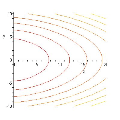
Figure 1: Level sets for the energy function (15) with $p=3/2$.

Indeed, we can compute $\mathcal{C}_{p}(S)$ for the slab using just the knowledge that a positive solution to (7) depends only on $x_{n}$. On the truncated domain $D_{R}$, we have

$$\int_{D_{R}}|\nabla u|^{2}dV=(2R)^{n-1}\int_{-1}^{1}(\partial_{x_{n}}u)^{2}dx_{n}=C_{1}R^{n-1},$$

while

$$\left(\int_{D_{R}}u^{p}dV\right)^{2/p}=(2R)^{\frac{2}{p}(n-1)}\left(\int_{-1}^{1}u^{p}(x_{n})dx_{n}\right)^{2/p}=C_{2}R^{\frac{2}{p}(n-1)}.$$

Taking a ratio we see that $\Phi_{p}(u)=\mathcal{O}(R^{(n-1)(1-\frac{2}{p})})$, and so

$$\mathcal{C}_{p}(S)=\left\{\begin{array}[]{cc}0&1\leq p<2\\ \frac{\pi^{2}}{4}&p=2\\ \infty&p>2,\end{array}\right.$$

where in the $p=2$ case we have listed the (well-known) value of the first Dirichlet eigenvalue of the Laplacian of a slab of width $2$.

Remark 3.

Notice that the solution for a slab does not depend on dimension at all.

Next we examine the case of the ball. By a moving planes argument [GNN], any positive solution to (7) is radial.

We treat the cases $n=2$ and $n\geq 3$ separately. First consider the unit disc in the plane. A radial solution $u$ will satisfy the ODE

$$u^{\prime\prime}+\frac{1}{r}u^{\prime}+\Lambda u^{p-1}=0,\qquad u(1)=0.$$

Change variables by $t=-\log(r)$ and let $v(t)=u(e^{-t})$ to get the boundary value problem

$$e^{2t}\ddot{v}+\Lambda v^{p-1}=0,\qquad v(0)=0,$$ (16)

where the $\lim_{t\rightarrow\infty}v(t)$ exists and is a positive number. Here we have used a dot to denote differentiation with respect to $t$ and a dash to denote differentiation with respect to $r$.

In dimension $n\geq 3$ a radial solution will satisfy the ODE

$$u^{\prime\prime}+\frac{n-1}{r}u^{\prime}+\Lambda u^{p-1}=0,\qquad u(1)=0.$$

We do a similar change of variables, but this time rescale $v$ by a radial factor, letting $u=e^{-kt}v(t)$, where again $t=-\log(r)$. Again, we will use a dot to denote differentiation with respect to $t$ and a dash to denote differentiation with respect to $r$. Under this change of variables, the ODE becomes

$$e^{(2-k)t}(\ddot{v}+(n+2k-2)\dot{v}+k(n+k-2)v)+\Lambda e^{-k(p-1)t}v^{p-1}=0,\qquad v(0)=0,$$ (17)

where $\lim_{t\rightarrow\infty}e^{-kt}v(t)$ exists and is a positive number. We can eliminate the $\dot{v}$ term by choosing $k=\frac{2-n}{2}$, and so (17) is now

$$e^{\frac{(n+2)t}{2}}\left(\ddot{v}-\left(\frac{n-2}{2}\right)^{2}v\right)+\Lambda e^{\frac{(n-2)(p-1)t}{2}}v^{p-1}=0.$$ (18)

In the critical case of $p=\frac{2n}{n-2}$, the exponential terms coincide, and we obtain the familiar differential equation

$$\ddot{v}-\left(\frac{n-2}{2}\right)^{2}v+\Lambda v^{\frac{n+2}{n-2}}=0,$$

which has the energy function

$$E=\frac{1}{2}(\dot{v})^{2}-\frac{(n-2)^{2}}{2}v^{2}+\frac{(n-2)\Lambda}{2n}v^{\frac{2n}{n-2}}.$$ (19)

Solutions will lie on level sets of $E$ in the phase plane; see the discussion in [Sc] for more details. We sketch some level sets of the energy function (19) below.

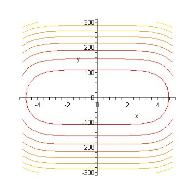
Figure 2: Level sets for the energy function (19) with $n=3$ and $p=6$.

4 Comparisons

In this section we prove some basic comparison principles for minimizers of $\Phi_{p}$. The first such comparison is domain monotonicity.

Proposition 8.

If $D_{1}\subset D_{2}\subset\mathbb{R}^{n}$ are bounded domains and $p\geq 1$ then $\mathcal{C}_{p}(D_{1})\geq\mathcal{C}_{p}(D_{2})$.

Proof.

This follows from the fact that $L^{p}(D_{1})\cap W^{1,2}_{0}(D_{1})\subset L^{p}(D_{2})\cap W^{1,2}_{0}(D_{2})$. ∎

Next we fix the domain $D$ and vary $p$.

Proposition 9.

Fix a smooth, bounded domain $D\subset\mathbb{R}^{n}$, and let $\mathcal{C}_{p}(D)$ be given by (5) for $p\geq 1$. Then the function $p\mapsto\mathcal{C}_{p}(D)$ is continuous.

Proof.

Again, we use the fact that $C^{\infty}_{0}(D)$ is dense in $L^{p}(D)\cap W^{1,2}_{0}(D)$ and take $u$ to be a smooth function. In this case, the function

$$p\mapsto\left(\int_{D}u^{p}dV\right)^{2/p}$$

is smooth, so $\Phi_{p}(u)$ is a smooth function of $p$ for fixed $u\in C^{\infty}_{0}(D)$. The proposition follows from the definition of $\mathcal{C}_{p}$. ∎

Our main result in this section is Theorem 3, which reads

$$V^{2/p}\mathcal{C}_{p}(D)>V^{2/q}\lambda_{q}(D)$$

for $1\leq p<q$, where $V=\operatorname{Vol}(D)$.

Proof.

Recall that $C^{\infty}_{0}(D)$ is dense in both $L^{p}(D)\cap W^{1,2}_{0}(D)$ and $L^{q}(D)\cap W^{1,2}_{0}(D)$, so for the purposes of our comparison it will suffice to take $u\in C^{\infty}_{0}(D)$. In particular, $u\in L^{p}(D)\cap L^{q}(D)$. Use Hölder’s inequality on the functions $u^{p}$ and $1$, with exponents $q/p$ and $q/(q-p)$, to obtain

$$\left(\int_{D}u^{p}dV\right)^{2/p}\leq\left[V^{\frac{q-p}{q}}\left(\int_{D}(u^{p})^{q/p}dV\right)^{p/q}\right]^{2/p}=V^{\frac{2(q-p)}{qp}}\left(\int_{D}u^{q}dV\right)^{2/q}.$$

Then, by the variational character of $\mathcal{C}_{p}$ and $\mathcal{C}_{q}$, we have

$$\mathcal{C}_{p}(D)=\inf\left\{\frac{\int_{D}|\nabla u|^{2}dV}{\left(\int_{D}u^{p}dV\right)^{2/p}}\right\}\geq V^{\frac{2(p-q)}{pq}}\inf\left\{\frac{\int_{D}|\nabla u|^{2}dV}{\left(\int_{D}u^{q}dV\right)^{2/q}}\right\}=V^{\frac{2(p-q)}{pq}}\mathcal{C}_{q}(D),$$

which gives the desired inequality. Finally, we can only have equality in Hölder’s inequality if $u$ is constant, which (by the boundary conditions) would force $u$ to be identically zero. This is impossible, and the inequality above must be strict. ∎

In dimension two one may take the limit as $p\to\infty$, to obtain

$$\mathcal{C}_{\infty}(D)=\inf\left\{\frac{\int_{D}|\nabla u|^{2}dV}{\|u\|_{L^{\infty}(D)}^{2}}:u\in L^{\infty}(D)\cap W^{1,2}_{0}(D),u\not\equiv 0\right\}=\lim_{p\rightarrow\infty}\mathcal{C}_{p}(D).$$

By the monotonicty of $V^{2/p}\mathcal{C}_{p}(D)$, this limit exists and is finite. Taking the limit as $p\to\infty$ in the scaling law (12) with $n=2$ shows that $\mathcal{C}_{\infty}(rD)=\mathcal{C}_{\infty}(D)$ for each positive $r$. For a fixed domain $D$, one can find disks $r\mathbb{D}$ and $R\mathbb{D}$ such that $r\mathbb{D}\subseteq D\subseteq R\mathbb{D}$, so that $\mathcal{C}_{\infty}(R\mathbb{D})\leq\mathcal{C}_{\infty}(D)\leq\mathcal{C}_{\infty}(r\mathbb{D})$ by domain monotonicity. On the other hand, $\mathcal{C}_{\infty}(r\mathbb{D})=\mathcal{C}_{\infty}(R\mathbb{D})$ by scale invariance. We see that $\mathcal{C}_{\infty}(D)$ does not depend on the domain at all, and write $\mathcal{C}_{\infty}$ for its common value for all planar domains.

We close this section with a preliminary estimate for $\mathcal{C}_{\infty}$.

Proposition 10.

$\mathcal{C}_{\infty}\leq\pi$.

Proof.

We may take $D$ to be the disk of radius $1$ centered at $0$. For any positive $\delta<1$, define the radial function

$$u(r)=\left\{\begin{array}[]{cc}1,&r<\delta\\ \frac{1-r}{1-\delta},&\delta\leq r\leq 1\end{array}\right.$$

Then $\|u\|_{L^{\infty}(D)}=1$. Moreover,

$$\int_{D}|\nabla u|^{2}dV=2\pi\int_{\delta}^{1}\left(\frac{1}{\delta-1}\right)^{2}r\,dr=\pi\frac{1+\delta}{1-\delta}.$$

so that

$$\lim_{\delta\rightarrow 0^{+}}\left[\int_{D}|\nabla u|^{2}dV\right]=\pi.$$ ∎

5 Extremal domains

In this section we characterize the domains which are maxima or minima for $\mathcal{C}_{p}$ under various constraints. We begin with a proof of Theorem 4, that the ball uniquely minimizes $\mathcal{C}_{p}(D)$ among all domains with a fixed volume. The proof follows the standard proof of the Faber-Krahn inequality by symmetrization.

Proof.

Let $u$ be a test function for $\Phi_{p}$. Without loss of generality, we can take $u\in C^{\infty}_{0}(D)$ and let

$$m=\min_{x\in D}\{u(x)\},\qquad M=\max_{x\in D}\{u(x)\}.$$

For $m\leq t\leq M$ let $D_{t}=\{u>t\}$.

Now we define a comparison function $u_{*}:B\rightarrow[m,M]$ as follows. First let $B_{t}$ be the ball centered at the origin with $\operatorname{Vol}(B_{t})=\operatorname{Vol}(D_{t})$. Then let $u_{*}$ be the radially symmetric function such that $B_{t}=\{u_{*}>t\}$. By the co-area formula,

$$\int_{t}^{M}\int_{\partial D_{\tau}}\frac{dA}{|\nabla u|}d\tau=\operatorname{Vol}(D_{t})=\operatorname{Vol}(B_{t})=\int_{t}^{M}\int_{\partial B_{\tau}}\frac{dA}{|\nabla u_{*}|}d\tau.$$

Differentiating with respect to $t$ gives

$$\int_{\partial D_{t}}\frac{dA}{|\nabla u|}=\int_{\partial B_{t}}\frac{dA}{|\nabla u_{*}|}$$ (20)

for all $t$. Then

$$\int_{D}u^{p}dV = \int_{m}^{M}\int_{\partial D_{t}}\frac{u^{p}dA}{|\nabla u|}dt=\int_{m}^{M}t^{p}\int_{\partial D_{t}}\frac{dA}{|\nabla u|}dt$$ (21)

$$= \int_{m}^{M}t^{p}\int_{\partial B_{t}}\frac{dA}{|\nabla u_{*}|}dt=\int_{B}u_{*}^{p}dV.$$

Now, for $m\leq t\leq M$ let

$$\psi(t)=\int_{D_{t}}|\nabla u|^{2}dV,\qquad\psi_{*}(t)=\int_{B_{t}}|\nabla u_{*}|^{2}dV.$$

By the co-area formula

$$\psi^{\prime}=-\int_{\partial D_{t}}|\nabla u|dA,\qquad\psi_{*}^{\prime}=-\int_{\partial B_{t}}|\nabla u_{*}|dA.$$

We use the Cauchy-Schwarz inequality, the isoperimetric inequality, and the fact that the normal derivative of $u_{*}$ is constant on $\partial B_{t}$ to see

$$\left(\int_{\partial D_{t}}|\nabla u|\,dA\right)\left(\int_{\partial D_{t}}\frac{dA}{|\nabla u_{*}|}\right) \geq \left(\int_{\partial D_{t}}\,dA\right)^{2}=\left(\operatorname{Area}(\partial D_{t})\right)^{2}$$

$$\geq \left(\operatorname{Area}(\partial B_{t})\right)^{2}=\left(\int_{\partial B_{t}}|\nabla u_{*}|\,dA\right)\left(\int_{\partial B_{t}}\frac{dA}{|\nabla u_{*}|}\right).$$

We use equation (20) to cancel the common factor of

$$\int_{\partial D_{t}}\frac{dA}{|\nabla u|}=\int_{\partial B_{t}}\frac{dA}{|\nabla u_{*}|},$$

and so

$$-\psi^{\prime}=\int_{\partial D_{t}}|\nabla u|\,dA\geq\int_{\partial B_{t}}|\nabla u_{*}|\,dA=-\psi_{*}^{\prime}.$$

Integrating this last differential inequality and using $\psi(M)=0=\psi_{*}(M)$ we see that

$$\int_{D}|\nabla u|^{2}dV=\psi(0)\geq\psi_{*}(0)=\int_{B}|\nabla u_{*}|^{2}dV.$$

This inequality, combined with (21) and (5), give the desired inequality on the eigenvalues:

$$\mathcal{C}_{p}(D)\geq\mathcal{C}_{p}(B).$$

Moreover, equality of the eigenvalues forces all level sets $\partial D_{t}$ to be spheres centered at the origin. Also, the equality case of the Cauchy-Schwarz inequality forces $|\nabla u|$ to be constant on the level set $\partial D_{t}$. Thus $u$ must be radially symmetric, and so in this case $u=u_{*}$. ∎

Next we fix the inradius $R(D)$ of the domain rather than the volume, where $R(D)$ is the supremum radius of all balls contained in $D$.

Lemma 11.

Among all bounded domains $D\subset\mathbb{R}^{n}$ with a fixed inradius, the ball maximizes $\mathcal{C}_{p}$ for all $p\geq 1$.

Proof.

If the inradius of $D$ is $R$, then $D$ contains a ball of radius $r$ for each $r<R$. The result now follows from domain monotonicity. ∎

Proposition 12.

Let $p\geq 1$. Let $D$ be a smooth, convex domain $D\subset\mathbb{R}^{n}$ with inradius $R$. Let $u>0$ solve (7) on $D$ and let $u_{M}=\max\{u(x):x\in D\}$. Then

$$u_{M}^{2-p}\leq\frac{2\Lambda R^{2}}{pA_{p}^{2}},$$ (22)

where

$$A_{p}=\int_{0}^{1}\frac{dt}{\sqrt{1-t^{p}}}=\sqrt{\pi}\frac{\Gamma(1+\frac{1}{p})}{\Gamma(\frac{1}{2}+\frac{1}{p})}.$$

Moreover, (22) is an equality in the case of a slab.

Remark 4.

By the discussion in the introduction, the maximum $u_{M}$ is well-defined.

Hersch [Her, Théorème 8.1] proved $\lambda(D)\geq\pi^{2}/(4R^{2})$ for the fundamental frequency while Sperb [Sp] proved $u_{M}\leq R^{2}$ for the maximum value of the torsion function, in each case for a convex domain of inradius $R$. The estimate (22) is a common generalisation of these results. More refined results are known in the cases $p=1$ and $p=2$ (see [MH], for example).

Proof.

We follow Section 6.2.2 of [Sp]. The $P$-function

$$v(x)=|\nabla u(x)|^{2}+\frac{2\Lambda}{p}u^{p}(x),$$

introduced by Payne, assumes its maximum at the point where $u$ assumes its maximum. Thus

$$|\nabla u(x)|^{2}+\frac{2\Lambda}{p}u^{p}(x)\leq\frac{2\Lambda}{p}u_{M}^{p},$$

which we can rearrange to read

$$|\nabla u(x)|\leq\sqrt{\frac{2\Lambda}{p}}\sqrt{u_{M}^{p}-u^{p}(x)}.$$ (23)

Let $\delta_{D}(P)$ be the distance from the point $P$ where $u$ assumes its maximum to the boundary of $D$ and integrate (23) along a line segment which starts at $P$ and terminates at a point on $\partial D$ closest to $P$. Then

$$R(D)\geq\delta_{D}(P)\geq\sqrt{\frac{p}{2\Lambda}}u^{(2-p)/2}A_{p}\quad\text{where }A_{p}=\int_{0}^{1}\frac{dt}{\sqrt{1-t^{p}}}.$$

The inequality (22) follows. Moreover, if $D$ is a slab then (15) implies (23) is actually an equality, and so (22) is also an equality. ∎

6 Open questions

In this final section we collect a small sample of interesting, related questions.

In the present paper, we have restricted our attention to the minimizer of the the functional $\Phi_{p}$, which corresponds to the bottom of the spectrum of the eigenvalue equation

$$\Delta u+\lambda u^{p-1}=0.$$

This functional should have other critical points above the minimizer, which correspond to sign changing solutions of the boundary value problem (7). What can one say about these higher order eigenvalues? If $n\geq 3$ and $p<\frac{2n}{n-2}$ (or if $n=2$) is the spectrum discrete? Is there a sequence of eigenvalues $\lambda_{p,j}$, with $j=1,2,3,\dots$, such that

$$0<\lambda_{p,1}<\lambda_{p,2}\leq\lambda_{p,3}\leq\cdots\rightarrow\infty?$$

We return to the minimum $\mathcal{C}_{p}(D)=\inf\{\Phi_{p}(u)\}$. In dimension $n\geq 3$, does the limit of $\mathcal{C}_{p}(D)$ exist as $p\rightarrow\frac{2n}{n-2}$ from below? It would be nice to characterize the domains on which the limit exists, in terms of geometry. We showed in Proposition 9 that the eigenvalue $\mathcal{C}_{p}$ is a continuous function of $p$. Is the same true of the eigenfunction? We have shown that, in dimension two, $\lim_{p\to\infty}\mathcal{C}_{p}(D)=\mathcal{C}_{\infty}$ exists and is independent of the domain. Can the bound $\mathcal{C}_{\infty}\leq\pi$ be improved or is it sharp? We proved the inequality (22) is realized in the case of a slab. Are there any other domains for which (22) is an equality?

References

- [F] C. Faber. Beweiss, dass unter allen homogenen Membrane von gleicher Fläche und gleicher Spannung die kreisförmige die tiefsten Grundton gibt. Sitzungsber.–Bayer. Akad. Wiss., Math.–Phys. Munich. (1923), 169–172.
- [GNN] B. Gidas, W.-M. Ni, and L. Nirenberg. Symmetry and related properties via the maximum principle. Comm. Math. Phys. 68 (1979), 209–243.
- [GT] D. Gilbarg and N. Trudinger. Elliptic Partial Differential Equations of Second Order, Third Edition. Springer-Verlag (2001).
- [Her] J. Hersch. Sur la fréquence fondamentale d’une membrane vibrante: évaluations par défault et principe de maximum. Z. Angew. Math. Mech. 11 (1960), 387–413.
- [Kor] N. Korevaar. Convex solutions to nonlinear elliptic and parabolic boundary value problems. Indiana Univ. Math. J. 32 (1983), 603–614.
- [K] E. Krahn. Über eine von Rayleigh formulierte Minmaleigenschaft des Kreises. Math. Ann. 94 (1925), 97–100.
- [LP] J. Lee and T. Parker. The Yamabe problem. Bull. Amer. Math. Soc. 17 (1987), 37–91.
- [MH] P.J. Méndez-Hernández, Brascamp-Lieb-Luttinger inequalities for convex domains of finite inradius. Duke Math. J. 113 (2002), 93–131.
- [Poh] S. Pohozaev. Eigenfunctions of the equation . Soviet Math. Doklady 6 (1965), 1408–1411.
- [P] G. Pólya, Torsional rigidity, principal frequency, electrostatic capacity and symmetrization. Quarterly J. Applied Math., 6 (1948), 267–277.
- [PS] G. Pólya and G. Szegő. Isoperimetric Inequalities in Mathematical Physics. Princeton University Press (1951).
- [Sc] R. Schoen. Variation theory for the total scalar curvature functional for Riemannian metrics and related topics. in Topics in Calculus of Variations (Montecantini Terme, 1987), 120–154. Lecture Notes in Math. 1265, Springer-Verlag. (1989).
- [Sp] R. Sperb. Maximum principles and their applications. Academic Press, Inc. (1981).
- [Tr] N. Trudinger. Remarks concerning the conformal deformation of Riemannian structures on compact manifolds. Ann. Scuola Norm. Sup. Pisa 22 (1968), 265–274.