Marching toward the eigenvalues: The Canonical Function Method and the Schrödinger equation

Abstract

The Canonical Function Method (CFM) is a powerful accurate and fast method that solves the Schrödinger equation for the eigenvalues directly without having to evaluate the eigenfunctions. Its versatility allows to solve several types of problems and in this work it is applied to the solution of several 1D potential problems, the 3D Hydrogen atom and the Morse potential.

I Introduction

The Canonical Function Method (CFM) is a powerful means for solving the Schrödinger equation and getting the eigenvalue spectrum directly in a fast and precise manner without computing the eigenfunctions.

The CFM turns the two-point boundary value (TPBV) Schrödinger problem into an initial value problem and allows full and accurate determination of the spectrum. This is done by expressing the solution as a sum of two linearly independent functions (the Canonical Functions) with specific values at some arbitrary point belonging to the interval defined by the two boundaries. The integration proceeds simultaneously from this point toward the left and right boundaries evaluating at each step a corresponding ratio. It stops when the difference between the left and right ratios is below a given desired precision.

This work is relevant to students who have completed an undergraduate Quantum Mechanics course of the Merzbacher Merzbacher level or graduate students whose level corresponds to Landau and Lifshitz course Landau and are interested in the eigenvalue problem of Quantum Mechanics.

The CFM can handle a large variety of Quantum problem problems Tannous besides the eigenvalue problem making it an extremely versatile, fast and highly accurate. The evaluation of the Schrödinger operator spectrum is done without performing diagonalization, bypassing the evaluation of the eigenfunctions. This allows to preserve a high degree of numerical precision that is required in solving sensitive eigenvalue problems.

It also solves the Radial Schrödinger equation over the infinite interval $[0,\infty[$ , where singularities in the potential at both boundaries are encountered.

The CFM method is superior to many standard techniques that have been used to solve the Schrödinger equation such as Numerov Numerov or relaxation methods that are particularly tailored for solving TPBV problems (see the Physics Reports Review Tannous ).

It is worthwhile to point out that, numerically, the precision gained with the bypass of intermediate diagonalization operations is reminiscent of the Golub-Reinsch algorithm (see for instance ref. Recipes ) used for the singular value decomposition of arbitrary rectangular matrices.

This article is organised as follows: The next section is a description of the CFM in 1D with the appropriate boundary conditions (BC). Several 1D problems are treated: The Infinite depth potential well, the finite depth potential well, the Harmonic Oscillator problem, the Kronig-Penney potential and the double-well (symmetric and asymmetric) potentials. In section III the CFM is applied to the 3D Schrödinger equation specializing to the Radial Schrödinger equation problems and in particular to the Hydrogen atom and the Morse potential. Finally section IV bears our conclusions.

In the Appendix we provide information on the different systems of units used in Atomic physics and quantum mechanics.

II One-dimensional potential problems

The CFM approach is based on the direct calculation of the eigenvalues of the Schrödinger equation defined over an interval $[x_{1},x_{2}]$ with a set of BC defining the problem:

$$[-\frac{\hbar^{2}}{2m_{e}}\frac{d^{2}}{dx^{2}}+V(x)]\psi(x)=E\psi(x),\hskip 5.69054ptx_{1}\leq x\leq x_{2}$$ (1)

$m_{e}$ is the electron mass.

Starting from a point $x_{0}\in[x_{1},x_{2}]$ we express the solution as a superposition of two linearly independent functions $\alpha(E;x),\beta(E;x)$, (the Canonical Functions) depending on the energy $E$ and the abscissa $x$ such that:

$$y(x)=y(x_{0})\alpha(E;x)+y^{\prime}(x_{0})\beta(E;x)$$ (2)

The CFM is based on the extraction of the eigenvalues from the zeroes of the eigenvalue function $F(E)$ defined from the saturation of the left ($x\rightarrow x_{1}$) and right ($x\rightarrow x_{2}$) functions $l_{-}(E)$ and $l_{+}(E)$ given by the ratios of the canonical functions $\alpha(E;x)$ and $\beta(E;x)$ or their derivatives.

In the general case when either $y(x_{1})\neq 0$ or $y(x_{2})\neq 0$ we write:

$$y(x) =y(x_{0})\alpha(E;x)+y^{\prime}(x_{0})\beta(E;x)$$

$$y^{\prime}(x) =y(x_{0})\alpha^{\prime}(E;x)+y^{\prime}(x_{0})\beta^{\prime}(E;x)$$ (3)

The canonical functions satisfy the following conditions at the starting point $x_{0}$:

$$\alpha(E;x_{0})=1,\alpha^{\prime}(E;x_{0})=0,$$

$$\beta(E;x_{0})=0,\beta^{\prime}(E;x_{0})=1$$ (4)

Let us rewrite the system 3 at the two boundaries $x=x_{1}$ and $x=x_{2}$:

$$y(x_{1}) = y(x_{0})\alpha(E;x_{1})+y^{\prime}(x_{0})\beta(E;x_{1});$$

$$y^{\prime}(x_{1}) = y(x_{0})\alpha^{\prime}(E;x_{1})+y^{\prime}(x_{0})\beta^{\prime}(E;x_{1});$$

$$y(x_{2}) = y(x_{0})\alpha(E;x_{2})+y^{\prime}(x_{0})\beta(E;x_{2});$$

$$y^{\prime}(x_{2}) = y(x_{0})\alpha^{\prime}(E;x_{2})+y^{\prime}(x_{0})\beta^{\prime}(E;x_{2})$$ (5)

Extracting from above the left and right ratios defining the functions $l_{-}(E)$ and $l_{+}(E)$:

$$l_{-}(E)=\left[\frac{y^{\prime}(x_{0})}{y(x_{0})}\right]_{-}=\frac{\alpha(E;x_{1})y^{\prime}(x_{1})-\alpha^{\prime}(E;x_{1})y(x_{1})}{\beta^{\prime}(E;x_{1})y(x_{1})-\beta(E;x_{1})y^{\prime}(x_{1})};$$

$$l_{+}(E)=\left[\frac{y^{\prime}(x_{0})}{y(x_{0})}\right]_{+}=\frac{\alpha(E;x_{2})y^{\prime}(x_{2})-\alpha^{\prime}(E;x_{2})y(x_{2})}{\beta^{\prime}(E;x_{2})y(x_{2})-\beta(E;x_{2})y^{\prime}(x_{2})}$$

In order to tackle any problem with the CFM, a number of constraints should be explained and underlined in order to illustrate the methodology of getting properly the eigenvalue spectrum:

• Sensitivity, stability and accuracy:
  The spectrum depends on the zeroes of $F(E)=l_{+}(E)-l_{-}(E)$. This subtraction might lead in some cases to inaccuracies because the entire spectrum depends on the zeroes of $F(E)$. However, it holds the key of the stability of the CFM since two independent solution sets are generated at the point $x_{0}$ , with progress inwards to the left point $x_{1}$ and outwards toward the right point $x_{2}$. Since both sets contain, in general, linear combinations of the regular and the irregular solutions, by suitably combining them, the irregular solution is eliminated.

• $x_{0}$ issue and the number of eigenvalues:
  The number of eigenvalues depend strongly on $x_{0}$. Thus, it should be chosen such that a $\tan(E)$-like diagram for the energy function $F(E)$ is obtained. In the case we have a potential displaying a single minimum, $x_{0}$ should be close to the potential minimum.

• Behaviour of the canonical functions:
  The method being sensitive to convergence of the marching toward the left-right boundaries $x_{1},x_{2}$, one ought to look for similar behaviour in the canonical functions $\alpha(E;x)$ and $\beta(E;x)$ along with the limiting process $x\rightarrow x_{1}$ and $x\rightarrow x_{2}$ since it controls the ratio saturation.

• Overall aspect of the eigenvalue function:
  The eigenvalue function $F(E)=l_{+}(E)-l_{-}(E)$ should have a regular structure of the $\tan(E)$ type, that is almost periodic versus $\ln(E)$.

There are several types of BC from the eigenvalue function defined as the difference between left and right ratio functions:

$$F(E)=l_{+}(E)-l_{-}(E)=\left[\frac{y^{\prime}(x_{0})}{y(x_{0})}\right]_{+}-\left[\frac{y^{\prime}(x_{0})}{y(x_{0})}\right]_{-}$$ (7)

We consider, for illustration, the following four types of BC:

1. Null wavefunctions BC:
   The conditions $y(x_{1})=y(x_{2})=0$ yield:

   $$l_{-}(E)=\lim_{x\rightarrow x_{1}}-\frac{\alpha(E;x)}{\beta(E;x)};$$

   $$l_{+}(E)=\lim_{x\rightarrow x_{2}}-\frac{\alpha(E;x)}{\beta(E;x)}$$ (8)

2. Null wavefunction and its derivative BC:
   The conditions $y(x_{1})=y^{\prime}(x_{2})=0$ yield:

   $$l_{-}(E)=\lim_{x\rightarrow x_{1}}-\frac{\alpha(E;x)}{\beta(E;x)};$$

   $$l_{+}(E)=\lim_{x\rightarrow x_{2}}-\frac{\alpha^{\prime}(E;x)}{\beta^{\prime}(E;x)}$$ (9)

3. Null derivative and the wavefunction BC:
   The conditions $y^{\prime}(x_{1})=y(x_{2})=0$ yield:

   $$l_{-}(E)=\lim_{x\rightarrow x_{1}}-\frac{\alpha^{\prime}(E;x)}{\beta^{\prime}(E;x)};$$

   $$l_{+}(E)=\lim_{x\rightarrow x_{2}}-\frac{\alpha(E;x)}{\beta(E;x)}$$ (10)

4. Null derivatives BC:
   The conditions $y^{\prime}(x_{1})=y^{\prime}(x_{2})=0$ yield:

   $$l_{-}(E)=\lim_{x\rightarrow x_{1}}-\frac{\alpha^{\prime}(E;x)}{\beta^{\prime}(E;x)};$$

   $$l_{+}(E)=\lim_{x\rightarrow x_{2}}-\frac{\alpha^{\prime}(E;x)}{\beta^{\prime}(E;x)}$$ (11)

It is remarkable that the eigenvalue function $F(E)=l_{+}(E)-l_{-}(E)$ behaves in a very peculiar way close to the trigonometric $\tan(E)$ shape as displayed in Fig.  1. This will be explained in the next section.

II.1 The Infinitely deep square well

Let us apply the CFM to the infinite square well potential of width $a$ defined by:
$V(x)=0,\hskip 5.69054pt0<x<a,V(0)=\infty,V(a)=\infty$, meaning $x_{1}=0,x_{2}=a$.

Figure 1: Eigenvalue function versus energy displaying the first 25 eigenvalues of the Infinite square well. The vertical lines indicate the eigenvalue position. The eigenvalue function has an approximate $\tan(E)$ shape versus the energy $E$.

The Schrödinger equation writes:

$$-\frac{\hbar^{2}}{2m_{e}}\frac{d^{2}\psi(x)}{dx^{2}}=E\psi(x),\hskip 5.69054pt0<x<a$$ (12)

with BC: $\psi(0)=0,\psi(a)=0$. The exact eigenfunctions are hence given by $\psi_{n}(x)=\sqrt{\frac{2}{a}}\sin(\frac{n\pi x}{a}),n=1,2...$ yielding the exact eigenvalues as: $E_{n}=\frac{\hbar^{2}}{2m_{e}}{(\frac{n\pi}{a})}^{2}$ with $m_{e}$ the electron mass.
In order to apply, the CFM method, we first note that the solutions are odd or even over the interval $[0,a]$. Working on the half-interval $[0,\frac{a}{2}]$ we can start from any point $x_{0}$ and apply the general methodology albeit with a modification regarding the matching conditions at the middle interval point.

In the odd-mode case (null wavefunctions at both boundaries $x_{1}=0,x_{2}=\frac{a}{2}$):

$$l_{-}(E)=\lim_{x\rightarrow 0}-\frac{\alpha(E;x)}{\beta(E;x)};$$

$$l_{+}(E)=\lim_{x\rightarrow\frac{a}{2}}-\frac{\alpha(E;x)}{\beta(E;x)};$$

$$F_{o}(E)=l_{+}(E)-l_{-}(E)$$ (13)

whereas in the even-mode case we have (null wavefunction at left boundary $x_{1}=0$, null derivative at right boundary $x_{2}=\frac{a}{2}$):

$$l_{-}(E)=\lim_{x\rightarrow 0}-\frac{\alpha(E;x)}{\beta(E;x)};$$

$$l_{+}(E)=\lim_{x\rightarrow\frac{a}{2}}-\frac{\alpha^{\prime}(E;x)}{\beta^{\prime}(E;x)};$$

$$F_{e}(E)=l_{+}(E)-l_{-}(E)$$ (14)

Solving successively $F_{o}(E)$ and $F_{e}(E)$ for the odd modes and the even modes, we get Table 1.

Index	CFM	Exact
1	1.6006952(-3)	1.6000001(-3)
3	1.4406255(-2)	1.4400001(-2)
5	4.0017359(-2)	4.0000003(-2)
7	7.8434058(-2)	7.8400001(-2)
9	0.1296562	0.1296000
11	0.1936839	0.1936000
13	0.2705172	0.2704000
15	0.3601561	0.3600000
17	0.4626004	0.4624000
19	0.5778504	0.5776000
21	0.7059059	0.7056000
23	0.8467670	0.8464000
25	1.000433	1.000000
2	6.4027691(-3)	6.4000003(-3)
4	2.5611134(-2)	2.5600001(-2)
6	5.7624962(-2)	5.7600003(-2)
8	0.1024444	0.1024000
10	0.1600693	0.1600000
12	0.2304998	0.2304000
14	0.3137361	0.3136000
16	0.4097775	0.4096000
18	0.5186247	0.5184000
20	0.6402774	0.6400000
22	0.7747357	0.7744000
24	0.9219995	0.9216000

Table 1: First twenty-five odd and even quantum levels of the infinite square well potential given by the CFM along with exact results. The well width $a$ is chosen in a way such that the eigenvalue is 1 when the level index is 25. The numbers in parenthesis represent a power of 10. All eigenvalues are in Atomic units (see Appendix).

II.2 The Finite depth square well

The finite depth square well potential of width $a$ is defined by: $V(x)=0,\hskip 5.69054pt\mbox{for}\hskip 5.69054pt0<x<a;\hskip 5.69054ptV(x)=V_{0};\hskip 5.69054pt\mbox{for}\hskip 5.69054ptx\geq a\hskip 5.69054pt\mbox{or}\hskip 5.69054ptx\leq 0$.

As in the Infinite depth case, the potential is symmetric with respect to the well center $\frac{a}{2}$, implying that we have odd and even modes. Therefore we take $x_{1}=-\infty,x_{2}=\frac{a}{2}$ which means that we march to the left through the potential step until we observe the nulling of the wavefunction, whereas the marching to the right results at half the potential well width $a$ in odd or even modes. More explicitly:

In the odd-mode case (null wavefunctions at both boundaries $x_{1}=-\infty,x_{2}=\frac{a}{2}$):

$$l_{-}(E)=\lim_{x\rightarrow-\infty}-\frac{\alpha(E;x)}{\beta(E;x)};$$

$$l_{+}(E)=\lim_{x\rightarrow\frac{a}{2}}-\frac{\alpha(E;x)}{\beta(E;x)};$$

$$F_{o}(E)=l_{+}(E)-l_{-}(E)$$ (15)

whereas in the even-mode case we have (null wavefunction at left boundary $x_{1}=-\infty$, null derivative at right boundary $x_{2}=\frac{a}{2}$):

$$l_{-}(E)=\lim_{x\rightarrow-\infty}-\frac{\alpha(E;x)}{\beta(E;x)};$$

$$l_{+}(E)=\lim_{x\rightarrow\frac{a}{2}}-\frac{\alpha^{\prime}(E;x)}{\beta^{\prime}(E;x)};$$

$$F_{e}(E)=l_{+}(E)-l_{-}(E)$$ (16)

Solving successively $F_{o}(E)$ and $F_{e}(E)$ for the odd modes and the even modes, we get the following table 2.

Index	CFM	Exact
1	1.6482281(-3)	1.6475233(-3)
3	1.4832322(-2)	1.4826014(-2)
5	4.1191306(-2)	4.1173782(-2)
7	8.0705732(-2)	8.0671579(-2)
9	0.1333447	0.1332882
11	0.1990615	0.1989772
13	0.2777881	0.2776708
15	0.3694246	0.3692691
17	0.4738183	0.4736193
19	0.5907167	0.5904695
21	0.7196453	0.7193471
23	0.8594448	0.8590948
2	6.5926472(-3)	6.5898113(-3)
4	2.6365897(-2)	2.6354689(-2)
6	5.9305709(-2)	5.9280563(-2)
8	0.1053872	0.1053425
10	0.1645720	0.1645023
12	0.2368039	0.2367037
14	0.3220005	0.3218648
16	0.4200394	0.4198628
18	0.5307267	0.5305039
20	0.6537226	0.6534503
22	0.7883219	0.7879974
24	0.9322464	0.9318770

Table 2: First 24 odd and even quantum levels of the finite depth square well potential given by the CFM along with exact results. The numbers in parenthesis represent a power of 10. The barrier height $V_{0}=1$ and all eigenvalues are in Atomic units (see Appendix).

Figure 2: Eigenvalue function versus energy displaying the first 15 eigenvalues of the finite square well. The vertical lines indicate the eigenvalue position. The eigenvalue function has an approximate $\tan(E)$ shape versus the energy $E$.

The exact eigenvalues $E_{n}=\frac{\hbar^{2}k_{n}^{2}}{2m}$, drawn from Landau-Lifshitz book Landau are given by the solutions $k_{n}\hskip 5.69054pt(n=1,2...)$ of the transcendental equation:

$$\sin^{-1}\frac{\hbar k_{n}}{\sqrt{2mV_{0}}}=\frac{1}{2}(n\pi-k_{n}a);\hskip 5.69054pt0\leq k_{n}\leq\sqrt{\frac{2mV_{0}}{\hbar^{2}}}$$ (17)

The number of levels gives us $a$ the well width in the following way: since the $\sin^{-1}$ term is bounded by $\frac{\pi}{2}$, the largest level index $n_{max}$ is given by $n_{max}=1+\frac{a}{\pi}\sqrt{\frac{2mV_{0}}{\hbar^{2}}}$, hence $a=\frac{\pi\hbar(n_{max}-1)}{\sqrt{2mV_{0}}}$.

II.3 The harmonic oscillator

The harmonic oscillator potential defined by: $V(x)=\frac{1}{2}kx^{2}$ is symmetric with respect to the origin $x=0$ implying as before that the solutions are given by odd and even parity modes. The boundaries for this problem are: $x_{1}=-\infty,x_{2}=0$.

In the odd-mode case (null wavefunctions at both boundaries $x_{1}=-\infty,x_{2}=0$):

$$l_{-}(E)=\lim_{x\rightarrow-\infty}-\frac{\alpha(E;x)}{\beta(E;x)};$$

$$l_{+}(E)=\lim_{x\rightarrow 0}-\frac{\alpha(E;x)}{\beta(E;x)};$$

$$F_{o}(E)=l_{+}(E)-l_{-}(E)$$ (18)

whereas in the even-mode case we have (null wavefunction at left boundary $x_{1}=-\infty$, null derivative at right boundary $x_{2}=0$):

$$l_{-}(E)=\lim_{x\rightarrow-\infty}-\frac{\alpha(E;x)}{\beta(E;x)};$$

$$l_{+}(E)=\lim_{x\rightarrow 0}-\frac{\alpha^{\prime}(E;x)}{\beta^{\prime}(E;x)};$$

$$F_{e}(E)=l_{+}(E)-l_{-}(E)$$ (19)

Solving successively $F_{o}(E)$ and $F_{e}(E)$ for the odd modes and the even modes, we get the following table 3.

Index	CFM	Exact
1	5.8842082(-2)	5.8823533(-2)
3	0.1372950	0.1372549
5	0.2157480	0.2156863
7	0.2941877	0.2941177
9	0.3726121	0.3725490
11	0.4510336	0.4509804
13	0.5294515	0.5294118
15	0.6078746	0.6078432
17	0.6863770	0.6862745
19	0.7654451	0.7647059
21	0.8468009	0.8431373
23	0.9335056	0.9215686
25	1.028182	1.000000
0	1.9617772(-2)	1.9607844(-2)
2	9.8067097(-2)	9.8039217(-2)
4	0.1765225	0.1764706
6	0.2549707	0.2549020
8	0.3334008	0.3333333
10	0.4118234	0.4117647
12	0.4902429	0.4901961
14	0.5686612	0.5686275
16	0.6471026	0.6470588
18	0.7257724	0.7254902
20	0.8056628	0.8039216
22	0.8892854	0.8823529
24	0.9797482	0.9607844

Table 3: Ground state (zero index) and first twenty-five odd and even excited states of the harmonic oscillator potential given by the CFM along with exact results. The numbers in parenthesis represent a power of 10. The oscillator elastic constant was chosen such that level 25 had value 1 in Atomic units. All eigenvalues are in Atomic units (see Appendix).

Figure 3: Eigenvalue function versus energy displaying the first 26 eigenvalues of the harmonic oscillator potential. The vertical lines indicate the eigenvalue position. The eigenvalue function has an approximate $\tan(E)$ shape versus the energy $E$.

The exact eigenvalues $E_{n}=\hbar\omega_{0}(n+\frac{1}{2})$ Landau allow us to pick the energy of the highest level as 1 (in Atomic units) from which we select the value of $\omega_{0}=\sqrt{\frac{k}{m}}$ and hence the elastic constant $k$.

II.4 Periodic potential: The Kronig-Penney problem

The Kronig-Penney potential is often used in the description of the electronic properties of crystals. It is based on a piecewise constant potential (see fig. 4) for which we can apply the same methodology of marching to the left and to the right and comparing corresponding ratios in order to get the eigenvalues. The latter are now dispersive which means they depend on a wavevector reflecting the translational symmetry of the system (Bloch theorem). The CFM must be extended to the complex case since previously all the wavefunctions we use and derive were real. It is straightforward to extend the marching method as well to the complex wavefunction case as explained below.

Figure 4: Periodic piecewise constant potential $V(x)$ displaying alternating regions of $V=0$ and $V=V_{0}$ with periodicity $a+b$. The energy bands are obtained for $E<V_{0}$. In the case we let $V_{0}\rightarrow\infty$ and $b\rightarrow 0$ the barriers become delta functions sitting on a periodic lattice with parameter $a$.

Defining a unitcell with extreme boundaries $-b$ and $a$ we write the general CFM definitions in the complex case:

$$y(-b) = y(x_{0})\alpha(E;-b)+y^{\prime}(x_{0})\beta(E;-b)$$

$$y^{\prime}(-b) = y(x_{0})\alpha^{\prime}(E;-b)+y^{\prime}(x_{0})\beta^{\prime}(E;-b)$$

$$y(a) = y(x_{0})\alpha(E;a)+y^{\prime}(x_{0})\beta(E;a)$$

$$y^{\prime}(a) = y(x_{0})\alpha^{\prime}(E;a)+y^{\prime}(x_{0})\beta^{\prime}(E;a)$$ (20)

The energy $E$ is considered as smaller than $V_{0}$. Using Bloch theorem Kittel , in the above equations:

$$y(a)=y(-b)\exp[ik(a+b)],y^{\prime}(a)=y^{\prime}(-b)\exp[ik(a+b)],$$ (21)

we get the complex ratio functions:

$$l_{-}(E)=\left[\frac{y^{\prime}(x_{0})}{y(x_{0})}\right]_{-}=\frac{\gamma\alpha(E;-b)-\alpha(E;a)}{\beta(E;a)-\gamma\beta(E;-b)};$$

$$l_{+}(E)=\left[\frac{y^{\prime}(x_{0})}{y(x_{0})}\right]_{+}=\frac{\gamma\alpha^{\prime}(E;-b)-\alpha^{\prime}(E;a)}{\beta^{\prime}(E;a)-\gamma\beta^{\prime}(E;-b)};$$

$$F(E)=l_{+}(E)-l_{-}(E)$$ (22)

where $\gamma=\exp[ik(a+b)]$. This yields the dispersion relation for the energy eigenvalue $\epsilon_{n}(k)$ with $n$ the band index:

$$[\gamma\alpha(E;-b)-\alpha(E;a)][\beta^{\prime}(E;a)-\gamma\beta^{\prime}(E;-b)]-$$

$$\hskip 14.22636pt[\beta(E;a)-\gamma\beta(E;-b)][\gamma\alpha^{\prime}(E;-b)-\alpha^{\prime}(E;a)]=0$$ (23)

We compare the above to the standard dispersion relation Kittel :

$$\frac{Q^{2}-\kappa^{2}}{2Q\kappa}\sinh(Qb)\sin(\kappa a)+\cosh(Qb)\cos\kappa a=\cos k(a+b)$$ (24)

where $Q$ is defined as the (pure imaginary) wavevector inside the potential barrier. Recall that the energy $E<V_{0}$ hence the wavefunction within the barrier is of the form $\exp(\pm Qx)$, i.e. when $V(x)=V_{0}$, $V_{0}=~{}\frac{\hbar^{2}Q^{2}}{2m_{e}}~{}+~{}\frac{\hbar^{2}\kappa^{2}}{2m_{e}}$ whereas $\kappa$ is the real free wavevector outside the barrier i.e. when $V(x)=0$ the wavefunction is of the form $\exp(\pm i\kappa x)$).

When we let $V_{0}\rightarrow\infty$ and $b\rightarrow 0$ such that $V_{0}b$ remains finite, the piecewise constant potential $V(x)$ is transformed into a periodic array of $\delta$ functions $g\delta(x-na)$ with lattice parameter $a$. $g$ is the strength of the delta function potential and $n\in Z$ a relative integer.

We can formally write the potential as:

$$V(x)=\sum_{n=-\infty}^{n=+\infty}g\delta(x-na)$$ (25)

and consider a single interval extending over the unit cell with boundaries $x_{1}=0$ and $x_{2}=a$. Since at the left boundary $x_{1}=0$ we have a $\delta$ function potential, standard quantum mechanics Merzbacher tell us that the wavefunction derivative $y^{\prime}(x)$ jumps across the $\delta$ function potential, such that:

$$y^{\prime}(0^{+})-y^{\prime}(0^{-})=g\frac{2m_{e}}{\hbar^{2}}y(0)$$ (26)

Bloch theorem Kittel transforms this equation into:

$$y^{\prime}(0^{+})-y^{\prime}(a^{-})\exp(-ika)=g\frac{2m_{e}}{\hbar^{2}}y(0)$$ (27)

The left ratio (complex) is thus obtained as:

$$l_{-}(E)=\frac{y^{\prime}(x_{0})}{y(x_{0})}=$$

$$\frac{-\alpha^{\prime}(E;0)+\alpha^{\prime}(E;a)\exp(-ika)+g\frac{2m_{e}}{\hbar^{2}}\alpha(E;0)}{\beta^{\prime}(E;0)-\beta^{\prime}(E;a)\exp(-ika)-g\frac{2m_{e}}{\hbar^{2}}\beta(E;0)}$$ (28)

The right ratio is determined from Bloch theorem linking the right boundary $x_{2}=a$ to the left boundary $x_{1}=0$: $y(a)=y(0)\exp(ika)$:

$$l_{+}(E)=\frac{y^{\prime}(x_{0})}{y(x_{0})}=\frac{\alpha(E;a)-\exp(ika)\alpha(E;0)}{\exp(ika)\beta(E;0)-\beta(E;a)}$$ (29)

The dispersion relation is obtained as before from the zeroes of:

$$F(E)=l_{+}(E)-l_{-}(E)=\frac{\alpha(E;a)-\exp(ika)\alpha(E;0)}{\exp(ika)\beta(E;0)-\beta(E;a)}$$

$$-\frac{g\frac{2m_{e}}{\hbar^{2}}-\alpha^{\prime}(E;0)+\alpha^{\prime}(E;a)\exp(-ika)\alpha(E;0)}{\beta^{\prime}(E;0)-\beta^{\prime}(E;a)\exp(-ika)-g\frac{2m_{e}}{\hbar^{2}}\beta(E;0)}$$ (30)

Indeed, the dispersion relation Kittel obtained from the limiting process $V_{0}\rightarrow\infty$ and $b\rightarrow 0$ is Kittel :

$$\frac{Q^{2}b}{2\kappa}\sin(\kappa a)+\cos\kappa a=\cos ka$$ (31)

can be straightforwardly obtained from the derivative jump condition (eq. 27) and Bloch theorem $y(a)=y(0)\exp(ika)$. Starting with the wave function $y(x)=A\exp(i\kappa x)+B\exp(-i\kappa x)$, defined over the unit cell $x\in]0,a[$ and using both aforementioned conditions yields the dispersion relation:

$$\frac{m_{e}g}{\kappa\hbar^{2}}\sin(\kappa a)+\cos\kappa a=\cos ka$$ (32)

Comparing both dispersion relations yields finally the value of the strength of the $\delta$ function potential as $g=\frac{Q^{2}b\hbar^{2}}{2m_{e}}$.

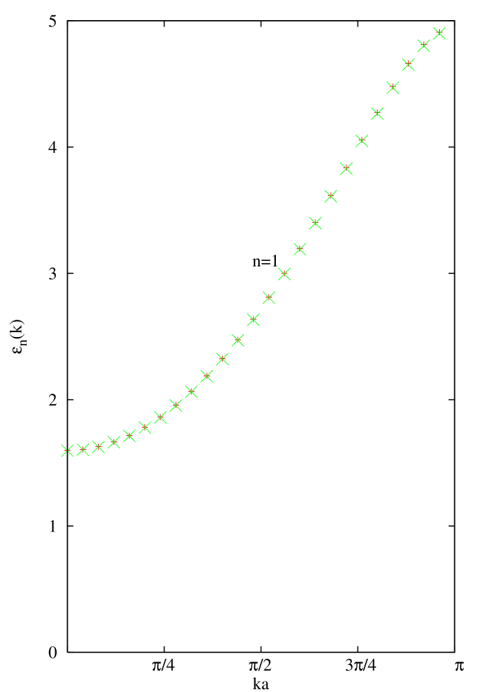
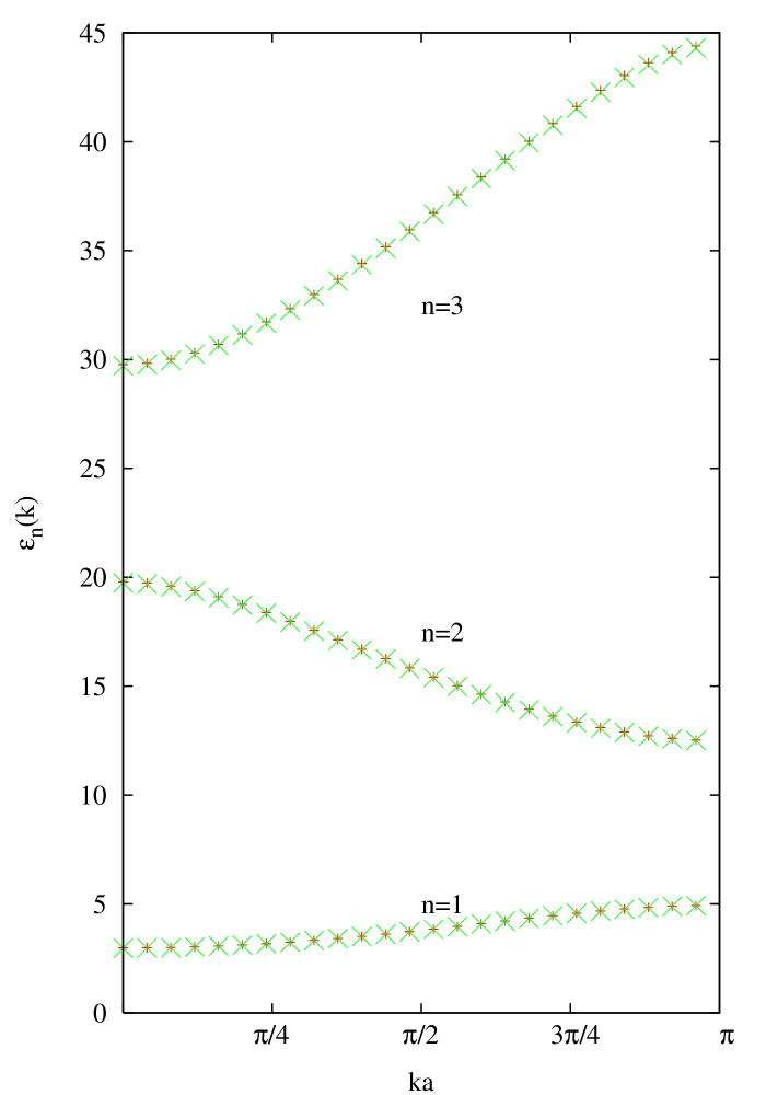
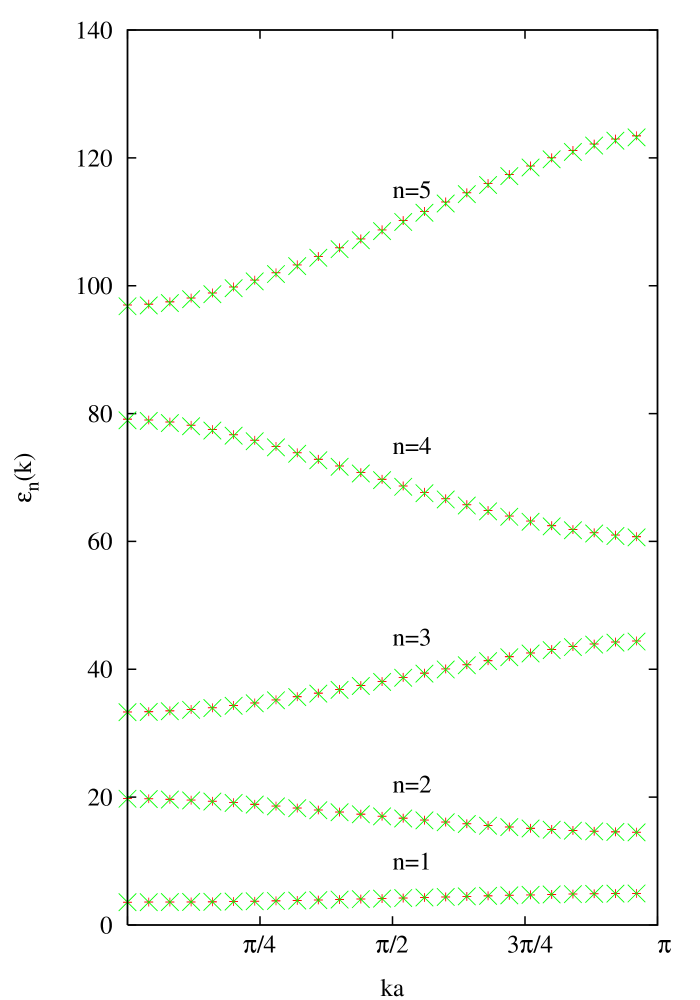
(a)	(b)	(c)

Figure 5: (Color on line) Exact bands (in green or ”$\times$”) for the Kronig-Penney model and comparison with the CFM bands (in red or ”+”) obtained from the dispersion relation obtained from eq. 30 and 28. (a) is for a single band, (b) and (c) are for 3 and 5 bands respectively with $a=2.22,6.66,11.12$ Atomic units. In all cases, the value of $x_{0}$ is 1 and the strength of the potential $g=1$ in Atomic units.

In figure 5, exact bands are compared to the CFM bands. The lattice parameter in each case is determined from the number of bands $n_{B}$ we want to calculate according to the formula: $a=\frac{n_{B}\pi\hbar}{\sqrt{2m_{e}}}$ since the largest wavenumber is $k_{max}=\frac{n_{B}\pi}{a}$ and we select the largest energy $E_{max}=\frac{\hbar^{2}k^{2}}{2m_{e}}$ as 1. This is why we use $a=2.22,6.66,11.12$ Atomic units for the $n_{B}=1,3,5$ respective number of bands. It is remarkable to observe how the CFM results lie exactly on top of the exact results. The starting value $x_{0}$ is chosen in a way such that we get the right number of bands $n_{band}$. Spurious bands might appear due to a bad starting value $x_{0}$ because the nature of the CFM dispersion relation 30 differs with respect to the dispersion relations eq. 31 and eq.32. The latter eq.32 allow the exact determination of the free wavevector $\kappa$ from a given Bloch wavevector $k$ and the exact band energy is obtained from $E=\frac{\hbar^{2}\kappa^{2}}{2m_{e}}$. In sharp contrast, the CFM dispersion relation 30 yields directly the band energy without going through the determination of an intermediate wavevector $\kappa$.

II.5 Double well potential over an infinite interval

Double-minimum Potential Well (DPW) problems defined over the semi-infinite interval $[0,\infty[$ are interesting to solve as they arise in many areas of Atomic, Molecular and even Solid State physics. When two-dimensional electron layers (such as in heterostructures involving semiconductors) are placed in perpendicular electric and magnetic fields, a potential well with two minima, for electronic motion normal to the surface, arises.

A DPW can be symmetric or asymmetric and one has to adapt in each case the appropriate BC imposed by the CFM.

A symmetric DPW is the Double Gaussian potential investigated by Hamilton and Light Ham given by:

$$V(x)=-D[\exp(-\Omega{(x-r_{a})}^{2})+\exp(-\Omega{(x+r_{a})}^{2})]$$

The values of the parameters: $D,\Omega,r_{a}$ are respectively: 12.0,0.1,5.0 in standard atomic units (see Appendix) such that $\hbar=1,m_{e}=1$.

An elaborate method used by Hamilton and Light Ham based on Distributed Gaussian Basis sets borrowed from Quantum Chemistry Techniques gives the eigenvalues listed in table 4. The CFM results for all the 24 levels in table 4 proves once again that it is able to find all levels with speed and accuracy from a simple marching approach.

Index	CFM	Hamilton and Light
1	-11.250 421 409	-11.245 199 313
3	-9.779 225 834	-9.773 496 902
5	-8.387 719 137	-8.381 307 491
7	-7.079 412 929	-7.072 038 846
9	-5.858 811 221	-5.849 940 0
11	-4.732 171 001	-4.720 509 6
13	-3.709 113 861	-3.690 475 6
15	-2.801 628 760	-2.763 219 7
17	-2.000 566 637	-1.924 577
19	-1.255 332 005	-1.149 254
21	-0.561 216 170	-0.457 88
23	-0.045 810 537	-0.003 41
0	-11.250 418 469	-11.245 199 313
2	-9.779 202 594	-9.773 496 902
4	-8.387 701 732	-8.381 307 510
6	-7.079 415 041	-7.072 039 562
8	-5.858 805 474	-5.849 958 02
10	-4.732 231 858	-4.720 829 36
12	-3.709 907 559	-3.694 518 38
14	-2.807 436 691	-2.798 251 92
16	-2.022 064 904	-2.089 661 3
18	-1.293 090 067	-1.462 202 9
20	-0.601 483 056	-0.771 081
22	-0.067 153 689	-0.177 181

Table 4: Computed odd and even eigenvalues for the symmetric double Gaussian well potential. The numbers at left are the levels computed with the CFM; on the right the levels obtained by Hamilton and Light Ham . Note the deterioration of accuracy of the Hamilton and Light results as the index increases because of the approach of the continuum.

The asymmetric DWP introduced by Johnson consists of the sum of a Morse (see next section) and a Gaussian potentials such that:

$$V(x)=D{[1-\exp(-B(x-r_{a}))]}^{2}+A\exp{(-C(x-r_{b})}^{2})$$

The values of the parameters $A,B,C,D,r_{a},r_{b}$ are (following Johnson Johnson ) in (cm^-1, Å  system of units) are: 10⁴ cm^-1, 1.54 Å^-1, 200.0 Å^-2, 31250.0 cm^-1, 1.5 Å, 1.6 Å  respectively.

Eigenvalues for the asymmetric double minimum potential problem are given in table 5 and a comparison between Johnson’s Johnson results and the CFM are displayed below.

Index	Johnson	CFM
0	1302.500	1302.498 972
1	3205.307	3205.303 782
2	4227.339	4227.336 543
3	5144.251	5144.243 754
4	6064.241	6064.225 881
5	7092.679	7092.664 815
6	7614.622	7614.603 506
7	8911.545	8911.513 342
8	9095.696	9095.679 497
9	10208.350	10208.318 142
10	10869.289	10869.255 077
11	11482.475	11482.457 956
12	12353.799	12353.766 422
13	12972.473	12972.453 117
14	13690.455	13690.436 602
15	14435.350	14435.321 044

Table 5: Eigenvalues in cm^-1 of the Johnson asymmetric DWP consisting of the sum of a Morse and a Gaussian potentials $V(r)=D{[1-\exp(-B(x-r_{a}))]}^{2}+A\exp{(-C(x-r_{b})}^{2})$. with $A$= 10⁴ cm^-1, $B$= 1.54 Å^-1, $C$= 200.0 Å^-2, $D$= 31250.0 cm^-1, and $r_{a}$ = 1.5 Å, $r_{b}$= 1.6 Å. Johnson Johnson results are compared to the CFM.

III The Canonical Function Method and the 3D Radial Schrödinger Equation

After having discussed the CFM in the 1D case, we move on to the treatment of the Radial Schrödinger Equation (RSE). The mathematical difficulty of the RSE lies in the fact it is a singular boundary value problem (SBVP). problem. This stems from the boundary conditions over the infinite interval $[0,\infty[$ , with the double requirement of regularity near the origin ($r\sim 0$) where the potential is large and near infinity ($r\rightarrow\infty$) where the potential is very small. The CFM turns it into a regular initial value problem and allows the full determination of the spectrum of the Schrödinger operator bypassing the evaluation of the eigenfunctions.

The partial wave form of the RSE is written as:

$$-\frac{\hbar^{2}}{2\mu}{\frac{d^{2}R_{l}(E;r)}{dr^{2}}}+\left[{V(r)+\frac{\hbar^{2}}{2\mu}\frac{l(l+1)}{r^{2}}}\right]R_{l}(E;r)=$$

$$\hskip 85.35826ptER_{l}(E;r)$$ (33)

where $\mu$ is the reduced mass and $R_{l}(E;r)$ is the reduced probability amplitude for orbital angular momentum $l$ and eigenvalue $E$.

The BC are:

$$\lim_{r\rightarrow 0}R_{l}(r)=0;\lim_{r\rightarrow+\infty}R_{l}(r)=0$$ (34)

The CFM consists of writing the general solution $y(r)$ representing the probability amplitude $R_{l}(E;r)$ as a function of the radial distance $r$ in terms of two linearly independent basis functions $\alpha(E;r)$ and $\beta(E;r)$ for some energy $E$.
Generally, the RSE is rewritten in a system of units such that $\hbar=1,2\mu=1$ (see Appendix on units):

$$\frac{d^{2}y(r)}{dr^{2}}=\left[{V(r)+\frac{l(l+1)}{r^{2}}-E}\right]y(r)$$ (35)

At a selected distance $r_{0}$, a well defined set of initial conditions are satisfied by the canonical functions and their derivatives ie: $\alpha(E;r_{0})=1$ with $\alpha^{\prime}(E;r_{0})=0$ and $\beta(E;r_{0})=0$ with $\beta^{\prime}(E;r_{0})=1$. Thus we write as in the 1D case:

$$y(r)=y(r_{0})\alpha(E;r)+y^{\prime}(r_{0})\beta(E;r)$$ (36)

The method of solving the RSE is to proceed from $r_{0}$ simultaneously towards the origin ($r\rightarrow 0$) and towards infinity ($r\rightarrow\infty$).

When the integration is performed, the ratio of the $r$ dependent canonical functions is monitored until saturation with respect to $r$ is reached at both limits ($r\rightarrow 0$ and $r\rightarrow\infty$). The saturation of the $\frac{\alpha(E;r)}{\beta(E;r)}$ ratio with $r$ yields a position independent eigenvalue function $F(E)$:

$$F(E)=l_{+}(E)-l_{-}(E)=\left[\frac{y^{\prime}(r_{0})}{y(r_{0})}\right]_{+}-\left[\frac{y^{\prime}(r_{0})}{y(r_{0})}\right]_{-}$$ (37)

The $\tan(E)$ shape of $F(E)$ provides a deep insight into the physical significance of the CFM method. The latter transforms a SBVP from the open interval $[0,\infty[$ to a finite interval $[r_{left},r_{right}]$ defined by the saturation coordinates of the ratio functions. This means the CFM maps an arbitrary potential $V(r)$ onto the infinite square well problem in the finite interval $[r_{left},r_{right}]$ resulting in an eigenvalue function $F(E)$ with a $\tan(E)$ pattern as we saw in Section II (see also ref. Johnson ).

III.1 The Hydrogen atom spectrum

The Coulomb potential is a crucial case to test the accuracy and reliability of the CFM given by the Hydrogen atom problem.

The CFM results are shown in Table. 6 along with the exact analytical results and it is remarkable to notice that all digits (calculated by CFM and analytically) are rigorously same.

Index	CFM (Ry)	Exact (Ry)
1	-1.00000	-1.00000
2	-0.250000	-0.250000
3	-0.111111	-0.111111
4	-6.25000(-2)	-6.25000(-2)
5	-4.00000(-2)	-4.00000(-2)
6	-2.77778(-2)	-2.77778(-2)
7	-2.04082(-2)	-2.04082(-2)
8	-1.56250(-2)	-1.56250(-2)
9	-1.23457(-2)	-1.23457(-2)
10	-1.00000(-2)	-1.00000(-2)
11	-8.26446(-3)	-8.26446(-3)
12	-6.94444(-3)	-6.94444(-3)
13	-5.91716(-3)	-5.91716(-3)
14	-5.10204(-3)	-5.10204(-3)
15	-4.44445(-3)	-4.44445(-3)
16	-3.90625(-3)	-3.90625(-3)
17	-3.46021(-3)	-3.46021(-3)
18	-3.08642(-3)	-3.08642(-3)
19	-2.77008(-3)	-2.77008(-3)
20	-2.50000(-3)	-2.50000(-3)
21	-2.26757(-3)	-2.26757(-3)
22	-2.06612(-3)	-2.06612(-3)
23	-1.89036(-3)	-1.89036(-3)
24	-1.73611(-3)	-1.73611(-3)

Table 6: Energy levels of the Hydrogen atom. Middle column values are the CFM results whereas the last column values are the corresponding exact analytically obtained values. The numbers in parenthesis represent a power of 10.

III.2 The Morse potential

The classical Morse potential is the simplest model for the evaluation of cell vibrational spectra of diatomic molecules.

The Morse potential is given by:

$$V(r)=D{[1-\exp(-a\{r-r_{e}\})]}^{2}-D$$ (38)

with the values $D,a,r_{e}$ equal respectively to 188.4355, 0.711248, 1.9975 in atomic units (see Appendix). The analytic expression for the levels is:

$$E_{n}=-\frac{a^{2}\hbar^{2}}{2\mu}(\frac{\sqrt{2\mu D}}{a}-n-\frac{1}{2})^{2},$$ (39)

with max $n\leq\frac{\sqrt{2\mu D}}{a}-\frac{1}{2}$. Hence the number of levels is given by: $N=\frac{\sqrt{2\mu D}}{a}-\frac{1}{2}$.

Working with units such that $\hbar=1$ and $2\mu=1$, the Morse potential and the eigenvalue function $F(E)$ are displayed in fig.6 and fig. 7 respectively. Table 7 contains the levels calculated by CFM and compared to the analytical analytical results. As in all previous cases, the agreement is perfect and the full set of levels ($N=19$) are found as predicted analytically.

Figure 6: Morse potential $V(r)=D{[1-\exp(-a\{r-r_{e}\})]}^{2}-D$ with parameters $D=188.4355,a=0.711248,r_{e}=1.9975$.

Index	CFM	Exact
1	-178.798248	-178.798538
2	-160.282181	-160.283432
3	-142.778412	-142.78006
4	-126.287987	-126.288445
5	-110.807388	-110.808578
6	-96.3395233	-96.3404541
7	-82.8832169	-82.884079
8	-70.4389801	-70.4394531
9	-59.0056	-59.0065727
10	-48.5851288	-48.5854378
11	-39.1754532	-39.1760521
12	-30.77771	-30.7784157
13	-23.3919983	-23.3925247
14	-17.0183048	-17.018383
15	-11.6557436	-11.6559868
16	-7.3050122	-7.30533791
17	-3.9661877	-3.9664371
18	-1.6390723	-1.63928342
19	-0.3238727	-0.32387724

Table 7: Energy levels of the Morse potential $V(r)=D{[1-\exp(-a\{r-r_{e}\})]}^{2}-D$ with parameters $D=188.4355,a=0.711248,r_{e}=1.9975$. Middle column values are the CFM results whereas the last column values are the corresponding exact analytically obtained values. Units are such that $\hbar=1$ and $2\mu=1$.

Figure 7: Behavior of the eigenvalue function $F(E)$ with absolute value of energy on a semi-log scale for the Morse potential.

IV Conclusions

The CFM is a very powerful, fast and accurate method that is able to evaluate the eigenvalue spectrum without having to determine first or simultaneously the eigenfunctions.

The CFM has been tested succesfully in a variety of potentials Tannous and gives accurate results for bound and free states. The tunable accuracy of our method allows to evaluate eigenvalues close to the ground state as well as close to highly excited states near the continuum limit to a large number of digits without any extrapolation.

The CFM compares favorably with many different elaborate techniques based on expansion over basis functions (such as Gaussian Johnson , Quantum Chemistry inspired basis functions Ham ) or functional expansions (Numerov Numerov , High-order Taylor Raptis …). The CFM approach remains the same despite the wide variability of the mentioned problems.

The CFM method used gives the right number of all the levels and the variation of the eigenvalue function $F(E)$ definitely determines the total number of levels. Generally in order to avoid potential singularities, Taylor series expansion are made to a given order dictated by the required accuracy (as described in ref Fornberg ).

Since the CFM bypasses the calculation of the eigenfunctions, it avoids losing accuracy associated with the numerical calculation specially with rapidly oscillating wave functions of highly excited states. This is specially needed in the study of the sensitive problem of Rydberg states in Atomic physics or the determination of vibrational spectra of cold (weakly-bound) molecules…

Acknowledgements:
We would like to acknowledge helpful correspondance with Jeff Cash (Imperial College), Ronald Friedman (Purdue), Bengt Fornberg (Caltech) and John W. Wilkins (Ohio state).

APPENDIX

Atomic and other units

In atomic and molecular physics, it is convenient to use the elementary charge $e$, as the unit of charge, and the electron mass $m_{e}$ as the unit of mass (despite the fact that in some cases the proton mass, $m_{p}$ , or the unified mass unit amu, is more convenient). Electrostatic forces and energies in atoms are proportional to $e^{2}/4\pi\epsilon_{0}$ , which has dimensions $ML^{3}T^{-2}$, and another quantity that appears all over in quantum physics is $\hbar$ which has dimensions $ML^{2}T^{-1}$ ; so it is convenient to choose units of length and time such that $4\pi\epsilon_{0}=1$ and $\hbar=1$.

	J	eV	Hz	cm-1
J	1	6.24151.1018	1.50919.1033	5.03411.1022
eV	1.60219.10-19	1	2.41797.1014	8.06547.103
Hz	6.62619.10-34	4.13570.10-15	1	3.33564.10-11
cm-1	1.96648.10-23	1.23935.10 -4	2.99792.1010	1

Table 8: Conversion table for the energy expressed in J, eV, Hz and cm^-1. In MKS the Joule is preferred whereas physicists in general use eV or Hz. Spectroscopists and Chemists use rather the cm^-1.

Using dimensional analysis, the atomic unit of length is:

$$a_{B}=\frac{e^{2}}{m_{e}(e^{2}/4\pi\epsilon_{0})},$$ (40)

called the Bohr radius, or simply the bohr (0.529 Å), because in the ”Bohr model” the radius of the smallest orbit for an electron circling a fixed proton is $(1+\frac{m_{e}}{m_{p}})a_{B}$. In full quantum theory the particles do not follow an orbit but possess wavefunctions and the expectation value of the electron-proton distance in the Hydrogen ground state is exactly $(1+\frac{m_{e}}{m_{p}})a_{B}$.

The atomic unit of energy is the Hartree (27.2 eV) given by:

$$E_{h}=\frac{e^{2}}{4\pi\epsilon_{0}}\frac{1}{a_{B}}={(\frac{e^{2}}{4\pi\epsilon_{0}})}^{2}\frac{m_{e}}{\hbar^{2}}$$ (41)

The unit of time is $\hbar/E_{h}$.

The Hartree is twice the ground state energy of the Hydrogen atom $\frac{1}{2}{(1+\frac{m_{e}}{m_{p}})}^{-1}E_{h}$ equal to the Rydberg (13.6 eV). In atomic and molecular spectroscopy, one uses rather the cm^-1 an energy corresponding to a wavelength of 1cm or sometimes a frequency unit, the Hz. We refer the reader to table 8 where conversion factors between the different energies are given.

References

- (1) E. Merzbacher, Quantum Mechanics, Wiley (New-York) (1970).
- (2) L. D. Landau and E. M. Lifshitz, Quantum Mechanics, non-relativistic theory, Pergamon, Oxford (1977).
- (3) C. Tannous, K. Fakhreddine and J. Langlois, Phys. Rep. 467, 173 (2008).
- (4) Numerical Recipes in C: The Art of Scientific Computing, W. H. Press, W. T. Vetterling, S. A. Teukolsky and B. P. Flannery, Second Edition, page 389, Cambridge University Press (New-York, 1992).
- (5) Numerov B 1933 Obser. Cent. Astrophys. (Russ.) 2 188.
- (6) C. Kittel, Introduction to Solid State Physics, eigth edition, Wiley (2008).
- (7) I P Hamilton and J C Light: J. Chem. Phys. 84, 306 (1986).
- (8) B. R. Johnson: J. Chem. Phys. 67, 4086 (1977).
- (9) B. Fornberg, ACM Trans. on Mathematical Software Vol. 7, No 4, 542 (1981).
- (10) A. D. Raptis and J.R. Cash: CPC 44, p. 95-103 (1987).