Unitarized Chiral Perturbation Theory and the meson spectrum

Abstract

In this talk we briefly review how the unitarization of Chiral Perturbation Theory with dispersion relations can successfully describe the meson-meson scattering data and generate light resonances, whose mass, width and nature can be related to QCD parameters like quark masses and the number of colors.

1 Introduction

Light hadron spectroscopy lies beyond the applicability regime of perturbative QCD. However, there is a rigorous and systematic expansion in the form of an effective field theory of QCD, known as Chiral Perturbation Theory (ChPT) chpt1 , which provides a model independent description of the dynamics of the lightest mesons, namely, the Goldstone Bosons of the QCD spontaneous chiral symmetry breaking. Despite pure ChPT is limited to low energies and masses, here we review how, when combined with model independent dispersion relations, it leads to a successful description of meson dynamics, generating resonant states without a priori assumptions on their existence or nature. This “ unitarized ChPT” is a useful tool to identify the spectroscopic nature of resonances through their dependence on the QCD number of colors $N_{c}$, but also to relate lattice results to physical resonances by studying their quark mass dependence.

We will concentrate on the meson sector, where ChPT is most developed and converges somewhat better, and is built out of pion, kaon and eta fields only, as a low energy expansion of a Lagrangian respecting all QCD symmetries. Generically, it is organized in powers of $O(p^{2}/\Lambda^{2})$, where $p$ stands either for derivatives, momenta or meson masses, and $\Lambda\equiv 4\pi f_{\pi}$, where $f_{\pi}$ denotes the pion decay constant. ChPT is renormalized order by order by absorbing loop divergences in the renormalization of parameters of higher order counterterms, known as low energy constants (LECs) that carry no energy or mass dependence. Their values depend on the specific QCD dynamics, and have to be determined either from experiment or from QCD. The relevant remark for us is that, up to the desired order, the ChPT expansion provides a systematic and model independent description of how meson masses and amplitudes depend on QCD parameters like the light quark masses $\hat{m}=(m_{u}+m_{d})/2$ and $m_{s}$, or the leading $1/N_{c}$ behavior 'tHooft:1973jz .

2 Dispersion relations and unitarization

Elastic resonances appear as poles on the second Riemann sheet of the meson-meson scattering partial waves $t_{IJ}$ of definite isospin $I$ and angular momentum $J$. At physical values of $s$, elastic unitarity implies

$${\mbox{Im}\,}t_{IJ}(s)=\sigma(s)|t_{IJ}(s)|^{2}\;\;\Rightarrow\;\;{\mbox{Im}\,}\frac{1}{t_{IJ}(s)}=-\sigma(s),\quad t_{IJ}=\frac{1}{{\mbox{Re}\,}t_{IJ}^{-1}-i\sigma},\qquad{\rm with}\quad\sigma(s)=2p/\sqrt{s},$$ (1)

where $s$ is the Mandelstam variable and $p$ is the center of mass momentum. However, ChPT amplitudes, being an expansion $t_{IJ}\simeq t_{IJ}^{(2)}+t_{IJ}^{(4)}+\cdots$, with $t^{2k}=O(p^{2k})$, can only satisfy Eq. (1) perturbatively

$${\mbox{Im}\,}t_{IJ}^{(2)}(s)=0,\;\;\;{\mbox{Im}\,}t_{IJ}^{(4)}(s)=\sigma(s)|t_{2}(s)|^{2},\;\;\dots\quad\Rightarrow\quad{\mbox{Im}\,}t_{IJ}^{(4)}(s)/t_{IJ}^{(2)\,2}(s)=\sigma(s),$$ (2)

and cannot generate poles. Despite the resonance region lies beyond the reach of standard ChPT, it can be reached combining ChPT with dispersion theory either for the amplitude gilberto or for the inverse amplitude through the Inverse Amplitude Method (IAM) Truong:1988zp ; Dobado:1992ha ; GomezNicola:2007qj . The first approach has been successfully used, combined with data on other channels and high energies, to, for instance, determine precisely the parameters of the $f_{0}(600)$ or $\kappa(800)$ resonances. Unfortunately, this additional experimental input makes it difficult to relate these results to QCD parameters like $N_{c}$ or $\hat{m}$. Hence we will concentrate on the one-channel IAM Truong:1988zp ; Dobado:1992ha , since it uses ChPT only up to a given order inside a dispersion relation – without additional input or further model dependent assumptions – providing an elastic unitary amplitude with the correct ChPT expansion up to that order. Other unitarization techniques will be commented below.

2.1 The one-loop ChPT Inverse Amplitude Method

For a partial wave $t_{IJ}(s)$, we can write a dispersion relation (subtracted three times to suppress high energy contributions)

$$t_{IJ}(s)=C_{0}+C_{1}s+C_{2}s^{2}+\frac{s^{3}}{\pi}\int_{s_{th}}^{\infty}\frac{{\mbox{Im}\,}t_{IJ}(s^{\prime})ds^{\prime}}{s^{\prime 3}(s^{\prime}-s-i\epsilon)}+LC(t_{IJ}).$$ (3)

Note we have explicitly written the integral over the right hand cut (or physical cut, extending from threshold, $s_{th}$ to infinity) but we have abbreviated by $LC$ the equivalent expression for the left cut (from 0 to $-\infty$). We could do similarly with other cuts, if present, as in the $\pi K$ case. Similar expressions hold for $t^{(2)}$ and $t^{(4)}$, but remembering that $t^{(2)}$ is a pure tree level amplitude and it does not have imaginary part nor cuts, they read:

$$t_{IJ}^{(2)}=a_{0}+a_{1}s,\qquad t_{IJ}^{(4)}=b_{0}+b_{1}s+b_{2}s^{2}+\frac{s^{3}}{\pi}\int_{s_{th}}^{\infty}\frac{{\mbox{Im}\,}t_{IJ}^{(4)}(s^{\prime})ds^{\prime}}{s^{\prime 3}(s^{\prime}-s-i\epsilon)}+LC(t^{(4)}_{IJ}).$$ (4)

Note that from Eq.(1) the imaginary part of the inverse amplitude is exactly known in the elastic regime. We can then write a dispersion relation like that in (3) but now for the auxiliary function $G=(t_{IJ}^{(2)})^{2}/t_{IJ}$, i.e.,

$$G(s)=G_{0}+G_{1}s+G_{2}s^{2}+\\ \frac{s^{3}}{\pi}\int_{s_{th}}^{\infty}\frac{{\mbox{Im}\,}G(s^{\prime})ds^{\prime}}{s^{\prime 3}(s^{\prime}-s-i\epsilon)}+LC(G)+PC,$$

where now $PC$ stands for possible pole contributions in $G$ coming from zeros in $t_{IJ}$. It is now straightforward to expand the subtraction constants and use that ${\mbox{Im}\,}t_{IJ}^{(2)}=0$ and ${\mbox{Im}\,}t_{IJ}^{(4)}=\sigma|t_{IJ}^{(2)}|^{2}$, so that ${\mbox{Im}\,}G=-{\mbox{Im}\,}t_{IJ}^{(4)}$. In addition, up to the given order, $LC(G)\simeq-LC(t_{IJ}^{(4)})$, whereas $PC$ is of higher order and can be neglected on a first stage. Then

$$\frac{t_{IJ}^{(2)2}}{t_{IJ}}\simeq a_{0}+a_{1}s-b_{0}-b_{1}s-b_{2}s^{2}-\frac{s^{3}}{\pi}\int_{s_{th}}^{\infty}\frac{{\mbox{Im}\,}t_{IJ}^{(4)}(s^{\prime})ds^{\prime}}{s^{\prime 3}(s^{\prime}-s-i\epsilon)}-LC(t_{IJ}^{(4)})\simeq t_{IJ}^{(2)}-t_{IJ}^{(4)}.$$ (5)

We have thus arrived to the so-called IAM:

$$t_{IJ}\simeq t_{IJ}^{(2)2}/(t_{IJ}^{(2)}-t_{IJ}^{(4)}),$$ (6)

that provides an elastic amplitude satisfying unitarity and has the correct low energy expansion of ChPT up to the order we have used. The $PC$ contribution has been calculated explicitly GomezNicola:2007qj and shown to be, not just formally suppressed, but numerically negligible except near the Adler zeros, away from the physical region. It is straightforward to extend the IAM to other elastic channels or higher orders Dobado:1992ha . Naively, by looking at (1), it seems that the IAM is derived by replacing ${\mbox{Re}\,}t_{IJ}^{-1}$ by its $O(p^{4})$ ChPT expansion. But, strictly speaking, (1) is only valid in the real axis, whereas our derivation allows us to consider the amplitude in the complex plane, and, in particular, look for poles of the associated resonances. Let us remark that ChPT has been used always at low energies to evaluate parts of a dispersion relation, whose elastic unitarity cut is taken into account exactly. Thus, the IAM formula is reliable up to energies where inelasticities become important (even though ChPT does not converge at those energies) because ChPT is not being used there. Only when the energy is close to the Adler zero one should use a slightly modified version of the IAM GomezNicola:2007qj . When reexpanding, a few of the higher order terms are produced correctly by the unitarization but not the complete series— for a discussion of this issue for the scalar pion form factor see Ref.Gasser:1990bv .

In Fig.1, we present some preliminary results Jeni of an updated fit of the IAM $\pi\pi$ and $\pi K$ scattering amplitudes to data, but simultaneously fitting the available lattice results on $m_{\pi},m_{K},f_{\pi},f_{K}$ and some scattering lengths. It is important to remark that the resulting LECs are in fairly good agreement with standard determinations: no fine tuning is required. As usual the $f_{0}(600)$, $\rho(770)$, $\kappa(800)$ and $K^{*}(892)$ appear as poles in the second Riemann sheet of their corresponding partial wave. Actually, already ten years ago Dobado:1992ha , with the elastic IAM we were able to generate poles for the $\rho(770)$, $K^{*}(892)$ and the controversial $\sigma$ (or $f_{0}(600)$), without any modeling of the integrals but just ChPT approximations. The fact that resonances are not introduced by hand, but generated from first principles and data, is relevant because the existence and nature of scalar resonances is the subject of a long-lasting intense debate. The fact that the only input parameters are those of ChPT is very relevant because we then know how to relate our amplitudes to QCD parameters like $N_{c}$ or the quark masses.

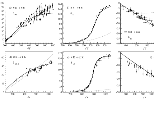
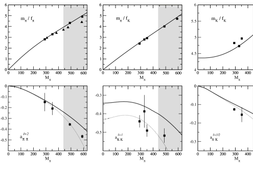
Figure 1: Results of our updated IAM fit Jeni (continuous line). We also show non-unitarized ChPT results with the LECs given in the second reference of GomezNicola:2001as (dot-dashed line). . Two upper rows: IAM versus experimental data on $\pi\pi$ and $\pi K$ scattering. Two lower rows: fit results compared to lattice calculations lattice of $f_{\pi}$, $f_{K}$, $m_{\pi}/f_{\pi}$ and the $\pi^{+}\pi^{+}$, $K^{+}K^{+}$, $K^{+}\pi^{+}$ scattering lengths. We fit up to $m_{\pi}=440MeV$, but even beyond lattice results are well described (grey areas). Experimental references are detailed in GomezNicola:2001as .

2.2 Other unitarization techniques within the coupled channel formalism

Naively one can arrive to (6) in a matrix form, ensuring coupled channel unitarity, just by expanding the real part of the inverse $T$ matrix. Unfortunately, there is still no dispersive derivation including a left cut for the coupled channel case. Being much more complicated, different approximations to ${\mbox{Re}\,}T^{-1}$ have been used:

$\bullet$ The fully renormalized one-loop ChPT calculation of ${\mbox{Re}\,}T^{-1}$ provides the correct ChPT expansion in all channels, also with left cuts approximated to $O(p^{4})$ Guerrero:1998ei ; GomezNicola:2001as . Indeed, using LECs consistent with previous determinations within standard ChPT, it was possible GomezNicola:2001as to describe below 1.2 GeV all the scattering channels of two body states made of pions, kaons or etas. Simultaneously, this approach GomezNicola:2001as generates poles associated to the $\rho(770)$ and $K^{*}(892)$ vector mesons, together with the $f_{0}(980)$, $a_{0}(980)$, $f_{0}(600)$ and $\kappa$ (or $K_{0}(800)$) scalar resonances.

$\bullet$ Originally Oller:1997ng , the coupled channel IAM was used neglecting the crossed loops and tadpoles. This approach is considerably simpler, and although it is true that the left cut is absent, its numerical influence was shown to be rather small, since the meson-meson data are nicely described with very reasonable chiral parameters and generates all the poles enumerated above. Let us remark that this approximation keeps the s-channel loops but also the tree level up to $O(p^{4})$, and that this tree level encodes the effect of heavier resonances, like the rho. Thus, contrary to some common belief, this approach still incorporates, for instance, the low energy effects of t-channel rho exchange.

$\bullet$ Finally, if only scalar meson-meson scattering is of interest, it is possible to use just one cutoff (or a dimensional regularization scale or a subtraction constant) that numerically mimics the combination of chiral parameters that appear in those scalar channels. This method – known as the ”‘chiral unitary approach”’– has become very popular, even beyond the meson-meson interaction realm, due to its great simplicity but remarkable success Oller:1997ti and also because it is rather simple to relate to the Bethe-Salpeter formalism Nieves:1998hp that provides additional physical insight on unitarization.

With this method it has been shown Oller:2003vf that, in the SU(3) limit, and assuming no quark mass dependence on the cutoff, all light scalar resonances degenerate into an octet and a singlet.

Also with this method, but using a chiral Lagrangian for the pseudoscalar-vector interaction it has been possible to generate axial-vector mesons Lutz:2003fm .

3 The nature of resonances from their leading $1/N_{c}$ behavior

The QCD $1/N_{c}$ expansion 'tHooft:1973jz , valid in the whole energy region, provides a rigorous definition of $\bar{q}q$ bound states: their masses and widths behave as $O(1)$ and $O(1/N_{c})$, respectively. The QCD leading $1/N_{c}$ behavior of $f_{\pi}$ and the LECs is well known, and ChPT amplitudes have no cutoffs or subtraction constants where spurious $N_{c}$ dependences could hide. Hence, by scaling with $N_{c}$ the ChPT parameters in the IAM, the mass and width $N_{c}$ dependence of the resonances has been determined to one and two loops Pelaez:2003dy ; Pelaez:2006nj . These are defined from the pole position as $\sqrt{s_{pole}}=M-i\Gamma$. However, a priori, one should be careful not to take $N_{c}$ too large, and in particular to avoid the $N_{c}\to\infty$ limit, because it is a weakly interacting limit. As shown above, the IAM relies on the fact that the exact elastic $RC$ contribution dominates the dispersion relation. Since the IAM describes data and the resonances within, say, 10 to 20% errors, this means that at $N_{c}=3$ the other contributions are not approximated badly. But meson loops, responsible for the $RC$, scale as $3/N_{c}$ whereas the inaccuracies due to the approximations scale partly as $O(1)$. Thus, we can estimate that those 10 to 20% errors at $N_{c}=3$ may become 100% errors at, say $N_{c}\sim 30$ or $N_{c}\sim 15$, respectively. Hence we have never shown results Pelaez:2003dy ; Pelaez:2006nj beyond $N_{c}=30$, and even beyond $N_{c}\sim 15$ they should be interpreted with care. Of course, in special cases the IAM could still work for very large $N_{c}$, as it is has been shown for the vector channel Nieves:2009ez . But that is not the case for the scalar channel, which, if used for too large $N_{c}$, leads to inconsistencies Nieves:2009ez for some values of the LECs.

Thus, Fig.2 shows the behavior of the $\rho$, $K^{*}$ and $\sigma$ masses and widths found in Pelaez:2003dy . The $\rho$ and $K^{*}$ neatly follow the expected behavior for a $\bar{q}q$ state: $M\sim 1$, $\Gamma\sim 1/N_{c}$. The bands cover the uncertainty in $\mu\sim 0.5-1$ GeV where the LECs are scaled with $N_{c}$. Note also in Fig.2 (top-right) that, for that set of LECs, outside this $\mu$ range the $\rho$ meson starts deviating from a a $\bar{q}q$ behavior. Something similar occurs to the $K^{*}(892)$. Consequently, we cannot apply the $N_{c}$ scaling at an arbitrary $\mu$ value, if the well established $\rho$ and $K^{*}$ $\bar{q}q$ nature is to be reproduced.

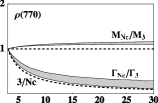
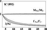
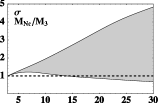
Figure 2: Top: (Left and center) $N_{c}$ behavior of the $\rho$ and $K^{*}$ mass and width. (Right) Different $\rho$ pole trajectories for different values of $\mu$, note that for $\mu=1.2$ GeV the $\rho$ pole goes away the real axis. Bottom: (Left and center) $N_{c}$ behavior of the $\sigma$ mass and width. (Right) Different $\sigma$ pole trajectories for different $\mu$ values.

In contrast, the $\sigma$ shows a different behavior from that of a pure $\bar{q}q$: near $N_{c}$=3 both its mass and width grow with $N_{c}$, i.e. its pole moves away from the real axis. Of course, far from $N_{c}=3$, and for some choices of LECs and $\mu$, the sigma pole might turn back to the real axis Pelaez:2006nj ; Nieves:2009ez ; Sun:2004de , as seen in Fig.2 (bottom-right). But, as commented above, the IAM is less reliable for large $N_{c}$, and at most this behavior only suggests that there might be a subdominant $\bar{q}q$ component Pelaez:2006nj . In addition, we have to ensure that the LECs used fit data and reproduce the vector $\bar{q}q$ behavior.

Since loops are important in determining the scalar pole position, but are $1/N_{c}$ suppressed compared to tree level terms with LECs, it is relevant to check the $O(p^{4})$ results with an $O(p^{6})$ IAM calculation. This was done within $SU(2)$ ChPT in Pelaez:2006nj . We defined a $\chi^{2}$-like function to measure how close a resonance is from a $\bar{q}q$ $N_{c}$ behavior. First, we used that $\chi^{2}$-like function at $O(p^{4})$ to show that it is not possible for the $\sigma$ to behave predominantly as a $\bar{q}q$ while describing simultaneously the data and the $\rho$ $\bar{q}q$ behavior, thus confirming the robustness of the conclusions for $N_{c}$ close to 3. Next, we obtained a $O(p^{6})$ data fit – where the $\rho$ $\bar{q}q$ behavior was imposed – whose $N_{c}$ behavior for the $\rho$ and $\sigma$ mass and width is shown in Fig.3 (left and center). Note that both $M_{\sigma}$ and $\Gamma_{\sigma}$ grow with $N_{c}$ near $N_{c}=3$, confirming the $O(p^{4})$ result of a non $\bar{q}q$ dominant component. However, as $N_{c}$ grows further, between $N_{c}\sim 8$ and $N_{c}\sim 15$, where we still trust the IAM results, $M_{\sigma}$ becomes constant and $\Gamma_{\sigma}$ starts decreasing. This may hint to a subdominant $\bar{q}q$ component, arising as loop diagrams become suppressed when $N_{c}$ grows. Finally, and despite this scenario is disfavored since the $\rho$ starts deviating from its $\bar{q}q$ behavior, we checked how big this $\sigma$ $\bar{q}q$ component can be made. Thus we forced the $\sigma$ to behave as a $\bar{q}q$ using the above mentioned $\chi^{2}$-like measure. We found that in the best case – Fig.3. (right) – this subdominant $\bar{q}q$ component could become dominant around $N_{c}>6-8$, at best, but always with an $N_{c}\to\infty$ mass above roughly 1 GeV instead of its physical $\sim 450$ MeV value.

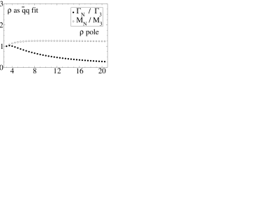
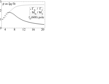
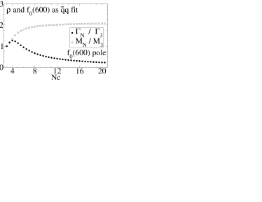
Figure 3: Left and center: $N_{c}$ behavior of the $\rho$ and $\sigma$ pole at $O(p^{6})$ with the “$\rho$ as $\bar{q}q$ fit”. Right: Sigma behavior with $N_{c}$ at $O(p^{6})$ with the “$\rho$ and $\sigma$ as $\bar{q}q$ fit”.

Let us emphasize again Pelaez:2005fd what can and what cannot be concluded from our results and clarify some frequent questions and doubts raised in this and other meetings, private discussions and the literature:

• The dominant component of the $\sigma$ and $\kappa$ in meson-meson scattering does not behave as a $\bar{q}q$. Why “dominant”? Because, most likely, scalars are a mixture of different states. If the $\bar{q}q$ was dominant, they would behave as the $\rho$ or the $K^{*}$ in Fig.2. But a smaller fraction of $\bar{q}q$ cannot be excluded and is somewhat favored in our $O(p^{6})$ analysis Pelaez:2006nj .

• Two meson and some tetraquark states Jaffe have a consistent “qualitative” behavior, i.e., both disappear in the meson-meson scattering continuum as $N_{c}$ increases. Our results are not able yet to establish the nature of that dominant component. To do so other tools might be necessary as, for instance, those outlined in Weinberg ; baru . The most we could state is that the behavior of two-meson states or some tetraquarks might be qualitatively consistent.

The $N_{c}\rightarrow\infty$ limit has been studied in Sun:2004de ; Nieves:2009ez . Apart from its mathematical interest, it could have some physical relevance if the data and the large $N_{c}$ uncertainty on the choice of scale were more accurate. Nevertheless:

• As commented above, a priori the IAM is not reliable in the $N_{c}\rightarrow\infty$ limit, since it corresponds to a weakly interacting theory, where exact unitarity becomes less relevant in confront of other approximations made in the IAM derivation. It has been shown Nieves:2009ez that it might work well in that limit in the vector channel of QCD but not in the scalar channel.

• Another reason to limit ourselves to $N_{c}$ not too far from 3 is that in our calculations we have not included the $\eta^{\prime}(980)$, whose mass is related to the $U_{A}(1)$ anomaly and scales as $\sqrt{3/N_{c}}$. Nevertheless, if in our calculations we keep $N_{c}<30$, its mass would be $>310\,$MeV and thus pions are still the only relevant degrees of freedom for the scalar channel in the $\sigma$ region.

• Contrary to the leading $1/N_{c}$ behavior in the vicinity of $N_{c}=3$, the $N_{c}\rightarrow\infty$ limit does not give information on the “dominant component” of light scalars. The reason was commented above: In contrast to $\bar{q}q$ states, that become bound, two-meson and some tetraquark states dissolve in the continuum as $N_{c}\rightarrow\infty$. Thus, even if we started with an infinitesimal $\bar{q}q$ component in a resonance, for a sufficiently large $N_{c}$ it may become dominant, and beyond that $N_{c}$ the associated pole would behave as a $\bar{q}q$ state. Also, since the mixings of different components could change with $N_{c}$, a too large $N_{c}$ could alter significantly the original mixings.

Actually, this is what happens for the one-loop IAM $\sigma$ resonance for $N_{c}\to\infty$, but it does not necessarily mean that the “correct interpretation […] is that the $\sigma$ pole is a conventional $\bar{q}q$ meson environed by heavy pion clouds” Sun:2004de . That the scalars are not conventional, is simply seen by comparing them in Figs.1 and 2 with the “conventional” $\rho$ and $K^{*}$ in those very same figures. A large two-meson component is consistent, but the $N_{c}\rightarrow\infty$ of the one-loop unitarized ChPT pole in the scalar channel limit is not unique Sun:2004de ; Nieves:2009ez given the uncertainty in the chiral parameters. Moreover, for some LECs the scalar channel one-loop IAM in the $N_{c}\rightarrow\infty$ limit can lead to phenomenological inconsistencies Nieves:2009ez , since poles can even move to negative squared mass values (weird), to infinity or to a positive mass square. That is one of the reasons why in the figures here and in Pelaez:2003dy ; Pelaez:2006nj we only plot up to $N_{c}=30$, but not 100, or a million. Hence, robust conclusions on the dominant light scalar component can be obtained not too far from real life, say $N_{c}<15$ or 30, for a $\mu$ choice between roughly $0.5$ and 1 GeV, that simultaneously ensures the $\bar{q}q$ dependence for the $\rho$ and $K^{*}$ mesons. Note, however, that under these same conditions the two-loop IAM still finds, not only a dominant non-$\bar{q}q$ component, but also a hint of a $\bar{q}q$ subdominant component, which is not conventional in the sense that it appears at a much higher mass than the physical $\sigma$. This may support the existence of a second $\bar{q}q$ scalar octet above 1 GeV VanBeveren:1986ea .

Finally, using not the IAM, but the chiral unitary approach with a natural range for the cutoff $N_{c}$ dependence, it has also been suggested Geng:2008ag that a large, in some cases dominant, non $\bar{q}q$ behavior could exist in axial vector mesons.

4 Quark mass dependence of resonances

ChPT provides a rigorous expansion of meson masses in terms of quark masses (at leading order $M_{meson}^{2}\sim m_{q}$). Thus, by changing the meson masses in the amplitudes, we see how the poles generated with the IAM depend on quark masses. In Hanhart:2008mx we presented the SU(2) analysis for the $\rho$ and $\sigma$ but here we also report on our recent developments Jeni in the SU(3) formalism and the $\kappa(800)$ and $K^{*}(892)$ strange resonances.

The values of $m_{\pi}$ considered should fall within the ChPT range of applicability and allow for some elastic $\pi\pi$ and $\pi K$ regime below $K\bar{K}$ or $K\eta$ thresholds, respectively. Both criteria are satisfied if $m_{\pi}\leq 440$ MeV, since $SU(3)$ ChPT still works with such kaon masses, and because for $m_{\pi}\simeq 440$ MeV, the kaon mass becomes $\simeq 600$ MeV. Of course, we expect higher order corrections, which are not considered here, to become more relevant as $m_{\pi}$ is increased. Thus, our results become less reliable as $m_{\pi}$ increases due to the $O(p^{6})$ corrections which we have neglected

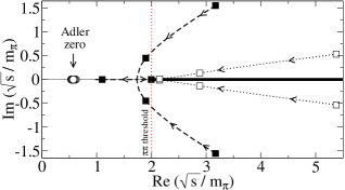
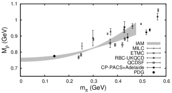
Figure 4: Left: Movement of the $\sigma$ (dashed lines) and $\rho$ (dotted lines) poles for increasing $m_{\pi}$ (direction indicated by the arrows) on the second sheet. The filled (open) boxes denote the pole positions for the $\sigma$ ($\rho$) at pion masses $m_{\pi}=1,\ 2,$ and $3\times m_{\pi}^{\rm phys}$, respectively. For $m_{\pi}=3m_{\pi}^{\rm phys}$ three poles accumulate in the plot very near the $\pi\pi$ threshold. Note that all poles are always far enough from the Adler zero (circles). Right: Comparison of our results for the $M_{\rho}$ dependence on $m_{\pi}$ with some recent lattice results from lattice1 . The grey band covers only the error coming from the LECs uncertainties.

Fig. 4 (left) shows the evolution of the $\sigma$ and $\rho$ pole positions as $m_{\pi}$ is increased. In order to see the pole movements relative to the two pion threshold, which is also increasing, all quantities are given in units of $m_{\pi}$, so the threshold is fixed at $\sqrt{s}=2$. Both poles move closer to threshold and they approach the real axis. The $\rho$ poles reach the real axis as the same time that they cross threshold. One of them jumps into the first sheet and stays below threshold in the real axis as a bound state, while its conjugate partner remains on the second sheet practically at the very same position as the one in the first. In contrast, the $\sigma$ poles go below threshold with a finite imaginary part before they meet in the real axis, still on the second sheet, becoming virtual states. As $m_{\pi}$ is increased further, one of the poles moves toward threshold and jumps through the branch point to the first sheet staying in the real axis below threshold, very close to it as $m_{\pi}$ keeps growing. The other $\sigma$ pole moves down in energies further from threshold and remains on the second sheet. These very asymmetric poles could be a signal of a prominent molecular component Weinberg ; baru , at least for large pion masses. Similar movements have been found within quark models vanBeveren:2002gy and a finite density analysis FernandezFraile:2007fv .

Fig. 4 (right) shows our results for the $\rho$ mass dependence on $m_{\pi}$ compared with some recent lattice results lattice1 , and the PDG value for the $\rho$ mass. Now the mass is defined as the point where the phase shift crosses $\pi/2$, except for those $m_{\pi}$ values where the $\rho$ becomes a bound state, where it is defined again from the pole position. Taking into account the incompatibilities within errors between different lattice collaborations, we find a qualitative good agreement with the lattice results. Also, we have to consider that the $m_{\pi}$ dependence in our approach is correct only up to NLO in ChPT, and we expect higher order corrections to be important for large pion masses. The $M_{\rho}$ dependence on $m_{\pi}$ agrees nicely with the estimations for the two first coefficients of its chiral expansion bruns .

In Fig. 5 (left) we compare the $m_{\pi}$ dependence of $M_{\rho}$ and $M_{\sigma}$ (defined from the pole position $\sqrt{s_{pole}}=M-i\Gamma/2$), normalized to their physical values. The bands cover the LECs uncertainties. We see that both masses grow with $m_{\pi}$, but $M_{\sigma}$ grows faster than $M_{\rho}$. Below $m_{\pi}\simeq 330$ MeV we only show one line because the two conjugate $\sigma$ poles have the same mass. Above 330 MeV, these two poles lie on the real axis with two different masses. The heavier pole goes towards threshold and around $m_{\pi}\simeq 465$ MeV moves into the first sheet, but that is beyond our applicability limit.

In the next panel of Fig. 5 we compare the $m_{\pi}$ dependence of $\Gamma_{\rho}$ and $\Gamma_{\sigma}$ normalized to their physical values: note that both widths become smaller. We compare this decrease with the expected phase space reduction as resonances approach the $\pi\pi$ threshold. We find that $\Gamma_{\rho}$ follows very well this expected behavior, which implies that the $\rho\pi\pi$ coupling is almost $m_{\pi}$ independent. In contrast, $\Gamma_{\sigma}$ deviates from the phase space reduction expectation. This suggests a strong $m_{\pi}$ dependence of the $\sigma$ coupling to two pions, necessarily present for molecular states baru ; mol .

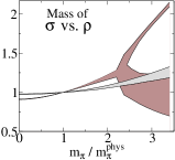
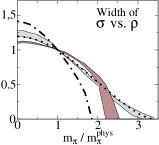
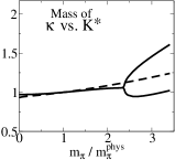
Figure 5: $m_{\pi}$ dependence of resonance masses and widths in units of the physical values. In the two left panels the dark (light) band shows the results for the $\sigma$ ($\rho$). The width of the bands reflects the uncertainties induced only from the uncertainties in the SU(2) LECs. Similarly, in the two right panels we show our recent developments Jeni for the $\kappa(800)$ and $K^{*}(892)$ using central values of the SU(3) IAM fits. The dot-dashed (dotted) line shows the $m_{\pi}$ dependence of the corresponding scalar (vector) width from the change of phase space only, assuming a constant coupling of the resonance to two mesons.

Finally, in the last two panels of Fig.5 we compare the mass and width dependence on $\hat{m}$ of the $\kappa(800)$ versus the $K^{*}(892)$, keeping $m_{s}$ fixed. Note that the same pattern of the $\sigma-\rho$ system is repeated. Belonging to the same octet, the $K^{*}(892)$ and $\rho$ behave very similarly, and both their widths follow just phase space reduction. The $\sigma$ $\kappa$ behavior are only qualitatively similar, the latter being somewhat softer. Among other effects, this might be due to a possible significant admixture of singlet state in the $\sigma$.

5 Summary

We have reviewed how the Inverse Amplitude Method (IAM) GomezNicola:2007qj is derived from the first principles of analyticity, unitarity, and Chiral Perturbation Theory (ChPT) at low energies. It is able to generate, as poles in the amplitudes, the light resonances appearing in meson-meson elastic scattering, without any a priori assumptions. Up to a given order in ChPT, it yields the correct dependences on the quark masses and the number of colors.

The resonance leading $1/N_{c}$ behavior suggests that the dominant component of light scalars does not behave as a $\bar{q}q$ state as $N_{c}$ increases not far from $N_{c}=3$. When using the two loop IAM result in SU(2), below $N_{c}\sim\,$15 or 30, there is a hint of a subdominant $\bar{q}q$ component, but arising at roughly twice the mass of the physical $\sigma$.

We have also predicted the evolution of the $f_{0}(600),\rho(770),\kappa(800)$ and $K^{*}(892)$ pole positions with increasing pion (quark) mass Hanhart:2008mx ; Jeni and have seen how they become bound states: softly in the vector case and with a non-analyticity in the scalar case. We have also shown that the vector-meson-meson coupling constant is almost $m_{\pi}$ independent and we have found a qualitative agreement with some lattice results for the $\rho$ mass evolution with $m_{\pi}$. These findings might be relevant for studies of the meson spectrum and form factors—see Ref. Guo:2008nc —on the lattice. Work is in progress Jeni to study also the strange quark mass dependence.

References

- (1) S. Weinberg, Physica A96 (1979) 327. J. Gasser and H. Leutwyler, Annals Phys. 158 (1984) 142; Nucl. Phys. B 250 (1985) 465.
- (2) G. ’t Hooft, Nucl. Phys. B 72 (1974) 461. E. Witten, Ann. Phys. 128 (1980) 363.
- (3) I. Caprini et al., Phys. Rev. Lett. 96 (2006) 132001. S. Descotes-Genon and B. Moussallam, Eur. Phys. J. C 48, 553 (2006)
- (4) T. N. Truong, Phys. Rev. Lett. 61, 2526 (1988). T. N. Truong, Phys. Rev. Lett. 67, 2260 (1991). A. Dobado, M. J. Herrero and T. N. Truong, Phys. Lett. B 235, 134 (1990).
- (5) A. Dobado and J. R. Peláez, Phys. Rev. D 47 (1993) 4883; Phys. Rev. D 56 (1997) 3057.
- (6) A. Gomez Nicola, J. R. Pelaez and G. Rios, Phys. Rev. D 77, 056006 (2008)
- (7) J. Gasser and U.-G. Meißner, Nucl. Phys. B 357 (1991) 90.
- (8) J. Nebreda and J. R. Pelaez., arXiv:1001.5237 [hep-ph]. See also J. Nebreda’s talk in this conference, arXiv:1002.1271 [hep-ph].
- (9) A. Gomez Nicola and J. R. Pelaez, Phys. Rev. D 65, 054009 (2002). AIP Conf. Proc. 660 (2003) 102. [hep-ph/0301049]. J. R. Pelaez, Mod. Phys. Lett. A 19, 2879 (2004)
- (10) S. R. Beane et al. [NPLQCD Collaboration], Phys. Rev. D 77, 094507 (2008) and Phys. Rev. D 77, 014505 (2008); S. R. Beane et al. Phys. Rev. D 74, 114503 (2006); Ph. Boucaud et al. [ETM collaboration], Comput. Phys. Commun. 179, 695 (2008).
- (11) F. Guerrero and J. A. Oller, Nucl. Phys. B 537, 459 (1999) [Erratum-ibid. B 602, 641 (2001)]
- (12) J. A. Oller, E. Oset and J. R. Pelaez, Phys. Rev. Lett. 80 (1998) 3452; Phys. Rev. D 59 (1999) 074001
- (13) J. A. Oller and E. Oset, Nucl. Phys. A 620, 438 (1997) [Erratum-ibid. A 652, 407 (1999)] and Phys. Rev. D 62 (2000) 114017.
- (14) J. Nieves and E. Ruiz Arriola, Phys. Lett. B 455, 30 (1999)
- (15) J. A. Oller, Nucl. Phys. A 727, 353 (2003)
- (16) M. F. M. Lutz and E. E. Kolomeitsev, Nucl. Phys. A 730, 392 (2004). L. Roca, E. Oset and J. Singh, Phys. Rev. D 72, 014002 (2005). L. S. Geng, E. Oset, L. Roca and J. A. Oller, Phys. Rev. D 75, 014017 (2007).
- (17) J. R. Pelaez, Phys. Rev. Lett. 92, 102001 (2004).
- (18) J. R. Pelaez and G. Rios, Phys. Rev. Lett. 97, 242002 (2006)
- (19) J. Nieves and E. R. Arriola, Phys. Rev. D 80, 045023 (2009)
- (20) Z. X. Sun, et al.[arXiv:hep-ph/0411375] and Z. X. Sun, et al.[arXiv:hep-ph/0503195].
- (21) J. R. Pelaez, arXiv:hep-ph/0509284. Proceedings of the 11th International Conference on Elastic and Diffractive Scattering, Blois, France, 15-20 May 2005. J. R. Pelaez and G. Rios, arXiv:0905.4689 [hep-ph]. Proceedings of Excited QCD, Zakopane, Poland, 8-14 Feb 2009.
- (22) R. L. Jaffe, Proc. of the Intl. Symposium on Lepton and Photon Interactions at High Energies. Physikalisches Institut, Univ. of Bonn (1981). ISBN: 3-9800625-0-3.
- (23) E. Van Beveren, et al. Z. Phys. C 30, 615 (1986) and hep-ph/0606022. E. van Beveren and G. Rupp, Eur. Phys. J. C 22 (2001) 493, J. A. Oller and E. Oset, Phys. Rev. D 60 (1999) 074023. F. E. Close and N. A. Tornqvist, J. Phys. G 28, R249 (2002).
- (24) L. S. Geng, E. Oset, J. R. Pelaez and L. Roca, Eur. Phys. J. A 39, 81 (2009)
- (25) C. Hanhart, J. R. Pelaez and G. Rios, Phys. Rev. Lett. 100, 152001 (2008)
- (26) D. Morgan, Nucl. Phys. A 543 (1992) 632; D. Morgan and M. R. Pennington, Phys. Rev. D 48 (1993) 1185.
- (27) V. Baru et al., Phys. Lett. B 586 (2004) 53.
- (28) E. van Beveren et al., AIP Conf. Proc. 660, 353 (2003); Phys. Rev. D 74, 037501 (2006).
- (29) D. Fernandez-Fraile, A. Gomez Nicola and E. T. Herruzo, Phys. Rev. D 76, 085020 (2007)
- (30) Ph. Boucaud et al. [ETM Collaboration], Phys. Lett. B 650, 304 (2007) C. Allton et al. [RBC and UKQCD Collaborations], Phys. Rev. D 76, 014504 (2007) C. W. Bernard et al.,Phys. Rev. D 64, 054506 (2001) C. R. Allton et al.Phys. Lett. B 628, 125 (2005) M. Gockeler et al.[QCDSF Collaboration], [arXiv:hep-lat/0810.5337].
- (31) P. C. Bruns and U.-G. Meißner, Eur. Phys. J. C 40 (2005) 97.
- (32) S. Weinberg, Phys. Rev. 130, 776 (1963); Y. Kalashnikova et al., Eur. Phys. J. A 24 (2005) 437.
- (33) F. K. Guo, C. Hanhart, F. J. Llanes-Estrada and U. G. Meissner, Phys. Lett. B 678, 90 (2009)