Reentrant fractional quantum Hall states in bilayer graphene: Controllable, driven phase transitions

Abstract

Here we report from our theoretical studies that in biased bilayer graphene, one can induce phase transitions from an incompressible state to a compressible state by tuning the bandgap at a given electron density. Likewise, variation of the density with a fixed bandgap results in a transition from the FQHE states at lower Landau levels to compressible states at intermediate Landau levels and finally to FQHE states at higher Landau levels. This intriguing scenario of tunable phase transitions in the fractional quantum Hall states is unique to bilayer graphene and never before existed in conventional semiconductor systems.

The unconventional quantum Hall effect in monolayer graphene, whose experimental observation novoselov_kim unleashed quite unprecedented interest in this system review , reflects the unique behavior of massless Dirac fermions in a magnetic field wallace ; mcclure . In bilayer graphene this effect confirms the presence of massive chiral quasiparticles novoselov_bi . An important characteristic of bilayer graphene is that it is a semiconductor with a tunable bandgap between the valence and conduction bands pereira . This modifies the Landau level spectrum and influences the role of long-range Coulomb interactions abergel . Here we report that the fractional quantum Hall effect (FQHE), a distinct signature of interacting electrons in the system fqhe_book ; stormer is very sensitive to the interlayer coupling strength and the bias voltage. We propose that by tuning the bias voltage, one can induce phase transitions from an incompressible state to a compressible state at a given gate voltage. In the same vein, variation of the gate voltage at a fixed bias potential results in a transition from the FQHE states in lower Landau levels to compressible states in intermediate Landau levels and finally to FQHE states in higher Landau levels. This interesting scenario of tunable phase transitions in the FQH states is unique to bilayer graphene and never before existed in conventional semiconductor systems. The FQHE in monolayer graphene was in fact, studied theoretically by us vadim_fqhe and subsequent experiments confirmed the existence of that effect in suspended monolayer graphene samples fqhe_kim . No such studies have been reported on bilayer graphene.

We assume that the bilayer graphene consists of two coupled graphene layers with the Bernal stacking arrangement. In that case, we are mainly concerned with the coupling between the atoms of sublattice A of the lower layer and atoms of sublattice B^′ of the upper layer. The single-particle levels in bilayer graphene have two-fold spin degeneracy and two-fold valley degeneracy, which can be lifted in many-particle systems at relatively large magnetic fields nakamura . Considering only one valley (say valley K) and one direction of spin, we describe the state of the bilayer system in terms of the four-component spinor $(\psi_{A},\psi_{B},\psi_{B^{\prime}},\psi_{A^{\prime}})^{T}$. Here subindices A, B and A^′, B^′ correspond to lower and upper layers respectively. The strength of inter-layer coupling is described in terms of the inter-layer hopping integral, $t$. In a biased bilayer graphene the bias potential is introduced as the potential difference, $\Delta U$, between the upper and lower layers. The Hamiltonian of the biased bilayer system in a perpendicular magnetic field then takes the following form

$${\cal H}=\left(\begin{array}[]{cccc}\Delta U/2&v_{F}\pi_{+}&t&0\\ v_{F}\pi_{-}&\Delta U/2&0&0\\ t&0&-\Delta U/2&v_{F}\pi_{-}\\ 0&0&v_{F}\pi_{+}&-\Delta U/2\end{array}\right),$$ (1)

where $\pi_{\pm}=\pi_{x}\pm i\pi_{y}$, $\vec{\pi}=\vec{p}+e\vec{A}/c$, $\vec{p}$ is an electron two-dimensional momentum, $\vec{A}$ is the vector potential, and $v_{F}\approx 10^{6}$ m/s is the fermi velocity.

In a perpendicular magnetic field the Hamiltonian (1) generates a discrete Landau level energy spectrum. The corresponding eigenfunctions can be expressed in terms of the conventional nonrelativistic Landau functions. The electron states at sublattices A and A^′ are expressed in terms of the $n$-th ‘nonrelativistic’ Landau functions, while the electron states at sublattices B and B^′ are described by the $|n-1|$ and $n+1$ Landau functions, respectively. Therefore the Landau states in bilayer graphene can be described as a mixture of the $n$, $n+1$, and $n-1$ nonrelativistic Landau functions belonging to different sublattices pereira . This mixture, for a given value of $n$, results in four different Landau levels in bilayer graphene. The energies, $\varepsilon$, of the four Landau levels corresponding to the index $n$ can be found from the following equation pereira

$$\left[\left(\varepsilon+\delta\right)^{2}-2(n+1)\right]\left[(\varepsilon-\delta)^{2}-2n\right]=(\varepsilon^{2}-\delta^{2})t^{2},$$ (2)

where $\delta=\Delta U/2$ and all energies are expressed in units of $\hbar v_{F}/l_{B}$. Here $l_{B}=(\hbar/eB)^{\frac{1}{2}}$ is the magnetic length.

It is convenient to introduce special labeling of the Landau levels in bilayer graphene. From Eq. (2), we can see that for each value of $n$, $n=0,1,2,\ldots$, there are four solutions, i.e., four Landau levels. Then each of these Landau levels can be labeled as $n_{(i)}$, where $i=1,...,4$ is the number of the Landau level corresponding to the solution of Eq. (2) for a given value of $n$.

For a partially occupied Landau level, the properties of the system, e.g., the ground state and excitations, are completely determined by the inter-electron interactions, which can be expressed by Haldane’s pseudopotentials, $V_{m}$, haldane which are the energies of two electrons with relative angular momentum $m$. In a graphene bilayer the Haldane pseudopotentials in a Landau level with index $n$ and the energy $\varepsilon$ have the form

$$V_{m}^{(n)}=\int_{0}^{\infty}\frac{dq}{2\pi}qV(q)\left[F_{n,\varepsilon}(q)\right]^{2}L_{m}(q^{2})e^{-q^{2}},$$ (3)

where $L_{m}(x)$ are the Laguerre polynomials, $V(q)=2\pi e^{2}/(\kappa l_{B}q)$ is the Coulomb interaction in the momentum space, $\kappa$ is the dielectric constant, and $F_{n,\varepsilon}(q)$ are the corresponding form factors

$$F_{n,\varepsilon}(q)= d_{n}^{2}\left[\left(1+f_{n}^{2}\right)L_{n}\left(\tfrac{q^{2}}{2}\right)+\frac{2n}{(\varepsilon-\delta)^{2}}L_{n-1}\left(\tfrac{q^{2}}{2}\right)\right.$$ (4)

$$+\left.\frac{2(n+1)}{(\varepsilon+\delta)^{2}}f_{n}^{2}L_{n+1}\left(\tfrac{q^{2}}{2}\right)\right],$$

where $f_{n}=[(\varepsilon-\delta)^{2}-2n]/[t(\varepsilon-\delta)]$ and

$$d_{n}=\left[1+f_{n}^{2}+\frac{2n}{(\varepsilon-\delta)^{2}}+\frac{2(n+1)}{(\varepsilon+\delta)^{2}}f_{n}^{2}\right]^{-\frac{1}{2}}.$$ (5)

The form factors of bilayer graphene [Eq. (4)] are clearly different from the corresponding form factors of a single layer of graphene. For a single layer of graphene, the form factor of the $n=0$ Landau level is the same as that of conventional non-relativistic electrons vadim_fqhe ; goerbig , $F_{n=0}(q)=L_{0}\left(q^{2}/2\right)$. The form factors of higher Landau levels are determined by the mixture of $L_{n}$ and $L_{n+1}$ terms. For bilayer graphene the form factors of the Landau level with index $n=0$ are the mixtures of the $L_{0}$ and $L_{1}$ terms and are different from that in the non-relativistic case. There is of course, one special Landau level in bilayer graphene with index $n=0$, whose properties are completely identical to that of the non-relativistic $n=0$ Landau level. Indeed, it is clear from Eq. (2) that at $n=0$ there is a Landau level with energy $\epsilon=\delta$. This energy does not depend on the coupling between the layers, i.e., the inter-layer hopping integral, $t$. The form factor of this Landau level is exactly equal to the form factor of a non-relativistic system of the $n=0$ Landau level, $F_{n=0,\epsilon=\delta}=L_{0}$. Therefore, all many-body properties of a bilayer system in the $n=0$, $\epsilon=\delta$ Landau level are completely identical to those of a non-relativistic conventional system in the $n=0$ Landau level.

For Landau levels with higher indices the form factor is the mixture of three different functions, $L_{n}$, $L_{n-1}$, and $L_{n+1}$. Therefore, in general, the strength of inter-electron interactions in bilayer graphene is strongly modified as compared to its value in monolayer graphene. To address the effects of these modifications on the properties of the many-electron system in a graphene bilayer we study below the partially occupied Landau levels with fractional filling factor corresponding to the FQHE fqhe_book . In what follows, we study the many-electron system at various fractional filling factors numerically within the spherical geometry vadim_fqhe ; haldane . The radius of our spehere is $R=\sqrt{S}l_{B}$, where $2S$ is the number of magnetic fluxes through the sphere in units of the flux quanta. The single-electron states are characterized by the angular momentum, $S$, and its $z$ component, $S_{z}$. For the many-electron system the corresponding states are classified by the total angular momentum $L$ and its $z$ component, while the energy of the state depends only on $L$ fano . A given fractional filling of the Landau level is determined by a special relation between the number of electrons $N$ and the radius of the sphere $R$. For example, the $\frac{1}{3}$-FQHE state is realized at $S=(\frac{3}{2})(N-1)$, while the $\frac{2}{5}$-FQHE state corresponds to the relation $S=(\frac{5}{4})N-2$. With the Haldane pseudopotentials [Eq. (3)] we determine the interaction Hamiltonian matrix fano and then calculate a few lowest eigenvalues and eigenvectors of this matrix. The FQHE states are obtained when the ground state of the system is an incompressible liquid, the energy spectrum of which has a finite many-body gap fqhe_book ; stormer .

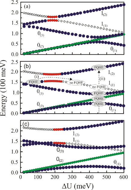
Figure 1: A few lowest Landau levels of the conduction band are shown as a function of the bias potential, $\Delta U$, for different values of inter-layer coupling: (a) $t=100$ meV (b) $t=200$ meV and (c) $t=400$ meV and the magnetic field is 15 Tesla. The numbers next to the curves denote the corresponding Landau levels. The Landau levels where the FQHE can be observed are drawn as blue and green dots. The green dots correspond to the Landau levels where the FQHE states are identical to that of a monolayer of graphene or a non-relativistic conventional system. The red dots represent Landau levels with weak FQHE. The open dots correspond to the Landau levels where the FQHE cannot be observed. In (b), the dashed lines labeled by (i) and (ii) illustrate two situations: (i) under a constant gate voltage and variable bias potential; (ii) under a constant bias potential and variable gate voltage.

We begin our study with the celebrated $\frac{1}{3}$-FQHE stormer corresponding to the filling factor $\nu=\frac{1}{3}$. In Fig. 1 we show the behavior of the Landau level spectra as a function of the bias voltage and for different values of the inter-layer hopping integral, $t$. Only the Landau levels with positive energies (corresponding to the conduction band) are shown in the figure. A similar behavior is valid for other FQHE filling factors, e.g., for $\nu=\frac{2}{5}$. Figure 1 clearly illustrates that the FQHE can be observed in all $n=0$ Landau levels with the strongest FQHE being in the first and the third $n=0$ Landau levels, i.e., $0_{(1)}$ and $0_{(3)}$. An interesting behavior was also observed for the $n=1$ Landau levels. For $\Delta U\approx 200$ meV the $n=1$ Landau levels show an anti-crossing, which is accompanied by strong changes in the properties of the FQHE. More specifically, at a small $\Delta U$ the FQHE can be observed only in the lower $n=1$ Landau level, while for larger $\Delta U$ the FQHE is possible only in higher $n=1$ Landau level. These have important implications for possible experimental observations of this unique behavior (see Fig. 1(b)):

(i) By applying a gate voltage the electron density can be tuned so that the first three Landau levels in bilayer graphene are completely occupied and the next Landau level is partially occupied with the FQHE filling factor, for example, $\nu=\frac{1}{3}$. According to the notations of Fig. 1, this means that the $0_{(1)}$, $0_{(2)}$, $0_{(3)}$ Landau levels are fully occupied, while the $1_{(1)}$ Landau level has a filling factor $\frac{1}{3}$. Then, by varying $\Delta U$ from a small value, e.g., 100 meV, to a larger value, e.g., 400 meV, one can observe the disappearance of the FQHE (see line (i) in Fig. 1(b)).

(ii) The bias voltage is kept fixed at a large value, e.g., $\Delta U=400$ meV. Then by varying the gate voltage and thus increasing the electron density, one can observe the disappearance and reappearance of the FQHE at large Landau levels (see line (ii) in Fig. 1(b)).

The appearance or suppression of the FQHE in different Landau levels is correlated with the unique behavior of Haldane pseudopotentials in bilayer graphene. The FQHE is observed in Landau levels with a rapid decrease of the corresponding pseudopotentials with increasing angular momentum, $m$. For the first and second $n=0$ Landau levels ($0_{(1)}$ and $0_{(2)}$ levels), between $m=1$ and $m=3$, the pseudopotential has the fastest decay for the first level, which results in a higher FQHE gap in this Landau level. The pseudopotentials in the $0_{(2)}$ Landau level exactly coincide with the pseudopotentials of the $n=0$ Landau level in a single layer of graphene. For the $n=1$ Landau levels, the pseudopotentials in one of the $n=1$ levels are close to those in the $n=1$ Landau level of the monolayer graphene, resulting in a well pronounced FQHE. While in the other $n=1$ Landau level of the bilayer graphene the pseudopotentials display a slow decrease with $m$ and no FQHE is expected in that Landau level.

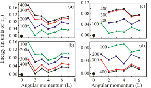
Figure 2: Low energy excitation spectra of the FQHE states shown for different values of the bias potential. The numbers next to the lines are the values of the bias potential in meV. (a) $\nu=\frac{1}{3}$-FQHE (eight electrons) system in the Landau level $1_{(2)}$, (b) $\nu=\frac{1}{3}$-FQHE (eight electrons) system in the Landau level $1_{(1)}$, (c) $\nu=\frac{2}{5}$-FQHE (ten electrons) system in the Landau level $1_{(2)}$, (d) $\nu=\frac{2}{5}$-FQHE (ten electrons) system in the Landau level $1_{(1)}$. The systems are fully spin-polarized. The flux quanta is $2S=21$. The magnetic field is 15 T. The ground state is shown as a solid dot at $L=0$.

The collapse of the FQHE gap, corresponding to the appearence of anticrossing of the $n=1$ Landau levels, is illustrated in Fig. 2. The FQHE gap has a monotonic dependence on the bias voltage. In the anticrossing region the gap disappears for the lower $n=1$ Landau level (see Fig. 2a,c) and reappears for the higher $n=1$ Landau level (see Fig. 2b,d). The evolutions of the energy spectra of the incompressible liquid with different filling factors are similar, which is illustrated in Fig. 2a,b (for $\nu=\frac{1}{3}$) and Fig. 2c,d (for $\nu=\frac{2}{5}$). This behavior was never before observed in the FQHE of conventional two-dimensional electron systems.

The strength of the FQHE effect, i.e., the magnitude of the excitation gap, depends on the parameters of the bilayer graphene, i.e., on the bias voltage and the inter-layer hopping integral, $t$. In Fig. 3 such dependence is shown for $\frac{1}{3}$- and $\frac{2}{5}$-FQHE in different Landau levels as a function of the hopping integral, $t$. In accordance with the properties of Haldane pseudopotentials, the excitation gap of the $0_{(2)}$ Landau levels does not depend on the bias voltage and on the inter-layer hopping integral. The corresponding gap remains constant and is equal to gap of the FQHE in a single layer of graphene in the $n=0$ Landau level. This gap has the smallest value compared to that of the other Landau levels. For zero hopping integral the two layers of graphene become decoupled and the bilayer system becomes identical to a single layer with additional double degeneracy. This property is clearly seen in Fig. 3, where at $t=0$ there are only two doubly degenerate FQHE gaps, corresponding to $n=0$ and $n=1$ single layer Landau levels.

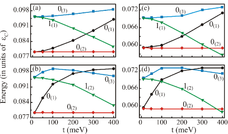
Figure 3: The FQHE gaps are shown for different Landau levels. The labels next to the lines correspond to the labeling of Landau levels shown in Fig. 1. (a) $\nu=\frac{1}{3}$-FQHE (eight electron) system at $\Delta U=10$ meV, (b) $\nu=\frac{1}{3}$-FQHE (eight electron) system at $\Delta U=400$ meV, (c) $\nu=\frac{2}{5}$-FQHE (ten electron) system at $\Delta U=10$ meV, (d) $\nu=\frac{2}{5}$-FQHE (ten electron) system at $\Delta U=400$ meV. All systems are fully spin polarized. The flux quanta is $2S=21$. The magnetic field is 15 Tesla.

At a small bias voltage ($\Delta U=10$ meV, see Fig. 3a,c), the FQHE gaps have a monotonic dependence on the hopping integral. The values of the gaps increases for the $n=0$ Landau levels, while for the $n=1$ Landau level the gap decreases. At large values of the bias voltage, $\Delta U=400$ meV (see Fig. 3b,d), the FQHE gap in the $0_{3}$ Landau level has a nonmonotonic dependence on the hopping integral with a maximum around $t=100$ meV. These results also illustrate that the FQHE in bilayer graphene can be more stable, i.e., the corresponding FQHE gap is much larger than in the case of FQHE in a single graphene layer. As an illustration, the FQHE gaps in the $0_{(1)}$ and $0_{(3)}$ Landau levels at finite values of $t$ are larger than the FQHE gaps in a single layer of graphene, i.e., at $t=0$.

Our present work suggests an unique opportunity to tune the reentrant FQHE states. The transition from the FQHE state to a gapless compressible state is continuous. The gap decreases monotonically with the bias potential and finally collapses. The collapse of the FQHE gap occurs at a non-zero angular momentum, $L\approx 2$, resulting in the formation of the ground state with a finite momentum. Experimental observation of this transition will provide unique opportunities, for the first time, to study the phase transition from an incompressible liquid to a possible charge density wave state and then to another incompressible state.

We wish to thank David Abergel for very helpful discussions. The work has been supported by the Canada Research Chairs Program and the NSERC Discovery Grant.

References

- (1) Electronic address: tapash@physics.umanitoba.ca
- (2) K.S. Novoselov, et al., Nature 438, 197 (2005); Y. Zhang, J.W. Tan, H.L. Störmer, and P. Kim, ibid. 438, 201 (2005).
- (3) D.S.L. Abergel, V. Apalkov, J. Berashevich, K. Ziegler, and T. Chakraborty, Adv. Phys. (in press) (2010).
- (4) P.R. Wallace, Phys. Rev. 71, 622 (1947).
- (5) J.W. McClure, Phys. Rev. 104, 666 (1956).
- (6) K.S. Novoselov, et al., Nat. Phys. 2, 177 (2006); E. McCann and V. Falko, Phys. Rev. Lett. 96, 086805 (2006); E. McCann, Phys. Rev. B 74, 161403 (2006); T. Ohta, A. Bostwick, T. Seyller, K. Horn, E. Rotenberg, Science 313, 951 (2006); E.V. Castro, et al., Phys. Rev. Lett. 99, 216802 (2007).
- (7) J.M. Pereira, Jr., F.M. Peeters, and P. Vasilopoulos, Phys. Rev. B 76, 115419 (2007).
- (8) D.S.L. Abergel and T. Chakraborty, Phys. Rev. Lett. 102, 056807 (2009).
- (9) T. Chakraborty, and P. Pietiläinen, The Quantum Hall Effects (Springer, New York, 1995), 2nd edition; T. Chakraborty, Adv. Phys. 49, 959 (2000).
- (10) D.C. Tsui, H.L. Störmer, and A.C. Gossard, Phys. Rev. Lett. 48, 1559 (1982); R.B. Laughlin, ibid. 50, 1395 (1983).
- (11) V.M. Apalkov, and T. Chakraborty, Phys. Rev. Lett. 97, 126801 (2006).
- (12) K.I. Bolotin, F. Ghahari, M.D. Shulman, H.L. Störmer, and P. Kim, Nature 462, 196 (2009); see also, X. Du, et al., ibid. 462, 192 (2009).
- (13) M. Nakamura, E.V. Castro, and B. Dora, Phys. Rev. Lett. 103, 266804 (2009); Y. Zhao, P. Cadden-Zimansky, Z. Jiang, and P. Kim, ibid. 104, 66801 (2010).
- (14) F.D.M. Haldane, Phys. Rev. Lett. 51, 605 (1983).
- (15) M.O. Goerbig, R. Moessner and B. Doucot,Phys. Rev. B 74 161407(R) (2006).
- (16) G. Fano, F. Ortolani, and E. Colombo, Phys. Rev. B 34, 2670 (1986).