Abstract

We construct a two-parameter family of Bäcklund transformations for the trigonometric classical Gaudin magnet. The approach follows closely the one introduced by E.Sklyanin and V.Kuznetsov (1998,1999) in a number of seminal papers, and takes advantage of the intimate relation between the trigonometric and the rational case. As in the paper by A.Hone, V.Kuznetsov and one of the authors (O.R.) (2001) the Bäcklund transformations are presented as explicit symplectic maps, starting from their Lax representation. The (expected) connection with the xxz Heisenberg chain is established and the rational (xxx) case is recovered in a suitable limit. It is shown how to obtain a “physical” transformation mapping real variables into real variables. The interpolating Hamiltonian flow is derived and some numerical iterations of the map are presented.

KEYWORDS: Bäcklund Transformations, Integrable maps, Gaudin systems, Lax representation, r-matrix.

1 Introduction

Bäcklund transformations are nowadays a widespread useful tool related to the theory of nonlinear differential equations. The first historical evidence of their mathematical significance was given by Bianchi [3] and Bäcklund [2] on their works on surfaces of constant curvature. A simple approach to understand their importance can be to regard them as a mechanism allowing to endow a given nonlinear differential equation with a nonlinear superposition principle yielding a set of solutions through a merely algebraic procedure [19],[1],[12]. Bäcklund transformations are indeed parametric families of difference equations encoding the whole set of symmetries of a given integrable dynamical system. For finite-dimensional integrable systems the technique of Bäcklund transformations leads to the construction of integrable Poisson maps that discretize a family of continuous flows [27],[25],[24],[22],[10],[9]. Actually in the last two decades numerous results have appeared in the field of exact discretization of many-body integrable systems employing the Bäcklund transformations tools [17],[24],[16],[9],[10],[15],[22]. For the rational Gaudin model such discretization has been obtained ten years ago in [8]; afterwards, these results have been used for constructing an integrable discretization of classical dynamical systems (as the Lagrange top) connected to Gaudin model through Inönu-Wigner contractions [13],[11],[14].

The aim of the present work is to construct Bäcklund transformations for the Gaudin model in the partially anisotropic ($xxz$) case, i.e. for the trigonometric Gaudin model. We point out that partial results on this issue have already been given in [18].

The paper is organized as follows.
In Section (2) we review the main features of the trigonometric Gaudin model from the point of view of its integrability structure. For the sake of completeness, in Section (3) we briefly recall the preliminary results on Bäcklund Transformations (BTs) for trigonometric Gaudin given in [18]. In Section (4) the explicit form of BTs is given; it is shown that they are indeed a trigonometric generalization of the rational ones (see [8]) which can be recovered in a suitable (“small angle” ) limit. The simplecticity of the transformations is also discussed in the same Section and the proof allows us to elucidate the (expected) link between the Darboux-dressing matrix and the elementary Lax matrix for the $xxz$ Heisenberg magnet on the lattice. We end the Section by mentioning an open question, namely the construction of an explicit generating function for these Bäcklund transformations. In Section (5) we will show how our map can lead, with an appropriate choice of Bäcklund parameters, to physical transformations, i.e. transformations from real variables to real variables. In the last Section we show how a suitable continuous limit yields the interpolating Hamiltonian flow and finally present numerical examples of iteration of the map.

2 Gaudin magnet in the trigonometric case

For a full account of the integrability structure of the classical and quantum Gaudin model we refer the reader to the fundamental contributions by Semenov-Tian-Shanski [26] and Babelon-Bernard-Talon [4]. In this section we briefly recall the main features of the trigonometric Gaudin magnet.
The Lax matrix of the model is given by the expression:

$$L(\lambda)=\left(\begin{array}[]{cc}A(\lambda)&B(\lambda)\\ C(\lambda)&-A(\lambda)\end{array}\right)$$ (1)

$$A(\lambda)=\sum_{j=1}^{N}\cot(\lambda-\lambda_{j})s^{3}_{j},\qquad B(\lambda)=\sum_{j=1}^{N}\frac{s^{-}_{j}}{\sin(\lambda-\lambda_{j})},\qquad C(\lambda)=\sum_{j=1}^{N}\frac{s^{+}_{j}}{\sin(\lambda-\lambda_{j})}.$$ (2)

In (1) and (2) $\lambda\in\mathbb{C}$ is the spectral parameter, $\lambda_{j}$ are arbitrary real parameters of the model, while $\big{(}s^{+}_{j},s^{-}_{j},s^{3}_{j}\big{)}$,  $j=1,\ldots,N$, are the dynamical variables of the system obeying to $\oplus^{N}sl(2)$ algebra, i.e.

$$\big{\{}s^{3}_{j},s^{\pm}_{k}\big{\}}=\mp i\delta_{jk}s^{\pm}_{k},\qquad\big{\{}s^{+}_{j},s^{-}_{k}\big{\}}=-2i\delta_{jk}s^{3}_{k},$$ (3)

By fixing the $N$ Casimirs $\big{(}s_{j}^{3}\big{)}^{2}+s_{j}^{+}s_{j}^{-}\doteq s_{j}^{2}$ one obtains a symplectic manifold given by the direct sum of the correspondent $N$ two-spheres.
Reformulating the Poisson structure in terms of the $r$-matrix formalism amounts to state that the Lax matrix satisfies the linear $r$-matrix Poisson algebra (see again [26], [4]) :

$$\big{\{}L(\lambda)\otimes\hbox{$1\hskip-1.2pt\vrule depth=0.0pt,height=6.88889pt,width=0.7pt\vrule depth=0.0pt,height=0.3pt,width=1.19995pt$},\hbox{$1\hskip-1.2pt\vrule depth=0.0pt,height=6.88889pt,width=0.7pt\vrule depth=0.0pt,height=0.3pt,width=1.19995pt$}\otimes L(\mu)\big{\}}=\big{[}r_{t}(\lambda-\mu),L(\lambda)\otimes\hbox{$1\hskip-1.2pt\vrule depth=0.0pt,height=6.88889pt,width=0.7pt\vrule depth=0.0pt,height=0.3pt,width=1.19995pt$}+\hbox{$1\hskip-1.2pt\vrule depth=0.0pt,height=6.88889pt,width=0.7pt\vrule depth=0.0pt,height=0.3pt,width=1.19995pt$}\otimes L(\mu)\big{]},$$ (4)

where $r_{t}(\lambda)$ stands for the trigonometric $r$ matrix [5]:

$$r_{t}(\lambda)=\frac{i}{\sin(\lambda)}\left(\begin{array}[]{cccc}\cos(\lambda)&0&0&0\\ 0&0&1&0\\ 0&1&0&0\\ 0&0&0&\cos(\lambda)\end{array}\right),$$ (9)

Equation (4) entails the following Poisson brackets for the functions (2):

$$\{A(\lambda),A(\mu)\}=\{B(\lambda),B(\mu)\}=\{C(\lambda),C(\mu)\}=0,$$

$$\{A(\lambda),B(\mu)\}=i\frac{\cos(\lambda-\mu)B(\mu)-B(\lambda)}{\sin(\lambda-\mu)},$$

$$\{A(\lambda),C(\mu)\}=i\frac{C(\lambda)-\cos(\lambda-\mu)C(\mu)}{\sin(\lambda-\mu)},$$

$$\{B(\lambda),C(\mu)\}=i\frac{2(A(\mu)-A(\lambda))}{\sin(\lambda-\mu)}.$$ (10)

The determinant of the Lax matrix is the generating function of the integrals of motion:

$$-\textrm{det}(L)=A^{2}(\lambda)+B(\lambda)C(\lambda)=\sum_{i=1}^{N}\left(\frac{s_{i}^{2}}{\sin^{2}(\lambda-\lambda_{i})}+H_{i}\cot(\lambda-\lambda_{i})\right)-H_{0}^{2}$$ (11)

where the $N$ Hamiltonians $H_{i}$ are of the form:

$$H_{i}=\sum_{k\neq i}^{N}\frac{2\cos(\lambda_{i}-\lambda_{k})s_{i}^{3}s_{k}^{3}+s_{i}^{+}s_{k}^{-}+s_{i}^{-}s_{k}^{+}}{\sin(\lambda_{i}-\lambda_{k})}$$ (12)

Note that only $N-1$ among these Hamiltonians are independent, because of $\sum_{i}H_{i}=0$. Another integral is given by $H_{0}$, the projection of the total spin on the $z$ axis:

$$H_{0}=\sum_{j=1}^{N}s_{j}^{3}\doteq J^{3}$$ (13)

The Hamiltonians $H_{i}$ are in involution for the Poisson bracket (3):

$$\{H_{i},H_{j}\}=0\quad i,j=0,\ldots,N-1$$ (14)

The corresponding Hamiltonian flows are then given by:

$$\frac{ds^{3}_{j}}{dt_{i}}=\{H_{i},s^{3}_{j}\}\qquad\frac{ds^{\pm}_{j}}{dt_{i}}=\{H_{i},s^{\pm}_{j}\}$$ (15)

In the $xxx$ model a remarkable Hamiltonian is found by taking a linear combination of the integrals corresponding to (12) in the rational case [6]. It describes a mean field spin-spin interaction:

$$\mathcal{H}_{r}=\frac{1}{2}\sum_{i\neq j}^{N}\mathbf{s}_{i}\cdot\mathbf{s}_{j}$$

Where the notation for the bold symbol $\mathbf{s}_{i}$ is $\mathbf{s}_{i}=(s_{i}^{1},s_{i}^{2},s_{i}^{3})$ with $s_{i}^{+}=s_{i}^{1}+is_{i}^{2}$ and $s_{i}^{-}=s_{i}^{1}-is_{i}^{2}$. The natural trigonometric generalization of this Hamiltonian can be found by taking the linear combination of 12:

$$\sum_{i=1}^{N}\frac{\sin(2\lambda_{i})}{2}H_{i}$$

giving

$$\mathcal{H}_{t}=\frac{1}{2}\sum_{i\neq j}^{N}\cos(\lambda_{i}+\lambda_{j})\left(s_{i}^{1}s_{j}^{1}+s_{i}^{2}s_{j}^{2}+\cos(\lambda_{i}-\lambda_{j})s_{i}^{3}s_{j}^{3}\right)$$ (16)

3 A first approach to Darboux-dressing matrix

In this Section, for the sake of completeness, we recall the results already appeared in [18]. The leading observation is that by performing the “uniformization” mapping:

$$\lambda\to z\doteq e^{i\lambda}$$

the $N$-sites trigonometric Lax matrix takes a rational form in $z$ that corresponds to the $2N$-sites rational Lax matrix plus an additional reflection symmetry (see also [7]); in fact, by performing the substitution (3), the Lax matrix (1) becomes:

$$L(z)=iJ^{3}+\sum_{j=1}^{N}\left(\frac{L_{1}^{j}}{z-z_{j}}-\sigma_{3}\frac{L_{1}^{j}}{z+z_{j}}\sigma_{3}\right),$$ (17)

where $\sigma_{3}$ is the Pauli matrix $diag(1,-1)$ and the matrices $L_{1}^{j}$,   $j=1,\ldots,N$, are given by:

$$L_{1}^{j}=iz_{j}\left(\begin{array}[]{cc}s_{j}^{3}&s_{j}^{-}\vspace{1mm}\\ s_{j}^{+}&-s_{j}^{3}\end{array}\right)$$

So, equation (17) entails the following involution on $L(z)$:

$$L(z)=\sigma_{3}L(-z)\sigma_{3}$$ (18)

Constructing a Bäcklund transformation for the Trigonometric Gaudin System (TGS) amounts to build up a Poisson map for the field variables of the model (2) such that the integrals of motion (12) are preserved. At the level of Lax matrices, this transformation is usually seeked as a similarity transformation between an old, or “undressed”, Lax matrix $L$, and a new, or “dressed” one, say $\tilde{L}$:

$$L(z)\to D(z)L(z)D^{-1}(z)\equiv\tilde{L}(z)$$ (19)

But $L$ and $\tilde{L}$ have to enjoy the same reflection symmetry (18) too: to preserve this involution the Darboux dressing matrix $D$ has to share with $L$ the property (18); the elementary dressing matrix $D$ is then obtained by requiring the existence of only one pair of opposite poles for $D$ in the complex plane of the spectral parameter. We will show in the next Section that, thanks to this constraint, one recovers the form of the Lax matrix for the elementary $xxz$ Heisenberg spin chain: on the other hand, this is quite natural if one recalls that for the rational Gaudin model the elementary Darboux-dressing matrix is given by the Lax matrix for the elementary $xxx$ Heisenberg spin chain [8],[10]. The previous observations lead to the following Darboux matrix:

$$D(z)=D_{\infty}+\frac{D_{1}}{z-\xi}-\sigma_{3}\frac{D_{1}}{z+\xi}\sigma_{3}$$ (20)

By taking the limit $z\to\infty$ in (20) it is readily seen that $D_{\infty}$ has to be a diagonal matrix. In order to ensure that $L$ and $\tilde{L}$ have the same rational structure in $z$, we rewrite equation (19) in the form:

$$\tilde{L}(z)D(z)=D(z)L(z)$$ (21)

Now it is clear that both sides have the same residues at the poles $z=z_{j}$, $z=\xi_{j}$ (it is unnecessary to look at the poles in $z=-z_{j}$ and $z=-\xi_{j}$ because of the symmetry (18), so that the following set of equations have to be satisfied:

$$\tilde{L}_{1}^{(j)}D(z_{j})=D(z_{j})L_{1}^{(j)},$$ (22)

$$\tilde{L}(\xi)D_{1}=D_{1}L(\xi).$$ (23)

In principle, equations (22), (23) yield a Darboux matrix depending both on the old (untilded) variables and the new (tilded) ones, implying in turn an implicit relationship between the same variables. To get an explicit relationship one has to resort to the so-called spectrality property [10] [9]. To this aim we need to force the determinant of the Darboux matrix $D(z)$ to have, besides the pair of poles at $z=\pm\xi$, a pair of opposite nondynamical zeroes, say at $z=\pm\eta$, and to allow the matrix $D_{1}$ to be proportional to a projector [18]. Again by symmetry it suffices to consider just one of these zeroes. If $\eta$ is a zero of det$D(z)$, then $D(\eta)$ is a rank one matrix, possessing a one dimensional kernel $|K(\eta)\rangle$; the equation (21) :

$$\tilde{L}(\eta)D(\eta)=D(\eta)L(\eta)$$ (24)

entails

$$D(\eta)L(\eta)|K(\eta)\rangle=0.$$ (25)

This equation in turn allows to infer that $|K(\eta)\rangle$ is an eigenvector for the Lax matrix $L(\eta)$:

$$L(\eta)|K(\eta)\rangle=\mu(\eta)|K(\eta)\rangle,$$ (26)

This relations gives a direct link between the parameters appearing in the dressing matrix $D$ and the old dynamical variables in $L$. Because of (23) we have another one dimensional kernel $|K(\xi)\rangle$ of $D_{1}$, such that:

$$L(\xi)|K(\xi)\rangle=\mu(\xi)|K(\xi)\rangle.$$ (27)

In [18] we have shown how the two spectrality conditions (26), (27) enable to write $D$ in terms of the old dynamical variables and of the two Bäcklund parameters $\xi$ and $\eta$. The explicit expression of the Darboux dressing matrix is given by:

$$D(z)=\frac{\beta z}{z^{2}-\xi^{2}}\left(\begin{array}[]{cc}{\frac{z\left(p(\eta)\eta-p(\xi)\xi\right)}{b}}+{\frac{\left(p(\xi)\eta-p(\eta)\xi\right)\eta\xi}{bz}}&{\frac{{\xi}^{2}-{\eta}^{2}}{b}\vspace{2mm}}\\ {\frac{bp(\xi)p(\eta)\left({\xi}^{2}-{\eta}^{2}\right)}{\eta\xi}}&{\frac{b\left(p(\eta)\eta-p(\xi)\xi\right)}{z}}+{\frac{bz\left(p(\xi)\eta-p(\eta)\xi\right)}{\eta\xi}}\end{array}\right).$$ (30)

In this expression $\beta$ is a global multiplicative factor, inessential with respect to the form of the BT, $b$ is an undeterminate parameter that in Section (4) we will fix in order to recover the form of the Lax matrix for the discrete $xxz$ Heisenberg spin chain. The functions $p(\eta)$ and $p(\xi)$ characterize completely the kernels of $D(\eta)$ and $D(\xi)$: in fact we have the following formulas [18]:

$$|K(\xi)\rangle=\left(\begin{array}[]{c}1\\ p(\xi)\end{array}\right)\qquad|K(\eta)\rangle=\left(\begin{array}[]{c}1\\ p(\eta)\end{array}\right)$$ (31)

As $|K(\xi)\rangle$ and $|K(\eta)\rangle$ are respectively eigenvectors of $L(\xi)$ and $L(\eta)$, $p(\xi)$ and $p(\eta)$ must satisfy:

$$p(\xi)=\frac{\mu(\xi)-A(\xi)}{B(\xi)},\qquad p(\eta)=\frac{\mu(\eta)-A(\eta)}{B(\eta)}$$ (32)

with $A(z)$, $B(z)$, $C(z)$ given by (2) and $\mu^{2}(z)=A^{2}(z)+B(z)C(z)$.

4 Explicit map and an equivalent approach to Darboux-dressing matrix

The matrix (30) contains just one set of dynamical variables so that the relation (19) gives now an explicit map between the variables $\big{(}\tilde{s}^{+}_{j},\tilde{s}^{-}_{j},\tilde{s}^{3}_{j}\big{)}$ and $\big{(}s^{+}_{j},s^{-}_{j},s^{3}_{j}\big{)}$. The map is easily found by (22); it reads:

$$\begin{split}\tilde{s}^{3}_{k}\,=&\,{\frac{p(\xi)p(\eta)\left({\xi}^{2}-{\eta}^{2}\right)\left(\left({z_{{k}}}^{2}-{\eta}^{2}\right)p(\xi)\xi-\left({z_{{k}}}^{2}-{\xi}^{2}\right)p(\eta)\eta\right)s^{-}_{k}z_{k}}{\Delta_{k}}}+\\ &{\frac{\left({\xi}^{2}-{\eta}^{2}\right)\left(\left({z_{{k}}}^{2}-{\xi}^{2}\right)p(\xi)\eta-p(\eta)\xi\left({z_{{k}}}^{2}-{\eta}^{2}\right)\right)\mbox{}{s}^{+}_{k}z_{k}}{\Delta_{k}}}+\\ &{\frac{s_{k}^{3}\Big{[}p(\xi)p(\eta)\left(\left({\xi}^{2}+{z_{{k}}}^{2}\right)\left({\eta}^{2}+{z_{{k}}}^{2}\right)-\left({\eta}^{2}+{\xi}^{2}\right)-8{\eta}^{2}{\xi}^{2}{z_{{k}}}^{2}\right)}{\Delta_{k}}}+\\ &{-\frac{\left(\eta\xi\left({\xi}^{2}-{z_{{k}}}^{2}\right)\left({\eta}^{2}-{z_{{k}}}^{2}\right)\big{(}{p(\xi)}^{2}+{p(\eta)}^{2}\big{)}\mbox{}\right)\Big{]}}{{\Delta_{k}}}}\end{split}$$ (33a)

$$\begin{split}\tilde{s}^{+}_{k}\,=&\,-{\frac{{b}^{2}{p(\xi)}^{2}{p(\eta)}^{2}\left({\eta}^{2}-{\xi}^{2}\right)^{2}s^{-}_{k}z_{k}^{2}}{\xi\eta\Delta_{k}}}+{\frac{{b}^{2}\left(\left({z_{{k}}}^{2}-{\xi}^{2}\right)p(\xi)\eta-p(\eta)\xi\left({z_{{k}}}^{2}-{\eta}^{2}\right)\right)^{2}s^{+}_{k}}{\eta\xi\Delta_{k}}}+\\ &\,{\frac{2{b}^{2}p(\xi)p(\eta)\left({\xi}^{2}-{\eta}^{2}\right)\left(\left({z_{{k}}}^{2}-{\xi}^{2}\right)p(\xi)\eta-p(\eta)\xi\left({z_{{k}}}^{2}-{\eta}^{2}\right)\right)\mbox{}s^{3}_{k}z_{k}}{\eta\xi\Delta_{k}}}\end{split}$$ (33b)

$$\begin{split}\tilde{s}^{-}_{k}\,=&\,-{\frac{\left({\eta}^{2}-{\xi}^{2}\right)^{2}s^{+}_{k}z_{k}^{2}\xi\eta}{{b}^{2}\Delta_{k}}}+{\frac{\left(\left({z_{{k}}}^{2}-{\eta}^{2}\right)p(\xi)\xi-\left({z_{{k}}}^{2}-{\xi}^{2}\right)p(\eta)\eta\right)^{2}s^{-}_{k}\xi\eta}{{b}^{2}\Delta_{k}}}+\\ &{\frac{2\left({\xi}^{2}-{\eta}^{2}\right)\left(\left({z_{{k}}}^{2}-{\eta}^{2}\right)p(\xi)\xi-\left({z_{{k}}}^{2}-{\xi}^{2}\right)p(\eta)\eta\right)s^{3}_{k}z_{k}\xi\eta}{{b}^{2}\Delta_{k}}}\end{split}$$ (33c)

where $\Delta_{k}$ is proportional to the determinant of $D(z_{k})$, i.e.

$$\Delta_{k}=(z^{2}_{k}-\xi^{2})(z_{k}^{2}-\eta^{2})(p(\xi)\eta-p(\eta)\xi)(p(\eta)\eta-p(\xi)\xi)$$ (34)

Formulas (33a), (33b), (33c) define a two-parameter Bäcklund transformation, the parameters being $\xi$ and $\eta$: as we will show in the next section, it is a crucial point to have a two-parameter family of transformations when looking for a physical map from real variables to real variables. As mentioned in the previous Section, we now show that indeed, by posing:

$$b=i\sqrt{\eta\xi}$$ (35)

the expression (30) of the dressing matrix goes into the expression of the elementary Lax matrix for the classical, partially anisotropic, Heisenberg spin chain on the lattice [5].

Obviously two matrices differing only for a global multiplicative factor give rise to the same similarity transformation. So we omit the term $\frac{\beta z}{z^{2}-\xi^{2}}$ in (30), and, taking into account (35), we write for the diagonal part $D_{d}$ of (30):

$$D_{d}=\frac{i}{2}\Big{(}(p(\xi)-p(\eta))(v-w)\hbox{$1\hskip-1.2pt\vrule depth=0.0pt,height=6.88889pt,width=0.7pt\vrule depth=0.0pt,height=0.3pt,width=1.19995pt$}+(p(\xi)+p(\eta))(v+w)\sigma_{3}\Big{)}$$ (36)

where $v(\xi,\eta)$ and $w(\xi,\eta)$ are given by:

$$v(\xi,\eta)=\frac{z\xi}{\sqrt{\eta\xi}}-\frac{\eta\sqrt{\eta\xi}}{z}\qquad w(\xi,\eta)=\frac{\xi\sqrt{\eta\xi}}{z}-\frac{z\eta}{\sqrt{\eta\xi}}=-v(\eta,\xi)$$ (37)

We substitute:

$$\xi\to e^{i\zeta_{1}}\qquad\eta\to e^{i\zeta_{2}}\qquad z\to e^{i\lambda}$$ (38)

and take a suitable redefinition of the Bäcklund parameters to clarify the structure of the $D$ matrix:

$$\lambda_{0}\doteq\frac{\zeta_{1}+\zeta_{2}}{2}\qquad\mu\doteq\frac{\zeta_{1}-\zeta_{2}}{2}$$ (39)

With these positions it is simple to find that $v-w=4ie^{i\lambda_{0}}\sin(\lambda-\lambda_{0})\cos(\mu)$ and $v+w=4ie^{i\lambda_{0}}\cos(\lambda-\lambda_{0})\sin(\mu)$. So, considering equation (36) jointly with the off-diagonal part of (30), the dressing matrix can be written as:

$$\begin{split}D(\lambda)=&\alpha\Big{[}\sin(\lambda-\lambda_{0})\hbox{$1\hskip-1.2pt\vrule depth=0.0pt,height=6.88889pt,width=0.7pt\vrule depth=0.0pt,height=0.3pt,width=1.19995pt$}+\frac{p(\zeta_{1})+p(\zeta_{2})}{p(\zeta_{1})-p(\zeta_{2})}\tan(\mu)\cos(\lambda-\lambda_{0})\sigma_{3}+\\ &+\frac{2\sin(\mu)}{p(\zeta_{2})-p(\zeta_{1})}\left(\begin{array}[]{cc}0&1\vspace{1mm}\\ -p(\zeta_{1})p(\zeta_{2})&0\end{array}\right)\Big{]}\end{split}$$ (40)

where $\alpha$ is the global factor $2e^{i\lambda_{0}}(p(\zeta_{2})-p(\zeta_{1}))$. Observe that in formula (40), with some abuse of notation, $p(\zeta_{1})$ $\left(p(\zeta_{2})\right)$ stands of course for $\left.p(\xi)\right|_{\xi=e^{i\zeta_{1}}}$ $\left(\left.p(\eta)\right|_{\eta=e^{i\zeta_{2}}}\right)$.
A last change of variables allows to identify the dressing matrix with the elementary Lax matrix of the classical $xxz$ Heisenberg spin chain on the lattice, and furthermore to recover the form of the Darboux matrix for the rational Gaudin model [8][20] in the limit of small angles. Namely, we introduce two new functions, $P$ and $Q$, by letting

$$p(\zeta_{1})=-Q\qquad p(\zeta_{2})=\frac{2\sin(\mu)}{P}-Q.$$ (41)

Then equation (40) becomes:

$$D(\lambda)=\alpha\left(\begin{array}[]{cc}\sin(\lambda-\lambda_{0}-\mu)+PQ\,\cos(\lambda-\lambda_{0})&P\,\cos(\mu)\\ Q\,\sin(2\mu)-PQ^{2}\cos(\mu)&\sin(\lambda-\lambda_{0}+\mu)-PQ\,\cos(\lambda-\lambda_{0})\end{array}\right)$$ (42)

Obviously now we can repeat the argument made before about spectrality; indeed now $D\big{|}_{\lambda=\lambda_{0}+\mu}$ and $D\big{|}_{\lambda=\lambda_{0}-\mu}$ are rank one matrices. So if $\Omega_{+}$ and $\Omega_{-}$ are respectively the kernels of $D(\lambda_{0}+\mu)$ and $D(\lambda_{0}-\mu)$ one has again that $\Omega_{+}$ and $\Omega_{-}$ are eigenvectors of $L(\lambda_{0}+\mu)$ and $L(\lambda_{0}-\mu)$ with eigenvalues $\gamma_{+}$ and $\gamma_{-}$ where

$$\gamma_{\pm}=\gamma(\lambda)\Big{\|}_{\lambda=\lambda_{0}\pm\mu}$$

and we have set (11)

$$\gamma^{2}(\lambda)\equiv A^{2}(\lambda)+B(\lambda)C(\lambda)=-\textrm{det}(L(\lambda))$$ (43)

The two kernels are given by:

$$\Omega_{+}=\left(\begin{array}[]{c}1\\ -Q\end{array}\right)\qquad\Omega_{-}=\left(\begin{array}[]{c}P\\ 2\,\sin(\mu)-PQ\end{array}\right)$$ (44)

and the eigenvectors relations yields the following expression of $P$ and $Q$ in terms of the old variables only:

$$Q=Q(\lambda_{0}+\mu)=\frac{A(\lambda)-\gamma(\lambda)}{B(\lambda)}\Big{\|}_{\lambda=\lambda_{0}+\mu}\qquad\frac{1}{P}=\frac{Q(\lambda_{0}+\mu)-Q(\lambda_{0}-\mu)}{2\,\sin(\mu)}$$ (45)

The explicit map can be found by equating the residues at the poles $\lambda=\lambda_{k}$ in (21), that is by the relation:

$$\tilde{L}_{k}D_{k}=D_{k}L_{k}$$ (46)

where

$$L_{k}=\left(\begin{array}[]{cc}s^{3}_{k}&s^{-}_{k}\\ s^{+}_{k}&-s^{3}_{k}\end{array}\right),\qquad D_{k}=D(\lambda=\lambda_{k})$$ (47)

or by performing the needed changes of variables in (33a), (33b), (33c). Anyway now the map reads:

$$\begin{split}\tilde{s}^{3}_{k}=&\frac{2\,\cos^{2}(\mu)-(\cos^{2}(\mu)+\cos^{2}(\delta^{k}_{0}))(1-2PQ\,\sin(\mu)+P^{2}Q^{2})}{\Delta_{k}}s^{3}_{k}+\\ &+\frac{P\,\cos(\mu)(\sin(\delta^{k}_{+})-PQ\,\cos(\delta^{k}_{0}))}{\Delta_{k}}s^{+}_{k}+\\ &-\frac{Q\,\cos(\mu)(2\,\sin(\mu)-PQ)(\sin(\delta^{k}_{-})+PQ\,\cos(\delta^{k}_{0}))}{\Delta_{k}}s^{-}_{k}\end{split}$$ (48a)

$$\begin{split}\tilde{s}^{+}_{k}&=\frac{(\sin(\delta_{+}^{k})-PQ\,\cos(\delta_{0}^{k}))^{2}}{\Delta_{k}}s^{+}_{k}-\frac{(Q^{2}\cos^{2}(\mu)(2\,\sin(\mu)-PQ))^{2}}{\Delta_{k}}s^{-}_{k}+\\ &+\frac{2Q\,\cos(\mu)(2\,\sin(\mu)-PQ)(\sin(\delta_{+}^{k})-PQ\,\cos(\delta^{k}_{0}))}{\Delta_{k}}s^{3}_{k}\end{split}$$ (48b)

$$\begin{split}\tilde{s}_{k}^{-}=&\frac{(\sin(\delta_{-}^{k})+PQ\,\cos(\delta_{0}^{k}))^{2}}{\Delta_{k}}s_{k}^{-}-\frac{P^{2}\,\cos^{2}(\mu)}{\Delta_{k}}s_{k}^{+}+\\ &-\frac{2P\,\cos(\mu)(\sin(\delta^{k}_{-})+PQ\,\cos(\delta_{0}^{k}))}{\Delta_{k}}s_{k}^{3}\end{split}$$ (48c)

where for typesetting brevity we have put:

$$\left\{\begin{array}[]{ll}\delta_{0}^{k}=\lambda_{k}-\lambda_{0}\\ \delta_{\pm}^{k}=\lambda_{k}-\lambda_{0}\pm\mu\end{array}\right.$$ (49)

and we have denoted by $\Delta_{k}$ the determinant of $D(\lambda_{k})$, that is:

$$\Delta_{k}:=\sin(\lambda_{k}-\lambda_{0}-\mu)\sin(\lambda_{k}-\lambda_{0}+\mu)(1-2PQ\,\sin(\mu)+P^{2}Q^{2})$$

At this point we can show that for “small” $\lambda_{0}$ and $\mu$ one obtains, at first order, the Bäcklund for the rational Gaudin model, independently found by Sklyanin [20] on one hand and Hone, Kuznetsov and Ragnisco [8] on the other, as the composition of two one-parameter Bäcklunds. So let us take $\lambda_{0}\to h\lambda_{0}$, $\mu\to h\mu$ and $\lambda\to h\lambda$ where $h$ is the expansion parameter. One has:

$$\cot(\lambda-\lambda_{k})=\frac{1}{h(\lambda-\lambda_{k})}+O(h)\qquad\frac{1}{\sin(\lambda-\lambda_{k})}=\frac{1}{h(\lambda-\lambda_{k})}+O(h),$$

so that $Q=q^{r}+O(h^{2})$, where the superscript $r$ stands for “rational” . Thus, $q^{r}$ coincides with the variable $q$ that one finds in the rational case [8]. For the variable $P$ one has:

$$P=h(p^{r}+O(h^{2}))\qquad\textrm{where}\qquad p^{r}=\frac{2\mu}{q^{r}(\lambda_{0}+\mu)-q^{r}(\lambda_{0}-\mu)}$$

Taking into account these expressions, it is straightforward to see that the matrix (42) has the expansion:

$$D(\lambda)=hD^{r}(\lambda)+O(h^{3})$$ (50)

where

$$D^{r}(\lambda)=\left(\begin{array}[]{cc}\lambda-\lambda_{0}-\mu+p^{r}q^{r}&p^{r}\\ q^{r}(2\mu-p^{r}q^{r})&\lambda-\lambda_{0}+\mu-p^{r}q^{r}\end{array}\right).$$ (51)

The limit of “small angles” in (33a), (33b), (33c) obviously leads to the rational map of [8].

4.1 Symplecticity

In this subsection we face the question of the simplecticity of our map; the correspondence with the rational Bäcklund in the limit of “small angles” shows that the transformations are surely canonical in this limit. Indeed, as our map is explicit, we could check by brute-foce calculations whether the Poisson structure (3) is preserved by tilded variables. However we will follow a finer argument due to Sklyanin [21]. Suppose that $D(\lambda)$ obeys the quadratic Poisson bracket, that is

$$\{D^{1}(\lambda),D^{2}(\tau)\}=[r_{t}(\lambda-\tau),D^{1}(\lambda)\otimes D^{2}(\tau)]$$ (52)

where as usually $D^{1}=D\otimes\hbox{$1\hskip-1.2pt\vrule depth=0.0pt,height=6.88889pt,width=0.7pt\vrule depth=0.0pt,height=0.3pt,width=1.19995pt$}$, $D^{2}=\hbox{$1\hskip-1.2pt\vrule depth=0.0pt,height=6.88889pt,width=0.7pt\vrule depth=0.0pt,height=0.3pt,width=1.19995pt$}\otimes D$. Consider the relation

$$\tilde{L(\lambda)}\tilde{D}(\lambda-\lambda_{0})=D(\lambda-\lambda_{0})L(\lambda)$$ (53)

in an extended phase space, where the entries of $D$ Poisson commutes with those of $L$. Note that in (53) we have used tilded variables also for $D(\lambda)$ (in its l.h.s.) because (53) is indeed the Bäcklund transformation in this extended phase space, whose coordinates are $(s^{3}_{j},s^{\pm}_{j},P,Q)$, so that we have also a $\tilde{P}$ and a $\tilde{Q}$. The key observation is that if both $L$ and $D$ have the same Poisson structure, given by equation (52), then this property holds true for $LD$ and $DL$ as well, because in this extended space the entries of $D$ Poisson commute with the entries of $L$. This means that the transformation (53) defines a “canonical” transformation. Sklyanin showed [21] that if one now restricts the variables on the constraint manifold $\tilde{P}=P$ and $\tilde{Q}=Q$ the symplecticity is preserved; however this constraint leads to a dependence of $P$ and $Q$ on the entries of $L$, that for consistency must be the same as the one given by the equation (53) on this constrained manifold. But there (53) is just given by the usual BT:

$$\tilde{L}(\lambda)D(\lambda-\lambda_{0})=D(\lambda-\lambda_{0})L(\lambda)$$

so that the map preserves the spectrum of $L(\lambda)$ and is canonical. What remains to show is that indeed (52) is fullfilled by our $D(\lambda)$. Obviously $D(\lambda)$ cannot have this Poisson structure for any Poisson bracket between $P$ and $Q$. In the rational case the Darboux matrix has the Poisson structure imposed by the rational $r$-matrix provided $P$ and $Q$ are canonically conjugated in the extended space [21] (and this is why they were called $P$ and $Q$); in the trigonometric case $P$ and $Q$ are no longer canonically conjugated but obviously one recovers this property at order $h$ in the “small angle” limit.

First note that $D(\lambda)$ can be conveniently written as:

$$D(\lambda)=\alpha\,\cos(\mu)\Big{[}\sin(\lambda)\hbox{$1\hskip-1.2pt\vrule depth=0.0pt,height=6.88889pt,width=0.7pt\vrule depth=0.0pt,height=0.3pt,width=1.19995pt$}+a\,\cos(\lambda)\sigma_{3}+\left(\begin{array}[]{cc}0&b\vspace{1mm}\\ c&0\end{array}\right)\Big{]}$$ (54)

where the coefficients $a,b,c$ are given by:

$$a=\frac{PQ-\sin(\mu)}{\cos(\mu)},\quad b=P,\quad c=2Q\,\sin(\mu)-PQ^{2}$$ (55)

Inserting (54) in (52) we have the following constraints:

$$\{\alpha,\alpha a\}=0\quad\Longrightarrow\quad\alpha=\alpha(PQ)$$ (56)

$$\{\alpha,\alpha b\}=-\alpha^{2}ab\quad\Longrightarrow\quad\{\alpha,P\}=\alpha P\frac{\sin(\mu)-PQ}{\cos(\mu)}$$ (57)

$$\{\alpha,\alpha c\}=\alpha^{2}ac\quad\Longrightarrow\quad\{\alpha,Q\}=-\alpha Q\frac{\sin(\mu)-PQ}{\cos(\mu)}$$ (58)

All remaining relations, namely

$$\{\alpha b,\alpha c\}=2\alpha^{2}a\quad\{\alpha a,\alpha b\}=\alpha^{2}b\quad\{\alpha a,\alpha c\}=-\alpha^{2}c$$ (59)

give the same constraint, i.e.:

$$\{Q,P\}=\frac{1+P^{2}Q^{2}-2PQ\sin(\mu)}{\cos(\mu)}$$ (60)

This expression can be used to find, after a simple integration,

$$\alpha(PQ)=\frac{k}{\sqrt{(1+P^{2}Q^{2}-2PQ\sin(\mu))}}$$

so that the Darboux matrix (42) is fixed (up to the constant multiplicative factor $k$). As previously pointed out, it turns out that the Darboux-dressing matrix (42) is formally equivalent to the elementary Lax matrix for the classical $xxz$ Heisenberg spin chain on the lattice [5]. Moreover it has also the same (quadratic) Poisson bracket. This suggests that indeed $D(\lambda)$ can be recast in the form (see [5]):

$$D(\lambda)=\mathscr{S}_{0}1+\frac{i}{\sin(\lambda)}\big{(}\mathscr{S}_{1}\sigma_{1}+\mathscr{S}_{2}\sigma_{2}+\cos(\lambda)\mathscr{S}_{3}\sigma_{3}\big{)}$$ (61)

where the $\sigma_{i}$ are the Pauli matrices and the variables $\mathscr{S}_{i}$ satisfies the following Poisson bracket ([5]):

$$\begin{array}[]{cc}\{\mathscr{S}_{i},\mathscr{S}_{0}\}=J_{jk}\mathscr{S}_{j}\mathscr{S}_{k}\\ \{\mathscr{S}_{i},\mathscr{S}_{j}\}=-\mathscr{S}_{0}\mathscr{S}_{k}\end{array}$$ (62)

where $(i,j,k)$ is a cyclic permutation of $(1,2,3)$ and $J_{jk}$ is antisymmetric with $J_{12}=0,J_{13}=J_{23}=1$. Indeed it is straightforward to show that the link between the two representations (54) and (61), up to the factor $\cos(\mu)\sin(\lambda)$ that does not affect neither (21) nor the Poisson bracket (52), is given by :

$$\alpha=\mathscr{S}_{0}\quad-\frac{i\alpha}{2}(b+c)=\mathscr{S}_{1}\quad\frac{\alpha}{2}(b-c)=\mathscr{S}_{2}\quad-ia\alpha=\mathscr{S}_{3}$$ (63)

and the Poisson brackets (56), (57), (58), (59) correspond to those given in (62).
An open question regards the generating function of our BT. So far we have not been able to write it in any closed form; in our opinion the question is harder than in the rational case (where the generating function is known from [8]): in fact the rational map corresponding to (33a), (33b), (33c) can be written as the composition of two simpler one-parameter Bäcklund transformations, and this entails the same property to hold for the generating function; in the trigonometric case a factorization of the Bäcklund transformations cannot preserve the symmetry (18): so probably one should look for symmetry-violating generating functions such that their composition enables symmetry to be restored.

5 Physical Bäcklund transformations

The transformations we have found do not map, in general, real variables into real variables. A sufficient condition to ensure this property is given by:

$$\zeta_{1}=\bar{\zeta}_{2}$$ (64)

which amounts te require that $\lambda_{0}$ and $\mu$ in (48a), (48b), (48c) be, respectively, real and imaginary numbers.
Indeed we claim that, if (64) holds, starting from a physical solution of the dynamical equations, we can find a new physical solution with two real parameters. Let us prove the assertion. Bäcklund transformation are obtained by (46); starting from a real solution means starting from an Hermitian $L_{k}$. Thus, if the transformed matrix $\tilde{L}_{k}$ has to be Hermitian too, the Darboux matrix has to be proportional to an unitary matrix. We will show that this is the case by choosing $\zeta_{1}=\bar{\zeta}_{2}$ and $\gamma(\zeta_{1})=-\bar{\gamma}(\zeta_{2})$ ($\gamma$ is the function defined in (43)). Note that the condition on the $\gamma$’s specifies their relative sign (the sheet on the Riemann surface), inessential for the spectrality property. Hereafter we assume the parameter $\mu$, defined in (38), to be purely imaginary $=i\epsilon$, so that:

$$\zeta_{1}=\lambda_{0}+i\epsilon\qquad(\lambda_{0},\epsilon)\in\mathbb{R}^{2}$$ (65)

The Darboux matrix at $\lambda=\lambda_{k}$ can be rewritten as:

$$D_{k}=\left(\begin{array}[]{cc}\sin(v_{k}-i\epsilon)+PQ\,\cos(v_{k})&P\,\cosh(\epsilon)\\ Q\,\cosh(\epsilon)\,(2i\,\sinh(\epsilon)-PQ)&\sin(v_{k}+i\epsilon)-PQ\,\cos(v_{k})\end{array}\right)$$ (66)

where $v_{k}\equiv\lambda_{k}-\lambda_{0}$ (we are assuming that the parameters $\lambda_{k}$ of the model are real). We recall that in (66):

$$Q=Q(\zeta_{1})=\frac{A(\zeta_{1})-\gamma(\zeta_{1})}{B(\zeta_{1})}=-\frac{C(\zeta_{1})}{A(\zeta_{1})+\gamma(\zeta_{1})};\qquad P=\frac{2i\,\sinh(\epsilon)}{Q(\zeta_{1})-Q(\bar{\zeta_{1}})}.$$ (67)

Furthermore it is a simple matter to show that

$$A(\zeta_{1})=\bar{A}(\bar{\zeta_{1}});\quad B(\zeta_{1})=\bar{C}(\bar{\zeta_{1}});\quad C(\zeta_{1})=\bar{B}(\bar{\zeta_{1}}).$$ (68)

If the off-diagonal terms of $D_{k}D_{k}^{{\dagger}}$ has to be zero, then the following equation has to be fullfilled:

$$P(\sin(v_{k}-i\epsilon)-\bar{P}\bar{Q}\,\cos(v_{k}))=\bar{Q}(2i\,\sinh(\epsilon)+\bar{P}\bar{Q})(\sin(v_{k}-i\epsilon)+PQ\,\cos(v_{k}))$$ (69)

Using relations (67) and rearranging the terms, the previous equation becomes:

$$\begin{split}&(\frac{1}{\bar{Q}(\zeta_{1})}-\frac{1}{\bar{Q}(\bar{\zeta_{1}})})\cosh(\epsilon)\sin(v_{k})+i(\frac{1}{\bar{Q}(\zeta_{1})}+\frac{1}{\bar{Q}(\bar{\zeta_{1}})})\cos(v_{k})\sinh(\epsilon)=\\ &=(Q(\zeta_{1})-Q(\bar{\zeta_{1}}))\cosh(\epsilon)\sin(v_{k})+i\cos(v_{k})\sinh(\epsilon)(Q(\zeta_{1})-Q(\bar{\zeta_{1}}))\end{split}$$ (70)

Note that the relations (68) gives $\gamma^{2}(\zeta_{1})=\overline{\gamma^{2}(\bar{\zeta_{1}})}$, implying that $\gamma^{2}(\lambda)$ is a real function of its complex argument, consistently with the expansion (11).
The choice:

$$\gamma(\zeta_{1})=-\bar{\gamma}(\bar{\zeta_{1}})$$ (71)

entails:

$$\bar{Q}(\zeta_{1})=-\frac{1}{Q(\bar{\zeta_{1}})}$$ (72)

With this constraint the equation (70) holds too. Moreover (71) makes the diagonal terms in $D_{k}D_{k}^{{\dagger}}$ equal. This shows that, under the given assumptions, $D_{k}$ is an unitary matrix.

6 Interpolating Hamiltonian flow

The Bäcklund transformation can be seen as a time discretization of a one-parameter ($\lambda_{0}$) family of hamiltonian flows with the difference $i(\bar{\zeta_{1}}-\zeta_{1})=2\epsilon$ playing the role of the time-step. To clarify this point, let us take the limit $\epsilon\to 0$.
We have:

$$Q=\frac{A(\lambda_{0})-\gamma(\lambda_{0})}{B(\lambda_{0})}+O(\epsilon)\equiv Q_{0}+O(\epsilon)$$ (73)

$$P=-i\epsilon\frac{B(\lambda_{0})}{\gamma(\lambda_{0})}+O(\epsilon^{2})\equiv i\epsilon P_{0}+O(\epsilon^{2})$$ (74)

and for the dressing matrix we can write:

$$\begin{split}&D(\lambda)=k\,\sin(\lambda-\lambda_{0})\hbox{$1\hskip-1.2pt\vrule depth=0.0pt,height=6.88889pt,width=0.7pt\vrule depth=0.0pt,height=0.3pt,width=1.19995pt$}+\\ +&i\epsilon k\left(\begin{array}[]{cc}\cos(\lambda-\lambda_{0})(P_{0}Q_{0}-1)&P_{0}\\ Q_{0}(2-P_{0}Q_{0})&\cos(\lambda-\lambda_{0})(1-P_{0}Q_{0})\end{array}\right)+O(\epsilon^{2})\end{split}$$ (75)

Reorganizing the terms with the help of $P_{0}$ and $Q_{0}$ given in the equations (73) and (74) we arrive at the expression:

$$\begin{split}&D(\lambda)=k\,\sin(\lambda-\lambda_{0})\hbox{$1\hskip-1.2pt\vrule depth=0.0pt,height=6.88889pt,width=0.7pt\vrule depth=0.0pt,height=0.3pt,width=1.19995pt$}+\\ -&\frac{i\epsilon k}{\gamma(\lambda_{0})}\left(\begin{array}[]{cc}A(\lambda_{0})\cos(\lambda-\lambda_{0})&B(\lambda_{0})\\ C(\lambda_{0})&-A(\lambda_{0})\cos(\lambda-\lambda_{0})\end{array}\right)+O(\epsilon^{2})\end{split}$$ (76)

It is now straightforward to show that in the limit $\epsilon\to 0$ the equation of the map $\tilde{L}D=DL$ turns into the Lax equation for a continuous flow:

$$\dot{L}(\lambda)=[L(\lambda),M(\lambda,\lambda_{0})]$$ (77)

where the time derivative is defined as:

$$\dot{L}=\lim_{\epsilon\rightarrow 0}\frac{\tilde{L}-L}{\epsilon}$$ (78)

and the matrix $M(\lambda,\lambda_{0})$ has the form

$$\frac{i}{\gamma(\lambda_{0})}\left(\begin{array}[]{cc}A(\lambda_{0})\cot(\lambda-\lambda_{0})&\frac{B(\lambda_{0})}{\sin(\lambda-\lambda_{0})}\\ \frac{C(\lambda_{0})}{\sin(\lambda-\lambda_{0})}&-A(\lambda_{0})\cot(\lambda-\lambda_{0})\end{array}\right)$$ (79)

The system (77) can be cast in Hamiltonian form:

$$\dot{L}(\lambda)=\{\mathcal{H}(\lambda_{0}),L(\lambda)\}$$ (80)

with the Hamilton’s function given by:

$$\mathcal{H}(\lambda_{0})=\gamma(\lambda_{0})=\sqrt{A^{2}(\lambda_{0})+B(\lambda_{0})C(\lambda_{0})}$$ (81)

Quite remarkably, but not surprisingly, the Hamiltonian (81) characterizing the interpolating flow is (the square root of) the generating function (11) of the whole set of conserved quantities. By choosing the parameter $\lambda_{0}$ to be equal to any of the poles ($\lambda_{i}$) of the Lax matrix, the map leads to $N$ different maps $\{BT^{(i)}\}_{i=1..N}$, where $BT^{(i)}$ discretizes the flow corresponding to the Hamiltonian $H_{i}$, given by equation (12). Any other integrable map for the trigonometric Gaudin model can be, in principle, written in terms of the $N$ maps $\{BT^{(i)}\}_{i=1..N}$.
More explicitely, by posing $\lambda_{0}=\delta+\lambda_{i}$ and taking the limit $\delta\to 0$, the Hamilton’s function (81) gives:

$$\gamma(\lambda_{0})=\frac{s_{i}}{\delta}+\frac{H_{i}}{2s_{i}}+O(\delta)$$ (82)

and the equations of motion take the form:

$$\dot{L}(\lambda)=\frac{1}{2s_{i}}\{H_{i},L(\lambda)\}$$ (83)

Accordingly, the interpolating flow encompasses all the commuting flows of the system, so that the Bäcklund transformations turn out to be an exact time-discretizations of such interpolating flow.

6.1 Numerics

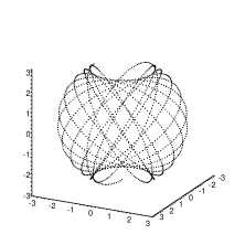
Figure 1: input parameters: $s_{1}^{+}=2+i$, $s_{1}^{-}=2-i$, $s_{1}^{3}=-2$, $s_{2}^{+}=50+40i$, $s_{2}^{-}=50-40i$, $s_{2}^{3}=70$, $\lambda_{1}=\pi/110$, $\lambda_{2}=7\pi/3$, $\lambda_{0}=0.1$, $\mu=-0.002i$

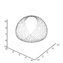
Figure 2: input parameters: $s_{1}^{+}=0.2+10i$, $s_{1}^{-}=0.2-10i$, $s_{1}^{3}=-1$, $s_{2}^{+}=10-30i$, $s_{2}^{-}=10+30i$, $s_{2}^{3}=100$, $\lambda_{1}=\pi$, $\lambda_{2}=7\pi/3$, $\lambda_{0}=0.1$, $\mu=-0.004i$

The figures report an example of iteration of the map (48a), (48b), (48c). For simplicity we take $N=2$. The computations shows the first $1500$ iterations: the plotted variables are the physical ones $(s_{1}^{x},s_{1}^{y},s_{1}^{z})$. Only one of the two spins is shown, namely that labeled by the subscript “1”. The figures are obtained by a ™Maple  code.

References

-
[1]
M.Adler, On the Bäcklund Transformation for the Gel’fand Dickey Equations,
Commun. Math. Phys.80, 517-527, (1981);
M. Adler and P. van Moerbeke: Birkhoff Strata, Bäcklund Transformations, and Regularization of Isospectral Operators, Adv. in Math., 108, 140-204, (1994);
M. Adler and P. van Moerbeke: Toda-Darboux Maps and Vertex Operators, International Mathematics Research Notices, 489-511, 1998. - [2] A.V. Bäcklund, Einiges über Curven und Flächen Transformationen, Lunds Univ. Arsskr., 10 (1874), 1-12.
- [3] L. Bianchi, Ricerche sulle superficie elicoidali e sulle superficie a curvatura costante, Ann. Sc. Norm. Super. Pisa Cl. Sci. (1), 2 (1879), 285-341.
- [4] O. Babelon, D. Bernard, M. Talon, Introduction to Classical Integrable Systems, Cambridge Monographs on Mathematical Physics, (2003)
- [5] L.D. Faddeev, L.A. Takhtajan, Hamiltonian methods in the theory of solitons, Springer-Verlag, 1987.
- [6] G. Falqui, F. Musso, Gaudin models and bending flows: a geometrical point of view, (2003) J. Phys. A, Math. Gen., 36, 11655.
- [7] K. Hikami, Separation of variables in the BC-type Gaudin magnet, J. Phys. A: Math. Gen. , 28 4053-4061 (1995)
- [8] A.N. Hone, V.B. Kuznetsov, O. Ragnisco, Bäcklund transformations for the sl(2) Gaudin magnet, J. Phys. A: Math. Gen., 34, 2477-2490, (2001)
- [9] V.B. Kuznetsov, P. Vanhaecke, Bäcklund transformations for finite-dimensional integrable systems: a geometric approach, J. Geom. Phys. 806, 1-40 (2002)
- [10] V.B. Kuznetsov, E.K. Sklyanin, On Bäcklund tranformations for many-body systems, J. Phys. A: Math. Gen., 31, 2241-2251, (1998), solv-int/9711010
- [11] V.B. Kuznetsov, M. Petrera, O. Ragnisco, Separation of variables and Bäcklund transformations for the symmetric Lagrange top, J. Phys . A: Math. Gen., 37, 8495-8512, (2004).
-
[12]
D.Levi, Nonlinear differential difference equations as Bäcklund transformations, Journal of Physics A: Math.Gen. 14 (1981) pp.1083-1098;
D.Levi, On a new Darboux transformation for the construction of exact solutions of the Schroedinger equation, Inverse Problems 4 (1988) pp.165-172. - [13] F. Musso, M. Petrera, O. Ragnisco, Algebraic extension of Gaudin models, J. Nonlinear Math. Phys., 12, suppl. 1, 482-498, (2005).
- [14] F. Musso, M. Petrera, O. Ragnisco, G. Satta, Bäcklund transformations for the rational Lagrange chain, J. Nonlinear Math. Phys., 12, suppl. 2, 240-252, (2005).
- [15] F.W. Nijhoff, Discrete Dubrovin Equations and separation of Variables for Discrete Systems, in Chaos, Solitons and Fractals, 11, 19-28, Eds. I. Antoniou and F. Lambert, Pergamon Elsevier Science, (2000).
- [16] O. Ragnisco, Dynamical r-matrices for integrable maps, Phys. Lett. A, 198, 4, 295-305, (1995).
-
[17]
O. Ragnisco and Y.B. Suris, On the r-matrix structure of the Neumann system
and its discretizations, in: Algebraic Aspects of Integrable Systems: in
Memory of Irene Dorfman, Birkhäuser, 285-300, (1996);
O. Ragnisco and Y.B. Suris, Integrable discretizations of the spin Ruijsenaars-Schneider models, J. Math. Phys., 38, 4680-4691, (1997) O. Ragnisco and Y.B. Suris, What is the Relativistic Volterra Lattice?, Comm. Math Phys., 200, 2, 445-485, (1999) - [18] O. Ragnisco, F. Zullo, Bäcklund transformations for the Trigonometric Gaudin Magnet, Sigma, 6, 012, 6 pages, (2010).
-
[19]
C. Rogers, Bäcklund Transformations in Soliton Theory: A Survey of Results, in Nonlinear Science: Theory and Applications, Manchester University Press,
97-130, (1990) (Ed. A Fordy);
C. Rogers and W.F. Shadwick, Bäcklund Transformations and Their Applications, Academic Press, New York (1982). - [20] E.K. Sklyanin, Canonicity of Bäcklund transformation: r-Matrix Approach. I, L.D. Faddeev’s Seminar on Mathematical Physics., 277-282, Amer. Math. Soc. Transl.: Ser 2, 201, Amer. Math. Soc., Providence, RI, (2000)
- [21] E. K. Sklyanin, Canonicity of Bäcklund tranformations: r-Matrix Approach.II, Proc. of the Steklov Institute of Mathematics, 226, 121-126, (1999).
- [22] E. K. Sklyanin, Separation of variables. New Trends. Prog. Theor. Phys. Suppl., 118, 35-60, (1995)
- [23] Y. B. Suris, New integrable systems related to the relativistic Toda lattice, J. Phys. A, 30, 1745-1761, (1997)
- [24] Y. B. Suris, The Problem of Integrable Discretization: Hamiltonian Approach, Progress in Mathematics, vol. 219, Birkhäuser, Basel, (2003)
-
[25]
A.P.Veselov, Integrable Maps, Russian Mathematical Surveys 46,
1-51 (1991);
A.P. Veselov, What is an integrable mapping? in What is integrability?, Editor V.E. Zakharov, Springer-Verlag, 251-272, (1991);
A.P. Veselov, Growth and integrability in the dynamics of mappings, Comm. Math. Phys., 145, 181-193, (1992). - [26] M.A. Semenov-Tian-Shansky, Quantum and Classical Integrable Systems Integrability of Nonlinear Systems, vol. 638, Springer Berlin, Heidelberg, (2004).q-alg/9703023.
- [27] S. Wojciechowski, The analogue of the Bäcklund transformation for integrable many-body systems, J. Phys. A: Math. Gen., 15, L653-657, (1982); Corrigendum 16, 671, (1983).