Precision Measurements
of the Top Quark Mass

Frank Fiedler

Ludwig-Maximilians-Universität München

Habilitation thesis

28 February 2007

The experimental status of measurements of the top quark mass is reviewed. After an introduction to the definition of the top quark mass and the production and decay of top quarks, an in-depth comparison of the analysis techniques used in top quark mass measurements is presented, and the systematic uncertainties on the top quark mass are discussed in detail. This allows the reader to understand the experimental issues in the measurements, their limitations, and potential future improvements, and to comprehend the inputs to and formation of the current world average value of the top quark mass. Its interpretation within the frameworks of the Standard Model and of models beyond it are presented. Finally, future prospects for measurements of the top quark mass and their impact on our understanding of particle physics are outlined.

Für Grit, Lukas und Julia

1 Introduction

The top quark is the heaviest known elementary particle. While it has not yet been possible to answer the question why its mass is so large, the precise measurements of the top quark mass that have become available since its discovery have already greatly improved constraints on our picture of nature; for example they have made predictions of the mass of the as yet undiscovered Higgs boson possible. This report first defines the top quark mass and then describes in detail the techniques used to measure it. This is followed by a description of the systematic uncertainties. The current world average value of the top quark mass is presented, and the constraints it provides on elementary particle physics models are shown. Finally, potential future improvements of the precision on the top quark mass are outlined.

Of all known elementary fermions, the top quark has by far the largest mass. This renders the top quark unique from a theoretical standpoint: The top quark Yukawa coupling is close to unity, which may be a hint that the top quark mass is related with electroweak symmetry breaking. Via loop contributions, the masses of the $W$ boson, the top quark, and the yet undiscovered Higgs boson are interrelated so that the Higgs mass (which is not predicted in the Standard Model of elementary particle physics) may be constrained from precise measurements of the $W$ boson and top quark masses [1, 2]. Experimentally, on the other hand, the top quark is unique as it is the only quark that does not hadronize because its lifetime is too short [3]; it is therefore possible to directly measure the properties of the quark instead of a hadron containing the quark of interest.

Long before the discovery of the top quark, its existence as the up-type partner of the bottom quark had been postulated within the Standard Model, and its mass could be predicted from precision measurements of electroweak observables. Currently, indirect constraints within the Standard Model yield a top quark mass value of $m_{t}=178\,^{+12}_{\phantom{0}-9}\,\,\mathrm{Ge\kern-1.00006ptV}$ [2]. The top quark was finally discovered [4] by the CDF and D0 experiments in proton-antiproton collisions at the Fermilab Tevatron Collider. Since then, measurements of the top quark mass have been performed both during Run I of the Tevatron in the 1990s at a proton-antiproton center-of-mass energy of $\sqrt{s}=1.8\,\,\mathrm{Te\kern-1.00006ptV}$ [5] and during the ongoing Run II at an increased center-of-mass energy of $1.96\,\,\mathrm{Te\kern-1.00006ptV}$ and with larger data sets [6, 7, 8]. Their average value of $m_{t}=171.4\pm 2.1\,\,\mathrm{Ge\kern-1.00006ptV}$ [9] is in striking agreement with the indirect prediction, thus supporting the Standard Model as the theory of nature. Innovative measurement techniques have made this precision possible, which already surpasses the original expectations for Tevatron Run II [10]. Within the Standard Model, a value of the Higgs boson mass close to the current lower exclusion limit is favored [2].

The Tevatron experiments have performed many more measurements of top quarks. The total cross section for top-antitop pair production [11, 12] is consistent with the predictions from QCD [13], using the above top quark mass as input. No evidence for effects beyond those predicted in the Standard Model has been found in production and decay of top quarks [14, 15, 16]. A recent review of top quark measurements can be found in [17].

To date, the Tevatron Collider still provides the only possibility to produce top quarks. In the near future, the LHC proton-proton collider will start operation, which is expected to provide much larger samples of top quark events. While the measurement of the top quark mass will be subject to very similar systematic uncertainties, it can be assumed that the large data samples will allow for a further reduction of the error. However, only a linear $e^{+}e^{-}$ collider scanning the $t\bar{t}$ production threshold will allow for an order of magnitude improvement of the precision.

This paper provides an overview of current measurements of the top quark mass at hadron colliders, focusing on the Tevatron Run II results. The purpose of this document is twofold:

• to review the current status of top quark mass measurements, compare the assumptions made in the various analyses, discuss the limiting systematic uncertainties together with potential future improvements, and to give an overview of the interpretation of the measurements; and

• to provide a detailed description of the measurement techniques developed and used so far for the measurement of the top quark mass, not only to complement the information on the physics results, but also as a reference for the development of future measurements (of the top quark or other particles).

The general structure of the paper is as follows: Section 2 gives a brief summary of definitions of the top quark mass and discusses the relevance of measurements of the top quark mass for elementary particle physics. Section 3 then outlines the production mechanisms for top quarks at hadron colliders and the event characteristics. The steps needed to obtain a set of data events with which to measure the top quark mass are described in Sections 4 (reconstruction of top quark events) and 5 (detector calibration).

An overview of the different techniques (template, Matrix Element, and Ideogram methods) to determine the top quark mass from such a set of calibrated data events is given in Section 6. The principle of template based measurements and examples using different event topologies are discussed in Section 7. Section 8 gives an in-depth description of the Matrix Element method, and the Ideogram method is described in Section 9. The fitting procedure to determine the top quark mass is discussed in Section 10.

The current world average of the top quark mass is already dominated by systematic uncertainties. The different sources of systematic uncertainties and the estimation of the size of the corresponding effects are discussed in Section 11. Section 12 then summarizes the current knowledge of the top quark mass and the interpretation of these results and outlines possible future developments. Section 13 summarizes and concludes the paper.

2 Definition and Relevance of the Top Quark Mass

The definition of the mass of a particle may seem trivial. However, when used in conjunction with a quark it is in fact by no means obvious how “mass” should best be defined. This section introduces different possible definitions and states in general terms which kind of measurement determines which mass. The section then outlines how the precise knowledge of the top quark mass improves our understanding of elementary particles and the description of their interactions within the Standard Model of particle physics.

2.1 Definitions of the Top Quark Mass and Measurement Concepts

In general, “the” mass $m$ of a particle is only defined within a theory or model in which it occurs as a parameter. The mass of a particle can then be determined through a comparison of measurements with the predictions of the theory (the validity of the mass value obtained is then restricted to this particular theory). While it is straightforward to find a suitable definition of the mass of a color-neutral particle, there are several possibilities for defining the mass of a (color-charged) quark. This section illustrates the underlying concepts and defines how the word mass is used in conjunction with the top quark in the remainder of this report. See Reference [3] for more detailed reviews of Quantum Chromodynamics (QCD), quark masses, and top quark physics.

For each quark, a mass parameter is introduced in the QCD Lagrangian. (In the Standard Model, the value of this parameter is proportional to the Yukawa coupling of the quark to the Higgs boson.) The value depends on the renormalization scheme and the renormalization scale $\mu$. At high energies, the QCD coupling constant $\alpha_{s}$ is small, and observables are typically calculated in perturbation theory, commonly applying the $\overline{\rm MS}$ renormalization scheme. (The $\overline{\rm MS}$ scheme is used by the Particle Data Group to report all quark masses except the top quark mass.)

For an observable (i.e., non-colored) particle, the position of the pole in the propagator defines the mass. In perturbative QCD, this pole mass can also be used as a definition of quark masses. However, the pole mass cannot be used to arbitrarily high accuracy: Because of confinement (i.e., because of non-perturbative effects in QCD), the full quark propagator does not have a pole. This is true even for the top quark which does not hadronize before decaying. The general argument is presented in a very intuitive way in Reference [18]. The relation between the pole mass and $\overline{\rm MS}$ mass is known to three loops, see [3] and references therein, but there necessarily remains an uncertainty of order $\Lambda_{\rm QCD}$ in the pole mass [18].

Different definitions of the pole mass are used. An unstable particle can generally be described by a Breit-Wigner resonance [19]

$$f(s)\sim\frac{s}{\pi}\,\frac{\tilde{m}\tilde{\Gamma}}{(s-\tilde{m}^{2})^{2}+(\tilde{m}\tilde{\Gamma})^{2}}\ ,$$ (1)

where $s=p^{2}$ is the squared four-momentum of one particle, and the properties of the resonance are described by a constant width $\tilde{\Gamma}$ and the corresponding (pole) mass $\tilde{m}$. It is possible to absorb higher-order corrections into the pole mass definition. For example, for the experimental determination of the $Z$ boson mass an $s$-dependent width is used to describe the resonance, with the term $(\tilde{m}\tilde{\Gamma})$ replaced by $(s\Gamma/m)$. To accomodate the same experimental data, different numerical values of the mass parameter are needed in the two approaches; for the $Z$ boson the relation between the two parameter values is given by [2]

$$m_{Z}=\tilde{m}_{Z}\sqrt{1+\frac{\tilde{\Gamma}_{Z}^{2}}{\tilde{m}_{Z}^{2}}}\approx\tilde{m}_{Z}+34.20\,\,\mathrm{Me\kern-1.00006ptV}\ .$$ (2)

Similarly, different definitions are possible for the top quark mass. Measurements of the top quark mass at a hadron collider rely on comparisons of the data with simulated events, and thus it is important to state the definition adopted in the simulation which is used in the measurement. The two simulation programs used most commonly in current measurements are alpgen [20], which uses fixed widths in propagators, and pythia [19], where a factor $(1-2.5\,\alpha_{s}(s)/\pi)$ is included for top quarks to approximate loop corrections. The energy dependence of $\alpha_{s}$ in principle introduces a difference between the two definitions; this is however negligible compared to the intrinsic uncertainty of order $\Lambda_{\rm QCD}$.

To determine the top quark mass defined in any given scheme, one has to find observables measurements of which can be compared to theory predictions which in turn depend on this top quark mass. In practice, there are three fundamentally different approaches:

• Indirect constraints from electroweak measurements: Even before the first direct observation of top quarks, indirect constraints were obtained from fits of the Standard Model prediction as a function of the top quark mass to precision measurements of electroweak observables [1, 2]. This method of course has the drawback that it is not an actual discovery of the top quark, and that the mass value is only valid within the Standard Model (or in other theories whose predictions do not significantly differ from those of the Standard Model).

• Reconstruction of top quark decay products: Today and in the near future, top quarks are and will be produced at the hadron colliders Tevatron and LHC, allowing for a direct measurement of the top quark mass from the reconstructed decay products. The momenta of the decay products are related according to

  $$m_{t}(i)^{2}=p_{t}(i)^{2}=\left(\sum_{j}p_{j}(i)\right)^{2}\ ,$$ (3)

  where $p$ denotes the 4-momentum of a particle and the sum is over all decay products $j$ of the top quark $t$ in a specific event $i$. A measurement based on the momenta of the decay products thus ideally corresponds to a measurement of the pole mass since the squared sum of four-momenta as given in Equation (3) enters in the denominator

  $${p_{t}^{2}-m_{t}^{2}+im_{t}\Gamma_{t}}$$ (4)

  of the propagator term. Individual measurements differ in how an observable that is related with the top quark mass is constructed from the measured decay products, and the situation is more complicated for measurements relying on complex techniques like the Matrix Element or Ideogram methods discussed in Sections 8 and 9. In the most precise measurements in the $\ell$$+$jets channel, the experimental information comes to a very large extent from the invariant mass of the reconstructed top quark decay products; thus the measured value can be expected to correspond (most closely) to the pole mass, but this issue has not yet been studied in detail.

  In contrast to the other quarks (up, down, charm, strange, and bottom), the top quark decays before forming hadrons [3]. This makes a direct measurement of the top quark mass (instead of a hadron mass) possible; hadronization only affects the decay products of the top quark and leads to jet formation, cf. Section 3.2.

  Top quark mass measurements based on the decay products are valid not only within the Standard Model but in any model which does not introduce significant changes to those features of top quark production and decay that are used in the measurement. However, the results are subject to an intrinsic uncertainty of order $\Lambda_{\rm QCD}$ as mentioned above.

• $t\bar{t}$ threshold scan: In the long-term future, it will be desirable to determine the top quark mass based on a definition that is not subject to the uncertainty on the pole mass, even though the current combined experimental uncertainty is almost a magnitude larger. The best-known example is the measurement of the cross section for top-antitop pair production near threshold at a future $e^{+}e^{-}$ collider. This experimentally very clean measurement could be related to theory predictions that are calculated as a function of a top quark mass parameter that can be translated into the $\overline{\rm MS}$ mass with much smaller uncertainty [21]. The principle of the measurement is analogous to the determination of the $W$ boson mass from the measurement of the $WW$ production cross section at threshold at LEP2.

This report focuses on the techniques, current results, and prospects of top quark mass measurements at the Tevatron, where the mass is reconstructed from the properties of the decay products. Consequently, the pole mass definition is implicitly assumed throughout the remainder of this report unless noted otherwise. This is consistent with the conventions of the Tevatron Electroweak Working Group [9] and the Particle Data Group [3].

2.2 Relevance of the Top Quark Mass within the Standard Model

In perturbation theory, predictions for observables receive contributions from loop diagrams, where particles contribute even if they are too massive to be produced on shell. The size of these corrections to leading-order predictions depends on the values of the masses of the particles in the loops. Of particular importance for Standard Model fits is the dependence of the $W$ boson mass on the top quark and Higgs boson masses. The lowest-order diagram leading to the dependence on the top quark mass is shown in Figure 1(a), those resulting in the Higgs mass dependence in Figures 1(b) and (c). The corrections that arise from these diagrams are quadratic in the top quark mass, but only logarithmic in the Higgs boson mass (yielding a much weaker dependence).

Abbildung 1: Feynman diagrams of loop processes that lead to a dependence of the $W$ boson propagator on (a) the top quark mass and (b, c) the Higgs boson mass.

Since the dependence on the Higgs boson mass is weak, measurements of the $W$ mass (and of other electroweak observables) lead to indirect constraints on the top quark mass. This led to predictions of the mass of the top quark before its actual discovery, as already outlined in Section 2.1. Also, precise measurements of both the $W$ boson and top quark masses result in constraints on the Standard Model Higgs boson mass. In the following sections, the experimental measurements of the top quark mass are discussed in detail. The interpretation of the current results within the Standard Model (and models beyond the Standard Model) is then further discussed in Section 12.2.

3 Top Quark Production and Decay at Hadron Colliders

Top quarks can be studied best when produced on shell in a collider experiment. This is currently only possible at the Fermilab Tevatron proton-antiproton collider near Chicago. In the near future, the LHC proton-proton collider at CERN near Geneva will produce large numbers of top quarks. This section describes the properties of events produced in reactions involving top quark decays.

In this section, the mechanisms for top quark production in hadron collisions ($p\bar{p}$ or $pp$) are described. Events containing a $t\bar{t}$ pair are used to measure the top quark mass, and thus the different topologies of these events, which depend on the top quark decays, are discussed. The relevant background processes are also described.

3.1 Top Quark Production

Because of the large top quark mass, high energies are required to produce top quarks, and the production processes (including those proceeding via the strong interaction) can be described in perturbation theory. The internal structure of the colliding hadrons is resolved, and top quarks are thus produced in a hard-scattering process of two constituent partons (quarks/antiquarks or gluons) inside the hadrons. The description of the reaction factorizes into the modeling of the constituents of the incoming hadrons, of the hard-scattering process yielding the top quarks (and also describing their subsequent decay), and of the formation of the observable final-state particles. A schematic illustration of this factorization scheme is given in Figure 2.

Abbildung 2: Schematic drawing illustrating the concept of factorization. Shown is a collision of two hadrons leading to a hard-scattering process at a scale $Q^{2}$. This hard interaction is initiated by two partons of momenta $x_{1}P_{1}$ and $x_{2}P_{2}$, where $P_{1}$ and $P_{2}$ are the momenta of the colliding hadrons. The partonic cross section $\hat{\sigma}$ of the hard interaction can be calculated perturbatively, based on the renormalization and factorization scales $\mu_{R}^{2}$ and $\mu_{F}^{2}$. The factorization scale is also used to evaluate the parton distribution functions $f_{\rm PDF}$, which parametrize the probabilities to find the partons $a_{1}$ and $a_{2}$ inside the colliding hadrons. If the hard interaction involves the production of top quarks, their decays are included in its description, since the top quark lifetime is so short that no top hadrons are formed. The observable final-state particles are then formed in a hadronization process which again cannot be calculated perturbatively, but is independent of the hard interaction.

To calculate the (differential) cross section for top quark production, a factorization scale $\mu_{F}^{2}$ is introduced to separate the hard-scattering partonic cross section from the modeling of the constituents of the proton/antiproton. The latter is independent of the hard-scattering process, and parton distribution functions (PDFs) $f_{\rm PDF}^{a}(x,\mu_{F}^{2})$ are introduced that describe the probability density to find a parton $a$ (quark or antiquark of given flavor or gluon) with longitudinal momentum fraction $x$ inside a colliding proton. The PDFs cannot be calculated, and are determined in fits to experimental data. As an example, the cteq5l parametrization [22] is shown in Figure 3 for a scale of $\mu_{F}^{2}=(175\,\,\mathrm{Ge\kern-1.00006ptV})^{2}$ (a common choice used in current measurements for the description of top quark production). Even though experimental observables cannot depend on the factorization scale, the PDFs (and the hard-scattering cross section) depend on the value of $\mu_{F}^{2}$ chosen, and an overall dependence remains if calculations are not done to infinite order in perturbation theory. In the following sections, the dependence on the factorization scale is not mentioned explicitly, and the symbol $f_{\rm PDF}^{a}(x)$ is used. To assess the systematic uncertainty related to the choice of factorization scale, experiments compare the results of simulations based on different values for the scale.

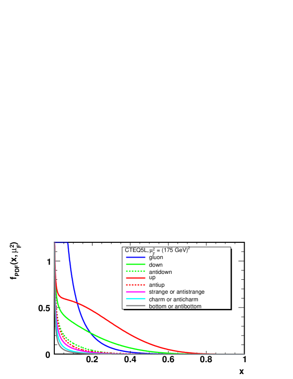
Abbildung 3: The cteq5l parametrization [22] of the distribution functions for different parton species in the proton as a function of the momentum fraction $x$ of the proton carried by the parton, for a factorization scale $\mu_{F}^{2}=(175\,\,\mathrm{Ge\kern-1.00006ptV})^{2}$.

There are two main mechanisms for top quark production at hadron colliders: top-antitop pair production via the strong interaction, and single top production via the electroweak interaction. Single top production has only recently been observed [23], and this process is not (yet) used to measure the top quark mass. Consequently, the emphasis of this section is on $t\bar{t}$ pair production.

The leading-order Feynman diagrams for the hard-scattering process of $t\bar{t}$ production are shown in Figure 4. They apply to both proton-antiproton (Tevatron) and proton-proton (LHC) collisions. When contributions from higher-order diagrams are included, renormalization of divergent quantities becomes necessary. This leads to the introduction of another scale, the renormalization scale $\mu_{R}^{2}$. In practice, the factorization and renormalization scales are often chosen to be equal.

Abbildung 4: Leading-order Feynman diagrams of the hard-scattering processes that lead to $t\bar{t}$ production at a hadron collider: (a) $q\bar{q}\to t\bar{t}$, (b) $gg\to t\bar{t}$.

To obtain the $t\bar{t}$ production cross section in hadron collisions, the partonic cross section $\hat{\sigma}$ must be folded with the appropriate parton distribution functions $f_{\rm PDF}^{a}(x)$, integrated over all possible initial-state parton momenta, and then summed over all contributing initial-state parton species:

$$\sigma(P_{1},P_{2})=\!\sum_{a_{1},a_{2}}\int\!{\rm d}x_{1}{\rm d}x_{2}f_{PDF_{1}}^{a_{1}}\left(x_{1},\mu_{F}^{2}\right)f_{PDF_{2}}^{a_{2}}\left(x_{2},\mu_{F}^{2}\right)\hat{\sigma}\left(x_{1}P_{1},x_{2}P_{2},\alpha_{s}\left(\mu_{F}^{2}\right),\frac{Q^{2}}{\mu_{R}^{2}}\right)\,,$$ (5)

where $P_{1}$ and $P_{2}$ are the momenta of the incoming hadrons, the sum is over all possible combinations of parton species $a_{1}$ and $a_{2}$ that can initiate the hard interaction, and the hard-scattering cross section $\hat{\sigma}$ depends on their momenta, the factorization scale, and the ratio of the scale $Q^{2}$ of the hard interaction and the renormalization scale. Resulting Standard Model predictions for the $t\bar{t}$ production cross section at the Tevatron and LHC are listed in Table 1. At the Tevatron, in proton-antiproton collisions at $\sqrt{s}=1.96\,\,\mathrm{Te\kern-1.00006ptV}$, the quark-antiquark induced process dominates. At the LHC, in proton-proton collisions at $\sqrt{s}=14\,\,\mathrm{Te\kern-1.00006ptV}$, the fraction $x$ of the proton momentum carried by the colliding partons may be much smaller. Because the gluon PDF is much larger at small $x$ than the quark PDFs, the gluon induced process dominates at the LHC. The overall $t\bar{t}$ cross section at the LHC is two orders of magnitude larger than that at the Tevatron.

Channel	Tevatron Run II: $p\bar{p}$ collisions, $\sqrt{s}=1.96\,\,\mathrm{Te\kern-1.00006ptV}$	LHC: $pp$ collisions, $\sqrt{s}=14\,\,\mathrm{Te\kern-1.00006ptV}$
$t\bar{t}$ pair production	$5.8\enspace\hskip 4.30554pt{\text{-}}\hskip 4.30554pt7.4\enspace\,{\rm pb}$ [13]	$830\phantom{.0}\hskip 3.44444pt^{+50\phantom{.0}}_{-40\phantom{.0}}$	${\rm pb}$ [24]
single top, s-channel single antitop, s-channel	$0.98\pm 0.04\,{\rm pb}$ [25]	$\enspace\enspace 7.2\hskip 3.44444pt^{+\phantom{0}0.6}_{-\phantom{0}0.5}$ $\enspace\enspace 4.0\hskip 3.44444pt^{+\phantom{0}0.1}_{-\phantom{0}0.2}$	${\rm pb}$ [26] ${\rm pb}$ [26]
single top, t-channel single antitop, t-channel	$2.2\enspace\pm 0.1\enspace\,{\rm pb}$ [25]	$146\phantom{.0}\pm 5\phantom{.0}$ $\enspace 89\phantom{.0}\pm 4\phantom{.0}$	${\rm pb}$ [26] ${\rm pb}$ [26]
single top+antitop, $W$+$t$ production	$0.26\pm 0.06\,{\rm pb}$ [25]	$\enspace 82\phantom{.0}\pm 8\phantom{.0}$	${\rm pb}$ [26]

Tabelle 1: Predicted top quark production cross sections for various processes at the Tevatron and LHC. The predictions are at next-to-leading order, including threshold corrections from soft gluons. All values are quoted for an assumed top quark mass of $175\,\,\mathrm{Ge\kern-1.00006ptV}$. For the dependence of the cross sections on the top quark mass hypothesis see Figure 43 ($t\bar{t}$ production) and References [25, 26] (single top/antitop production). The range of $t\bar{t}$ cross sections quoted for the Tevatron includes PDF uncertainties (which have been found to be dominant by studying the variations of the CTEQ6 [27] and MRST [28] parametrizations) while the LHC uncertainty is only based on a variation of the renormalization scale. At the Tevatron, the relative contributions of $q\bar{q}$ and $gg$ induced process are roughly $85\%$ and $15\%$; at the LHC these numbers are about $10\%$ and $90\%$, respectively. Wherever the cross sections for single top and antitop production are equal, the sum of the cross sections for both processes is listed. This is the case for single top/antitop production at the Tevatron because it is a proton-antiproton collider. The cross sections for production of a $W$ boson in association with a top or antitop quark are equal also at the LHC because the $b$ and $\overline{b}$ PDFs are equal. The single top cross sections quoted are similar to the next-to-leading order values published in [29].

Production of single top quarks via the electroweak interaction is expected to proceed via three different channels. Predictions for the Standard Model cross sections are given in Table 1, and Figure 5 shows the leading-order diagrams for the three processes. The remainder of this report focuses on $t\bar{t}$ pair production.

Abbildung 5: Leading-order Feynman diagrams of the hard-scattering processes that lead to single top production at a hadron collider: (a) s-channel, (b) t-channel, (c) W+t associated production.

3.2 Top Quark Decay and Event Topologies

In the Standard Model, top quarks decay almost exclusively to a $b$ quark and a $W$ boson [3, 30], and the top quark decay width being much larger than $\Lambda_{\rm QCD}$, no top quark hadronization takes place. Therefore, the event topology of a $t\bar{t}$ event is determined by the decays of the two $W$ bosons. The $b$ quarks and quarks from hadronic $W$ decays hadronize and are reconstructed as jets in the detector. The presence of final-state neutrinos is signalled by missing transverse energy $E\kern-6.00006pt/_{T}$, defined as the magnitude of the transverse momentum vector $\vec{p}\kern-4.49997pt/_{T}$ needed to balance the event in the plane perpendicular to the beam direction.

Commonly, the event topologies are classified as dilepton, lepton+jets ($\ell$$+$jets), and all-jets topologies. These three categories exclude events with one or more tauonic $W$ decays, which are more difficult to reconstruct and provide less mass information than corresponding events with electronic or muonic $W$ decays because of the additional neutrinos from $\tau$ decays. In this report, the word “lepton” always refers to an electron or muon unless otherwise mentioned.

In the following, the characteristics of the topologies used for top quark mass measurements are discussed, the main backgrounds are listed, and the consequences for measurements of the top quark mass are mentioned. The relative abundance of events in the various topologies is shown schematically in Figure 6.

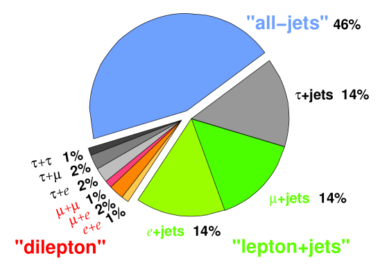
Abbildung 6: Relative abundance of the $t\bar{t}$ event topologies, calculated from the $W$ branching fractions listed in Reference [3]. The figure has been taken from [31], and the values have been updated. Note the rounding errors; the total “dilepton” and “lepton+jets” branching fractions are about $5\%$ and $29\%$, respectively.

• Dilepton Events: In about $5\%$ of $t\bar{t}$ events, both $W$ bosons decay into an electron or a muon plus the corresponding neutrino. These so-called dilepton events are characterized by two oppositely charged isolated energetic leptons, two energetic $b$ jets, and missing transverse energy due to the two neutrinos from the $W$ decay.

  Because of the two charged leptons, these events are relatively easy to select. The largest physics background is from production of a $Z$ boson (decaying to $e^{+}e^{-}$ or $\mu^{+}\mu^{-}$) in association with two jets. This background affects only the dielectron and dimuon channels and can be reduced by requiring that the invariant dilepton mass be inconsistent with the $Z$ mass. Correspondingly, the $e\mu$ channel is very clean; here, the main physics background is from $Z\to\tau^{+}\tau^{-}$ decays where the $Z$ boson is produced in association with two jets. Instrumental background where a hadronic jet with a leading $\pi^{0}\to\gamma\gamma$ decay is misidentified as an isolated electron is also important at the Tevatron experiments.

  In spite of the small backgrounds the statistical information on the top quark mass that can be extracted per dilepton event is limited because the event kinematics is underconstrained when the top quark mass is treated as an unknown. The 4-momenta of the 6 final-state particles are fully specified by 24 quantities; the 6 masses are known, and the 3-momenta of four particles (the two jets and the two charged leptons) are measured in the detector. Additional constraints can be obtained by assuming transverse momentum balance of the event (2), the known masses of the $W$ bosons (2), and by imposing equal top and antitop quark masses (1 constraint). This leads to 23 quantites that are known, measured, or can be assumed. The event kinematics could therefore only be solved if the value of the top quark mass itself were also assumed. Consequently, to measure the top quark mass, additional information is used, e.g. the relative probabilities for different configurations of final-state particle momenta.

• Lepton+Jets Events: Those $29\%$ $t\bar{t}$ events with one $W\to e\nu$ or $W\to\mu\nu$ and one hadronic $W$ boson decay are called lepton+jets events. They contain one energetic isolated lepton, four energetic jets (two of which are $b$ jets), and missing transverse energy.

  The main background is from events where a leptonically decaying $W$ is produced in association with four jets. Multijet background where one jet mimicks an isolated electron also plays a role.

  In lepton+jets events, the transverse momentum components of the one neutrino can be obtained from the missing transverse momentum, and the event kinematics is overconstrained when assuming equal masses of the top and antitop quarks and invariant $\ell\nu$ and $q\bar{q}^{\prime}$ masses equal to the $W$ boson mass. The measurement of the top quark mass is however complicated by the fact that the association of measured jets with final-state quarks is not known. The number of possible combinations and also the background can be reduced when $b$ jets are identified ($b$-tagging).

  Today, the lepton+jets topology yields the most precise top quark mass measurements.

• All-Jets Events: In $46\%$ of $t\bar{t}$ events both $W$ bosons decay hadronically, yielding 6 energetic jets, no charged leptons, and no significant missing transverse energy.

  The background from multijet production is large (and cannot easily be modeled with Monte Carlo generators). It can be reduced with $b$-tagging information, which is also important to reduce combinatorics in the jet-quark assignment.

The aim is to measure the top quark mass in all three categories in order to cross-check the measurements and to search for signs of effects beyond the Standard Model. The above picture could be changed if non-Standard Model particles with masses below the top quark mass exist. An example are top quark decays to a $b$ quark and a charged Higgs boson in supersymmetric models: Depending on the parameters of the model, charged Higgs decays could alter the relative numbers of events in the different $t\bar{t}$ event topologies or lead to events with extra jets in the final state [30].

4 Event Reconstruction and Simulation

The previous section gave an overview of the production of top quarks at hadron colliders and of the topologies of top quark events. This section describes how top quark events are reconstructed in the detector. It also briefly introduces the simulation of events.

To measure the top quark mass, $t\bar{t}$ events must first be identified online as potentially interesting and saved for further analysis. The $t\bar{t}$ decay products (charged lepton(s), jets, and missing transverse energy from the neutrino(s)) are then reconstructed. The top quark mass is obtained from the energies/momenta and directions of the decay products measured in the detector.

A brief overview of the CDF and D0 detectors at the Tevatron is given in Section 4.1. In Section 4.2, the trigger requirements used at CDF and D0 for the different $t\bar{t}$ event topologies are presented, and Section 4.3 briefly discusses the reconstruction and selection of electrons, muons, and jets and the identification of $b$ quark jets. Section 4.6 describes the simulation of events used to verify and calibrate the techniques for the top quark mass measurements. The detector calibration and the determination of the detector resolution are described in Section 5.

4.1 The CDF and D0 Detectors

The CDF and D0 Run II detectors are described in detail elsewhere [32, 33]. Both detectors have the standard cylindrical setup of a general-purpose collider detector. From the interaction region in the center of the detector, particles first traverse the tracking detector surrounding the beam pipe. Here, the trajectories of charged particles and their transverse momenta are measured. The tracking detector can be subdivided into a silicon microvertex detector needed for precise primary and secondary vertex reconstruction and a larger-volume tracking chamber providing the lever arm to reconstruct the transverse momentum from the curvature of the track in a solenoidal magnetic field. The calorimeters are used to measure the energy and direction of electrons, photons, and hadronic jets. They are adapted to the different properties of both electromagnetic and hadronic showers. Finally, the calorimeters are surrounded by tracking detectors which serve to identify muons, which are the only charged particles that traverse the calorimeter without being absorbed. Schematic drawings of both CDF and D0 are shown in Figure 7. Both experiments employ a three-layer trigger system that allows for an online selection of events for further analysis. All subdetectors, their readout electronics, and the trigger system are adapted to the Tevatron bunch crossing frequency of $1/(396\,{\rm ns})$.

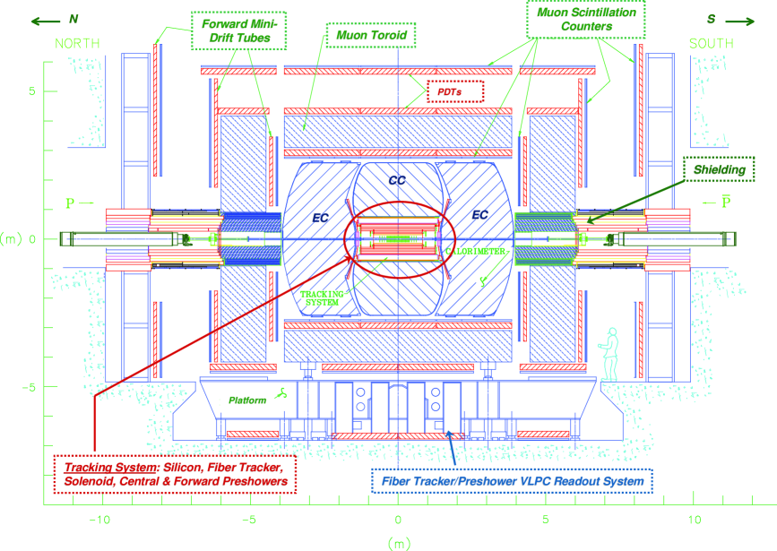
Abbildung 7: Schematic drawings of the CDF [34] (top) and D0 [35] (bottom) detectors during Tevatron Run II.

As far as details of some of the subdetectors are concerned, CDF and D0 differ significantly. However, the general functionality is very similar, and both experiments reconstruct charged leptons, hadronic jets, secondary decay vertices, and missing transverse energy which are then used to select $t\bar{t}$ candidate events and measure the top quark mass. The experiments use a coordinate system centered at the interaction point with the $z$ axis along the beam pipe. Directions are expressed in terms of the azimuthal angle $\phi$ around the beam pipe and the pseudorapidity $\eta=-\ln\left(\tan(\theta/2)\right)$, where $\theta$ is the polar angle relative to the $z$ axis.

Of the integrated luminosity of more than $2\,\,\rm fb^{-1}$ delivered to each of CDF and D0, up to $1\,\,\rm fb^{-1}$ has been used so far in top quark mass measurements. In comparison, Run I measurements were based on integrated luminosities of the order of $100\,\,\rm pb^{-1}$. A total integrated luminosity per experiment of $4-9\,\,\rm fb^{-1}$ is expected until the end of Run II of the Tevatron.

4.2 Trigger Strategies

Triggering $t\bar{t}$ event candidates that involve at least one leptonic $W$ decay is relatively straightforward because of the presence of an isolated electron or muon with large transverse energy or momentum. The presence of energetic jets can be used as an additional trigger criterion.

To identify dilepton candidate events, both CDF and D0 require the events to be triggered by the presence of a high-$E_{T}$ electron or high-$p_{T}$ muon [36, 37]. While CDF requires one electron or muon, in the D0 analysis two charged leptons in the first-level trigger and one or two (depending on the channel) charged leptons in the high-level triggers are required.

In the $\ell$$+$jets event topology, CDF also relies exclusively on the charged lepton trigger [38]. The D0 experiment requires a charged lepton and a jet, both with large transverse momentum or energy, to be found in the trigger [39].

Triggering $t\bar{t}$ events in the all-jets channel is more difficult because of the large QCD multijet background. The CDF analysis [40] uses a trigger that requires at least four jets and a minimum scalar sum of transverse energies, $H_{T}$, of at least 125 GeV. In the all-jets channel, the D0 experiment has performed a measurement of the $t\bar{t}$ cross section [41], but not yet of the top quark mass.

The characteristics of dilepton and $\ell$$+$jets $t\bar{t}$ events are distinctive, so typical trigger efficiencies are around 90% or above (see for example [42]). In the all-jets channel, the CDF experiment quotes a trigger efficiency of 85% [43]. In general, the trigger requirements and therefore also the efficiencies vary as conditions are adjusted to changing instantaneous luminosity. The efficiencies are measured in the data as outlined in Section 5 as a function of the momenta of reconstructed particles (charged leptons, jets) in the event. The overall probability for a simulated event to pass the trigger conditions is obtained as the weighted average of the trigger efficiencies, taking into account the relative integrated luminosity for which each trigger condition was in use [44]. The trigger efficiency depends on the top quark mass, mainly because of the $p_{T}$ or $E_{T}$ cuts imposed in the trigger, and this effect must be taken into account in the mass measurement.

4.3 Reconstruction and Selection of Top Quark Decay Products

The offline reconstruction of the events selected by the trigger criteria aims at (1) further reducing the backgrounds and (2) reconstructing the momenta of the $t\bar{t}$ decay products as precisely as possible to obtain the maximum information on the top quark mass. In this section, the reconstruction and selection of isolated energetic charged leptons, of energetic jets, and of the missing transverse energy in $t\bar{t}$ event candidates are discussed. Also, the different possibilities for the identification of bottom-quark jets are described.

4.3.1 Charged Lepton Selection

Electrons are identified by a charged particle track pointing at an electromagnetic shower in the calorimeter. Additional criteria are then applied [39, 45]: Background from mis-identified hadrons is reduced based on the ratio of the energy measured in the electromagnetic and hadronic calorimeter, the shower shape, and on the quality of the match between the calorimeter shower and the charged particle track. CDF in addition vetos electrons from photon conversion processes. Non-isolated electrons, e.g. from semielectronic heavy-hadron decays in jets, are rejected by isolation criteria that impose a maximum calorimeter energy in a cone around the electron.

Muons traverse the calorimeter and leave a track both in the central tracking chamber and in the muon chambers. The following criteria are applied to select muons from $W$ decay in $t\bar{t}$ events [39, 45]: Background from mis-identified hadrons is reduced based on the distance between the central track extrapolated to the muon chambers and the muon chamber track. In addition, CDF requires the energy deposit in the calorimeter to be consistent with that of a minimum ionizing particle, and rejects muons with too large a distance of closest approach in the transverse plane, $d_{0}$, to the beam spot. Cosmic ray muons are rejected based on timing information. As for electrons, non-isolated muons, e.g. from semimuonic heavy-hadron decays in jets, are rejected by isolation criteria requiring a maximum calorimeter energy in a cone around the muon not to be exceeded. The D0 experiment in addition imposes a similar isolation criterion based on the transverse momenta of tracks in a cone around the muon direction.

Finally, a fiducial and kinematic selection is applied. To ensure reliable electron reconstruction in the calorimeter, electron candidates must be well within the central or forward calorimeters, excluding the overlap regions around $|\eta|\approx 1$. Some analyses exclude electrons in the forward calorimeter. The pseudorapidity range within which muons can be identified is limited by the acceptance of the tracking chamber. Typically, electrons (muons) are required to have a transverse energy (momentum) larger than a cut value between 15 and 25 GeV, depending on the analysis. Here, the calibrated energy and momentum values are used; the detector calibration is described in Section 5.

4.3.2 Primary Vertex Reconstruction

The position of the primary vertex is needed in order to compute the jet directions and to identify bottom quark jets using secondary vertex information. While the position of the hard interaction in the transverse plane (“beam spot”) is well determined, the interaction region extends over tens of centimeters along the beam line. Tracking information is used to measure the $z$ position of the primary vertex for each event. Since there may be multiple interactions per event, the vertex associated with the $t\bar{t}$ decay has to be identified. This is done based on reconstructed charged lepton information (CDF analyses involving charged leptons), or the vertex most consistent with the $t\bar{t}$ decay is selected among the candidates [46, 44].

4.3.3 Jet Reconstruction and Selection

The final-state quarks in $t\bar{t}$ events are reconstructed as jets, using a cone algorithm [47, 48] with radius $\Delta{\cal R}=\sqrt{(\Delta\eta)^{2}+(\Delta\phi)^{2}}=0.4$ (CDF) or 0.5 (D0). The jet transverse energy is defined using the primary vertex position described in the previous section. The D0 experiment applies cuts to select well-measured jets [39], and both CDF and D0 ensure that calorimeter energy deposited by electron candidates is not used in the jet reconstruction. A minimum number of jets within a fiducial calorimeter volume of typically $|\eta|<2.0$ (CDF, [45]) or $|\eta|<2.5$ (D0, [39]) and with a (calibrated) transverse energy above a cut value of typically 15 or 20 GeV is required. The calibration of the calorimeter energy scale is discussed in Section 5.

4.3.4 Missing Transverse Energy

Neutrinos can only be identified indirectly by the imbalance of the event in the transverse plane. A feature of lepton+jets and dilepton $t\bar{t}$ events is thus significant missing transverse energy $E\kern-6.00006pt/_{T}$. The missing transverse momentum is reconstructed from the vector sum of all calorimeter objects, i.e. using finer granularity than the reconstructed jets and thus taking into account also small additional energy deposits [39, 45]. The missing transverse momentum vector is corrected for the energy scale of jets and for muons in the event. For the selection of lepton+jets events typically a missing transverse energy of $E\kern-6.00006pt/_{T}>20\,\,\mathrm{Ge\kern-1.00006ptV}$ is required; the cut value for dilepton analyses is usually higher.

The unclustered transverse energy $E_{T}^{\rm uncl}$ is defined as the magnitude of the vector sum of transverse energies of all calorimeter objects that are not assigned to a jet or charged lepton.

4.3.5 Identification of Bottom Quark Jets

A $t\bar{t}$ event contains two bottom quark jets, while jets in background events predominantly originate from light quarks or gluons. This is why the signal to background ratio is significantly enhanced after the requirement that at least one of the jets is $b$-tagged. In addition, the number of relevant assignments of reconstructed jets to final-state quarks (jet-parton assignments) can be considerably reduced with $b$-tagging information.

Three different signatures can in principle be used to identify bottom-quark jets:

• The presence of an explicitly reconstructed secondary vertex corresponding to the decay of the bottom-flavored hadron,

• a low probability for all charged particle tracks in the jet to come from the primary event vertex (which again implies the existence of a displaced secondary decay vertex), or

• the presence of a charged lepton within the jet from a semileptonic bottom or charm hadron decay.

To date, for measurements of the top quark mass using $b$ tagging, explicit secondary vertex reconstruction is used, which proceeds as follows [44, 46]. Tracks in the jet passing a $p_{T}$ cut are selected if they have significant impact parameter relative to the primary event vertex. CDF rejects poorly reconstructed tracks based on the hits and the track fit $\chi^{2}$; D0 rejects tracks from $K^{0}_{\rm s}$ and $\Lambda$ decays and requires that the impact parameter of any track used in secondary vertex finding have a positive projection onto the jet axis (negative when determining the mistag efficiency, see below). Jets are called taggable if they contain at least two tracks that pass these criteria. These tracks are used to form secondary vertices; if a vertex is found with a large positive decay length significance $L_{xy}/\sigma(L_{xy})$ ($>3$ for CDF and $>7$ for D0) the jet is called $b$-tagged. The distance $L_{xy}$ in the $xy$ plane between primary and secondary vertex is multiplied by the sign of the cosine of the angle $\phi$ between the vector pointing from the primary to the secondary vertex and the jet momentum vector. While a large positive value of $L_{xy}$ is a sign for a decay of a long-lived particle, the distribution of negative values contains information about the $L_{xy}$ resolution. Jets tagged with negative $L_{xy}$ are used in the determination of the mistag efficiency, i.e. the efficiency with which non-$b$ quark jets are erroneously tagged, see Section 5.3.

4.4 Backgrounds and $t\bar{t}$ Event Selection

Two types of background have to be distinguished: (1) physics background where all final-state particles are produced but in a different reaction; generally these processes will not involve top quarks, but misassignment of top quark events to the wrong event topology also has to be taken into account; and (2) instrumental background, where part of the event is mis-reconstructed. At a hadron collider, instrumental background mainly involves jets that lead to wrongly identified isolated leptons. Together with the backgrounds, a general outline of the event selection for the different $t\bar{t}$ topologies is given below; concrete examples of event selection criteria are described more fully later together with the top quark mass measurements.

4.4.1 Dilepton Events

Physics background in the dilepton channel arises from all processes leading to a final state with two charged leptons of opposite charge and two jets. For the $ee$ and $\mu\mu$ channels, the largest background is from Drell-Yan events containing two additional jets. These events can be efficiently removed by requiring a minimum charged lepton $p_{T}$ (to remove low-mass resonances), inconsistency of the dilepton invariant mass with the $Z$ mass, and significant missing transverse energy. For all dilepton channels, $Z/\gamma^{*}\to\tau\tau$ events with two leptonic $\tau$ decays as well as diboson events (the $WW$ cross section is largest, but $WZ$ events also have to be taken into account) with leptonic $W$ decay remain. For the dilepton channels as well as the other channels, misidentification of $t\bar{t}$ events containing tauonic $W$ decays with subsequent leptonic $\tau$ decay has to be accounted for.

Instrumental background in the dilepton channel arises mainly from events with one leptonic $W$ decay and three jets, one of which is mis-identified as another lepton. Jets can appear as isolated electrons if they contain a leading $\pi^{0}\to\gamma\gamma$ decay, resulting in large electromagnetic energy deposition in the calorimeter, possibly with a track pointing at it from conversion ($\gamma\to e^{+}e^{-}$) of one of the photons, and only little surrounding jet activity. Additional contributions come from semileptonic bottom or charm hadron decays within jets.

Leptons from $\tau$ decays and jets not from top quark decay have mostly small transverse energies. To select $t\bar{t}$ dilepton event candidates, the experiments thus typically require two charged leptons of opposite charge with large $E_{T}$ and spatially isolated from jet activity, two large-$E_{T}$ jets, and significant missing transverse energy. Most of the remaining background can be removed by requiring jets to be $b$-tagged; however, this is often not desirable for small data samples.

4.4.2 Lepton+Jets Events

Leptonic $W$ decays produced in association with jets, which lead to instrumental background for dilepton events, are the main physics background for $t\bar{t}$ events in the $\ell$$+$jets channel. Another physics background is from electroweak single top production with additional jets. Diboson events contribute when in contrast to above, one leptonic $W$ decay occurs together with another hadronic weak boson decay. Background from events with a leptonic $Z$ decay can be removed by rejecting events with more than one isolated energetic charged lepton. Similarly, background from $Z/\gamma^{*}\to\tau\tau$ events arises if one $\tau$ decays leptonically and the other hadronically.

Instrumental background in the $\ell$$+$jets channel is due to QCD multijet events with at least five jets, one of which is mis-identified as a lepton as described above.

Lepton+jets $t\bar{t}$ events are selected by requiring one isolated charged lepton with large $E_{T}$, normally four large-$E_{T}$ jets at least one of which is $b$-tagged (both requirements can be relaxed), and significant missing transverse energy.

4.4.3 All-Jets Events

The overwhelming background in the all-jets channel is from QCD multijet events that contain six or more reconstructed jets. Most of this background does not contain $b$ jets, and the kinematic properties of the jets differ slightly from those of jets in signal events. The selection relies on a combination of $b$ tagging and kinematic criteria. Since the QCD multijet process cannot be reliably simulated and the total background has to be estimated from the data, there is no need to explicitly account for individual subdominant background processes.

4.5 Jet-Parton Assignment

In most analyses, in particular those based on explicit top quark mass reconstruction, the reconstructed jets need to be assigned to the final-state quarks from the $t\bar{t}$ decay to measure the top quark mass. Depending on the $t\bar{t}$ topology, different numbers of possible jet-parton assignments have to be considered; for all-jets events, 90 different assignments have to be distinguished. In $\ell$$+$jets and all-jets events, the number of relevant assignments can be reduced when $b$-tagged jets are present, which are likely to be direct top quark decay products.

A further complication arises when additional jets are present in the event. Since jets from initial-state radiation, from the underlying event (interactions involving the proton or antiproton remnant), or from additional hard interactions in the same beam crossing typically have small transverse energy $E_{T}$, many analyses consider the $n$ highest-$E_{T}$ jets as $t\bar{t}$ decay products, where $n=2,4,6$ in the dilepton, $\ell$$+$jets, and all-jets topologies, respectively.

The issue of jet-parton assignment is further discussed in Sections 7, 8, and 9 together with the individual analyses.

4.6 Simulation

Monte Carlo simulated events are used for several purposes in the analyses:

• to compare measured and simulated distributions in order to check the detector;

• to determine the detector resolution;

• to optimize the selection and determine the fraction of signal events in the selected data sample;

• to calibrate the methods for measuring the top quark mass; and

• to compare the top quark mass uncertainty obtained in the data with the value expected for the measured fraction of signal events.

Simulation programs are based on the factorization scheme (cf. Section 3.1), and in general, separate program libraries can be used to model the hard interaction, additional gluon and photon radiation in the initial and final state, the parton distribution functions, hadronization, decays of unstable particles, and the detector response. Interference between different processes populating the same experimental final state is usually neglected. This is a good approximation since the final-state color, flavor, and spin configurations are in general different: For example, $\ell$$+$jets $t\bar{t}$ production can only interfere with those $W$$+$jets events that contain a $b\bar{b}$ pair and two additional quarks (but no hard gluons) in the final state.

The simulation used so far in the Tevatron analyses is based on leading-order matrix elements to describe the hard process. The Monte Carlo generators pythia [19], herwig [49], or alpgen [20] are used to generate the hard parton-scattering process in $t\bar{t}$ events and background events involving weak vector bosons ($W$$+$jets events; $WW$, $WZ$, and $ZZ$ events; single top production; and Drell-Yan events in association with jets). These generators are interfaced to leading-order parton distribution functions, in general cteq5l [22]. Leading-order calculations of total cross sections have large uncertainties, and where possible, absolute production rates are scaled to accommodate the data, so that only the prediction of relative cross sections is taken from the simulation.

The simulation of the hard-scattering process is interfaced with pythia or herwig to simulate initial- and final-state gluon radiation. Matching procedures have been developed to ensure that the phase space regions covered by hard gluon radiation and by gluon emission included in the matrix element calculations do not overlap. pythia or herwig are also used to model fragmentation and hadronization, and are interfaced with evtgen [50] or qq [51] and tauola [52] to simulate heavy hadron and tau lepton decays. The simulated events are passed through a detailed simulation of the detector response based on geant [53] and are then subjected to the same reconstruction and selection criteria as the data. A detailed general discussion of the event simulation process can be found in [54], and a list of programs used for top quark measurements is given in [55].

Depending on the instantaneous luminosity, it is possible that more than one $p\bar{p}$ or $pp$ collision takes place in one bunch crossing. To simulate this effect, minimum bias events (events with only very loose trigger requirements) are recorded and superimposed on the simulated events. Similarly, pileup of signals from collisions in subsequent bunch crossings is simulated by overlaying events recorded with a random trigger.

Background not involving any leptons from vector boson decay (QCD multijet background) is not modeled using Monte Carlo simulation, but estimated from the data using events with non-isolated leptons [44, 56] and/or little $E\kern-6.00006pt/_{T}$ [57]. An exception is one CDF analysis in the all-jets final state, where alpgen is used to model the multijet background [58].

The reconstructed energies and momenta in the simulation are smeared such that the detector resolution agrees with that of the actual data. The modeling of kinematic distributions in the simulation is then checked. Signal events are generated for various assumed top quark masses in order to calibrate the measurement methods.

5 Detector Calibration

To measure the top quark mass it is not sufficient to merely select $t\bar{t}$ event candidates. An accurate understanding of how the detector responds to the decay products in $t\bar{t}$ events is also indispensable. It is only this second step that allows to relate the properties of the events to the value of the top quark mass. The procedures with which the experiments calibrate the detector response are outlined in this section.

An accurate calibration of the energy/momentum scale and resolution for the reconstructed particles used to measure the top quark mass is crucial. Also, even though the measured top quark mass does not directly depend on the absolute detector efficiency, the dependence of the efficiency on particle energies/momenta and pseudorapidities must be known, too. In this section, the calibration procedures used by the Tevatron experiments are introduced. It is worth noting that usually a large fraction of the analysis work needed in a top quark mass measurement is related to detector calibration.

5.1 Charged Leptons

The reconstruction of electrons and muons can be calibrated using $Z\to e^{+}e^{-}$ and $Z\to\mu^{+}\mu^{-}$ decays. In addition, information from $W\to e\nu$ events, cosmic ray muons, and $c\bar{c}$ and $b\bar{b}$ resonance decays can be used. These events have the advantage that they can be identified with low backgrounds, and that the measurement of one particle or by one detector system can be cross-checked with another. The electromagnetic calorimeter yields the most precise measurement of the energy of energetic electrons, while the central tracking chamber is used to measure the muon (transverse) momentum.

The transverse momentum scale for energetic muons is adjusted such that the reconstructed $Z$ mass reproduces the known value. Additional information on the momentum scale is obtained from the lower-mass resonance decays $J/\psi\to\mu^{+}\mu^{-}$ and $\Upsilon(1S)\to\mu^{+}\mu^{-}$. The reconstructed invariant mass distribution of $Z\to\mu^{+}\mu^{-}$ decays obtained with the CDF experiment is shown in Figure 8(a) [59]. An example of further studies of the momentum scale is given in Figure 9 [60], which shows the $Z\to\mu^{+}\mu^{-}$ mass distribution for D0 data in events where (1) both muons are isolated and (2) one muon fails the isolation criteria, indicating the presence of Bremsstrahlung.

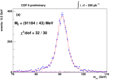
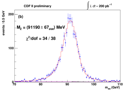
Abbildung 8: Distributions of invariant dilepton masses for (a) $Z\to\mu^{+}\mu^{-}$ and (b) $Z\to e^{+}e^{-}$ decays reconstructed with the CDF detector [59].

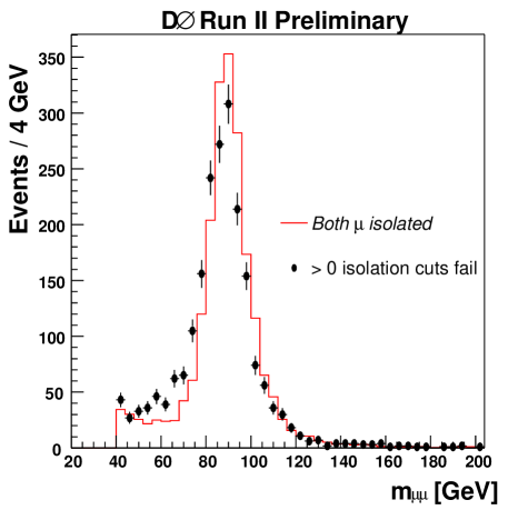
Abbildung 9: Distribution of the invariant $\mu^{+}\mu^{-}$ mass for selected $Z\to\mu^{+}\mu^{-}$ events in the D0 data for isolated muons (histogram) and events where at least one muon does not pass all isolation cuts (points with error bars, scaled to the same number of entries) [60].

The energy scale for energetic electrons is set with the reconstructed $Z\to e^{+}e^{-}$ invariant mass distribution. The distribution obtained by the CDF experiment is shown in Figure 8(b). Additional input is obtained from a comparison of reconstructed electron energy and track momentum in $W\to e\nu$ decays as discussed below. The resulting uncertainties in the calibration of the absolute muon momentum and electron energy scales are negligible for top quark mass measurements (compared with the jet energy scale uncertainties, see below).

The energy/momentum resolution can be studied using $Z\to e^{+}e^{-}$ and $Z\to\mu^{+}\mu^{-}$ events, too. Also, a cosmic ray muon traversing the center of the detector is reconstructed as two muons, and the distribution of the difference between the two reconstructed momenta yields additional information on the momentum resolution. Similarly, since the calorimeter energy measurement is more precise at high energies than the track momentum, a comparison between the two quantities in clean samples of isolated electrons can be made to cross-check the track momentum resolution. Figure 10 shows the results of these studies with CDF data [61].

Abbildung 10: Distribution of the difference in curvature for the two tracks in a CDF cosmic ray event (a), yielding a measurement of the momentum resolution. Distribution of the energy divided by momentum in $W\to e\nu$ events at CDF (b) together with a Gaussian fit in the range $0.8<E/p<1.08$. Electrons with with significant Bremsstrahlung at large $E/p$ are excluded from the fit; their abundance is a measure of the amount of detector material.

The efficiency to reconstruct an electron or muon can be factorized into several contributions: trigger efficiency, tracking efficiency, the efficiency to identify the track as electron or muon, and the efficiency of further criteria like isolation cuts. All individual efficiencies are measured in the data using $Z\to\ell^{+}\ell^{-}$ events (CDF determines the tracking efficiency with $W\to e\nu$ candidate events using calorimeter-only selection criteria), see for example [60, 61, 62]. The concept of the tag-and-probe method in $Z\to\ell^{+}\ell^{-}$ events is visualized in Figure 11: A clean sample of $Z\to\ell^{+}\ell^{-}$ events is obtained using a selection where the criterion under investigation is not applied to one of the leptons. The fraction of selected events where this lepton also passes the additional criterion is then a measure of the efficiency.

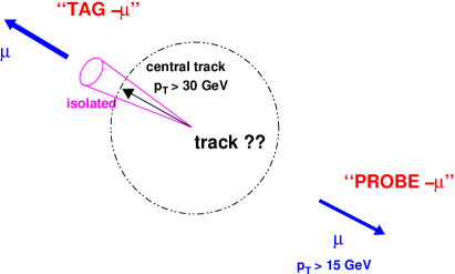
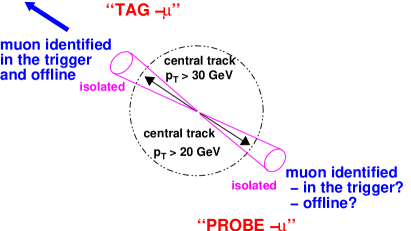
Abbildung 11: Schematic illustration of the tag-and-probe method to measure the tracking efficiency (left) and the efficiency of the charged lepton identification in the trigger and offline [60].

The calibration of top quark mass measurements relies heavily on the quality of the detector simulation. The simulation is tuned (and an additional scaling and smearing is applied where necessary) to reproduce the position and width of the $Z\to\ell^{+}\ell^{-}$ invariant mass peak. This can for example become necessary when the description of the detector material or alignment in the simulation does not fully reproduce reality. Also, the efficiency in the simulation may have to be scaled.

5.2 Hadronic Jets

For the same reasons as outlined above in the section about charged leptons, it is crucial to have a precise knowledge of the jet energy scale and resolution, and to accurately reproduce them in the simulation. In most analyses, the measurement of the top quark mass relies to a large extent on the reconstructed jet energies. However, the energy scale and resolution of jets is more difficult to determine experimentally than that of charged leptons. Therefore, current top quark mass measurements are systematically dominated by the knowledge of the absolute jet energy scale [9], and for a given sample and analysis technique the statistical error on the top quark mass is dominated by the jet energy resolution (see below for a more detailed discussion).

In the following, the determination of the jet energy scale, the relevance of the jet energy resolution, and the agreement between data and Monte Carlo simulation are discussed.

5.2.1 Overall Jet Energy Scale

For the determination of the top quark mass, the momentum vectors of the quarks in the final state are needed. However, the detectors measure particle jets, and their directions and energies are taken as a measure of the quark momentum. While the direction of the initial quark is quite well reproduced by the jet direction, the correspondence between jet and quark energies is more involved. This correspondence is established in two steps:

1. First, the energy of the measured jet is related to the true energy of the particle jet. This step depends on detector effects and on the jet algorithm used.

2. Second, the quark energy is inferred from the particle jet energy. This second step only involves the effects of fragmentation and hadronization and is thus independent of the experimental setup. Depending on the analysis, this relation can be established via Monte Carlo models or via a parametrization with transfer functions.

In this section, the correction procedures applied by the two Tevatron experiments to obtain particle jet energies are outlined; for details, see [63, 64]. The transition to quark energies is regarded as part of each specific top quark mass measurement and is described later in Sections 7-9 together with the individual analyses.

The transition from measured to true particle jet energies requires several corrections:

• Energy Offset $E_{O}$: Before corrections are made, the energy scale for the electromagnetic calorimeter is set such that the $Z\to e^{+}e^{-}$ peak is correctly reproduced, as described in Section 5.1. Contributions from detector noise, energy pile-up from previous bunch crossings, additional interactions in the same bunch crossing (“multiple interactions”), and the underlying event, i.e. reactions of partons in the proton and antiproton other than those that initiated the $p\bar{p}\to t\bar{t}$ process, are then subtracted from the measured jet energy. The correction for this energy offset $E_{O}$ depends on the jet algorithm and parameters (e.g. the cone size), the pseudorapidity, and the instantaneous luminosity. The D0 experiment determines it from energy densities in minimum bias events.

• Calorimeter Response $R$: The second correction concerns the calorimeter response. There is no straightforward way to determine the response with a resonance similar to the procedure applied for electrons and muons based on leptonic $Z$ decays as described in Section 5.1, because hadronic decays of single $W$ or $Z$ bosons cannot be distinguished experimentally from QCD dijet events. (An exception are hadronic $W$ decays in $t\bar{t}$ events, which are discussed below.)

  The response to hadronic jets can therefore only be measured with events where a jet is balanced by another object for which the detector response is known. The D0 experiment uses $\gamma$+jet events, taking the photon energy scale from $Z\to e^{+}e^{-}$ events. In these events, the so-called missing $E_{T}$ projection fraction method allows to measure the calorimeter response from the $p_{T}$ imbalance [64]: For an ideal detector, the photon transverse momentum $p_{T}^{\gamma}$ and the transverse momentum of the hadronic recoil $p_{T}^{\rm had}$ are expected to be balanced. However, before calibration of the calorimeter response an overall transverse momentum imbalance $\vec{p}\kern-4.49997pt/_{T}\neq\vec{0}$ may be observed:

  $$R^{\gamma}\vec{p}_{T}^{\,\gamma}+R^{\rm had}\vec{p}_{T}^{\,\rm had}=-\vec{p}\kern-4.49997pt/_{T}\ .$$ (6)

  The missing transverse momentum vector is corrected for the electromagnetic calorimeter response $R^{\gamma}$ determined from $Z\to e^{+}e^{-}$ events. After that, the hadronic response is obtained as

  $$R^{\rm had}=1+\frac{\vec{p}\kern-4.49997pt/_{T}^{\,\,\rm corr}\cdot\vec{p}_{T}^{\,\gamma}}{\left(\vec{p}_{T}^{\,\gamma}\right)^{2}}\ .$$ (7)

  In events with one photon and exactly one jet, the jet response can be identified with the hadronic response $R^{\rm had}$. The calorimeter response depends on the jet energy and pseudorapidity; in particular, the response for jets in the overlap regions between the central and endcap calorimeters at $|\eta^{\rm jet}|\approx 1$ is different from that for jets fully contained in one of the calorimeters. These effects are taken into account by measuring the response as a function of both pseudorapidity and estimated jet energy. Since the energy resolution for jets is broad, the true jet energy in $\gamma$+jet events is estimated from the photon transverse energy $E_{T}^{\gamma}$ and jet pseudorapidity $\eta^{\rm jet}$ as

  $$E^{\prime}=E_{T}^{\gamma}\cosh(\eta^{\rm jet})\ .$$ (8)

  The CDF experiment first measures the dependency of the response on the position in the detector (as for D0, the response is not expected to be uniform because of gaps between the individual parts of the calorimeter and because of their different responses); after applying these $\eta$ dependent corrections the absolute jet energy scale is determined from a Monte Carlo simulation of the detector and cross-checked with results of the missing $E_{T}$ projection fraction method described above [63]. The simulation is tuned to model the response to single particles by comparing the calorimeter energy and track momentum measurements for single tracks, using both test beam data and CDF data taken during Tevatron Run II. Because of the limited tracking in the forward regions, this procedure is used for the central calorimeter only, and the forward calorimeter response is determined relative to the one for the central calorimeter. The $\eta$ dependent corrections are obtained by balancing dijet events and are shown in Figure 12. Because the simulation only describes the data well for values of $|\eta|$ up to about 1.4, separate corrections are derived for data and pythia Monte Carlo simulation; herwig events are not used because of the large discrepancies for $|\eta|>1.4$ and $p_{T}<55\,\,\mathrm{Ge\kern-1.00006ptV}$. An indirect determination of the response for jets, inferred from the momenta of the tracks within the jet, is shown in Figure 13.

  

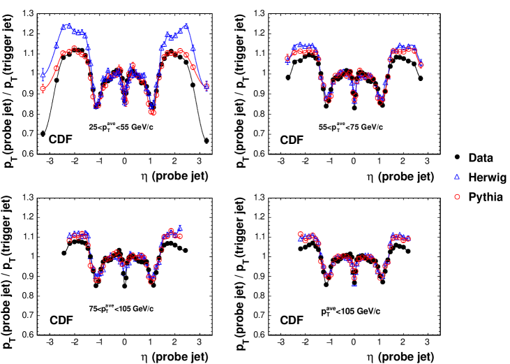
  Abbildung 12: The CDF experiment uses dijet events with a trigger jet within $0.2<|\eta|<0.6$ to obtain $\eta$ dependent corrections to the jet energies. Shown is the ratio of the second (probe) jet $p_{T}$ and the trigger jet $p_{T}$ as a function of probe jet pseudorapidity for various average jet $p_{T}$ regions and for data and Herwig and Pythia simulated events as explained in the figure [63].

  

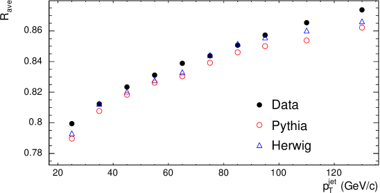
  Abbildung 13: The response for jets in the CDF experiment as a function of the jet transverse momentum, for data as well as simulated events. The response is determined indirectly from the track momenta, and the deviation of the jet response values from $1.0$ is due to the calorimeter response to hadrons being smaller than unity [63].

• Showering Correction $S$: The first two corrections are specific to each experiment and yield jet energies that are independent of the experimental setup, but still depend on the jet finding algorithm. In general, not all energy deposits belonging to the jet are assigned to it by the jet algorithm, and thus a fraction of the energy is not accounted for in the measured jet energy. The energy fraction assigned to the jet is a function of the jet algorithm and its parameters, the jet energy itself, and the pseudorapidity.

The particle jet energy $E^{\rm corr}$ is thus obtained from the raw measured energy $E^{\rm meas}$ as

$$E^{\rm corr}=\frac{E^{\rm meas}(a)-E_{O}\left(a,{\cal L},\eta\right)}{R\left(a,E^{\rm meas},\eta\right)\ S\left(a,E^{\rm meas},\eta\right)}\ ,$$ (9)

where $E_{O}$, $R$, and $S$ are the three corrections described above, depending on the jet algorithm and its parameters, denoted by $a$, the instantaneous luminosity ${\cal L}$, the pseudorapidity $\eta$, and the jet energy itself. An example of the different contributions to the uncertainty on the jet energy scale is given in Figure 14 for the CDF experiment.

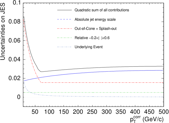
Abbildung 14: The different contributions to the jet energy scale uncertainty at the CDF experiment as a function of the corrected jet $p_{T}$ [63].

This uncertainty on the overall energy scale for jets leads to the dominant systematic error on the top quark mass unless the scale is determined simultaneously with the top quark mass from the same events.

Hadronic $W$ decays in $t\bar{t}$ events provide a means of calibrating the energy scale for light-quark jets with the same event sample for which the calibration is needed to measure the top quark mass. Such an in situ calibration is very attractive experimentally since one becomes independent of uncertainties due to e.g. the photon selection, the jet flavor composition of $\gamma$+jet events, or Monte Carlo simulation. However, at the Tevatron the size of the $t\bar{t}$ event samples is not sufficient to calibrate the jet energy scale as a function of pseudorapidity and energy. Therefore, all jet energy corrections described above are still applied, and in situ calibration is then used only to determine the overall energy scale for all jets. With this approach, the largest part of the jet energy scale systematic error on the top quark mass can still be absorbed in an increased statistical uncertainty. If desired, the information on the overall scale parameter from $\gamma$+jet events or Monte Carlo calibration can be used as an external prior to further reduce the uncertainty. Analyses using in situ calibration are presented in detail in Sections 7.1, 8, and 9.

5.2.2 Bottom-Quark Jet Energy Scale

Even for a given momentum of the parton initiating a jet, both the frequency with which the various hadron species are produced and their momentum spectra are different for quark jets of different flavor or gluon jets. The experiments in general distinguish between bottom-quark and light-flavor jets, where the latter includes any jet that is not initiated by a bottom quark.

Because the particle momentum spectrum differs, the ratio of electromagnetic to hadronic energy is different, thus leading to a different response for bottom-quark and light-flavor jets. A further correction is necessary for jets containing neutrinos which are not measured at all, and for muons which only deposit a small fraction of their energy in the calorimeter. This correction is relevant for jets containing semileptonic heavy hadron decays. An explicit correction can be applied for jets in which the charged lepton is identified inside the jet (only muons are used at the moment). The response for bottom-quark jets without an identified muon will still be shifted due to unidentified semimuonic and semielectronic heavy hadron decays. The showering correction will in principle be different for bottom- and light-flavor jets as well, due to the mass of the decaying bottom hadron.

In practice, the full jet energy corrections are derived as described above for light-flavor jets (for example, most $\gamma$+jet events will not contain bottom-quark jets). For bottom-quark jets, additional corrections are applied to this jet energy scale, and systematic uncertainties are quoted both for the overall (light-flavor) jet energy scale and for the relative scale for bottom-quark and light-flavor jets; for details, see for example [38, 39].

5.2.3 Jet Energy Scale Corrections Specific to $t\bar{t}$ Events

In addition to the general corrections described so far, the CDF experiment applies specific corrections to the energy scale of jets in $t\bar{t}$ events. These corrections account for the $p_{T}$ spectra and jet flavors encountered in $t\bar{t}$ events, which are different from those of the events for which the general corrections have been derived (the jets in $t\bar{t}$ events are initiated by quarks, two of which are bottom quarks, and one charm-quark jet is expected in every second hadronic $W$ decay, while gluon jets are only expected if additional radiation occurs). The corrections are derived from simulated events as described in [38]. Light- and bottom-quark jets are corrected differently, and thus this last correction can only be applied once a jet is assigned to a final parton. In contrast, the D0 experiment absorbs these corrections into the transfer functions used in the Matrix Element and Ideogram analyses. For corrections that are identical for both data and simulation, the measured top quark mass is not systematically shifted since the measurement calibration is based on the simulation. The correction may however lead to an improvement of the statistical sensitivity in template-based measurements where no $m_{t}$ dependent likelihood is derived on an event-by-event basis.

5.2.4 Relative Jet Energy Scale Between Data and Simulation

In all top quark mass measurements, simulated events are used to calibrate the measurement technique. Thus, if the corrected jet energies in the data systematically do not reproduce the particle jet energies, and the same effect is present in Monte Carlo simulated events, the calibration procedure assures that the top quark mass is still measured correctly. Consequently, only uncertainties on the relative data/Monte Carlo jet energy scale enter the systematic error on the top quark mass.

5.2.5 Jet Energy Resolution

For a given event sample and analysis technique the statistical uncertainty on the top quark mass is dominated by the jet energy resolution. To illustrate this, events with a top quark involving a leptonically decaying $W$ have been passed through the full simulation of the D0 detector, and the effect of the detector resolution on the reconstructed top quark mass distribution is studied. Of the three top quark decay products, either for the bottom quark or the charged lepton the reconstructed momentum vector is taken, while the true momentum vectors are used for the other two decay products. The results in the left plot of Figure 15 show that the inclusion of the jet resolution has the largest effect on the distribution of the reconstructed top quark mass. The tails visible when using the reconstructed muon momentum are due to the fact that the momentum resolution degrades with increasing $p_{T}$; the effect on the reconstructed top quark mass distribution is demonstrated in the right plot of Figure 15.

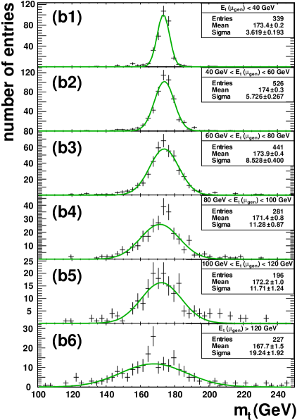
Abbildung 15: Simulated top quark mass distributions for top quark decays at $m_{t}=175\,\,\mathrm{Ge\kern-1.00006ptV}$ involving a leptonic $W$ decay, taking the momentum as reconstructed with the D0 detector for (a) the electron, (b) the muon, or (c) the $b$ jet, and the true momenta for the other two decay products. The effect for muons of different true transverse momentum is shown separately in plots (b1) to (b6). The mean and width of the top quark mass distribution are determined with a Gaussian fit and given in units of GeV.

The CDF experiment has tuned the simulation so that not only the mean shower energy in single track data is reproduced (which is relevant for the overall jet energy scale, see Section 5.2.1), but also the parameters describing the shower shape [63]. Consequently, the jet energy resolution is taken from the simulation.

At the D0 experiment, the jet energy resolution is measured from $\gamma$+jet (below a jet $E_{T}$ of 50 GeV) and dijet events (above 50 GeV). The same measurement is performed in data and Monte Carlo, and the resolution of simulated jets is smeared to reproduce the data. The measured top quark mass depends on the modeling of the jet resolution because the event selection in general requires a minimum jet $E_{T}$. Furthermore, an accurate modeling of the resolution allows the observed statistical error to be compared with expectations from the simulation.

5.3 Efficiency of Bottom-Quark Jet Identification

When the efficiency to identify $b$-quark jets is defined for taggable jets (cf. the definition of taggability in Section 4.3.5), it becomes independent from detector inefficiencies. The taggability is related to the efficiency with which tracks are reconstructed. To take into account the geometrical acceptance of the silicon detector, the D0 experiment measures the taggability of jets in bins of the quantity $\left|z^{\rm pv}\right|\times{\rm sign}\left(z^{\rm pv}\eta^{\rm jet}\right)$ where $z^{\rm pv}$ and $\eta^{\rm jet}$ are the $z$ position of the primary vertex and the pseudorapidity of the jet, respectively [44]. The measured taggability is parametrized as a function of jet transverse momentum and pseudorapidity, and the relative taggabilities of light, charm, and bottom jets are determined from the simulation. The results of the study are shown in Figure 16.

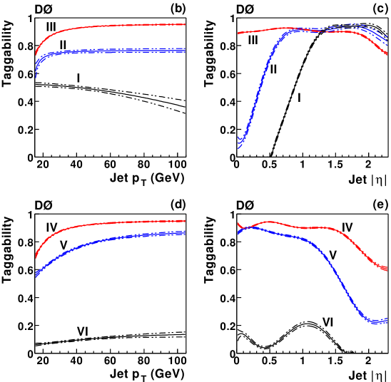
Abbildung 16: Jet taggability measurements by the D0 experiment [44]. (a): Definition of taggability regions. (b)-(e): Taggability measured in the data as a function of jet $p_{T}$ ((b), (d)) and jet $|\eta|$ ((c), (e)) for jets in the various regions defined in (a). (f), (g): Taggability ratios of $b$ to light (full circles) and $c$ to light (open squares) jets determined from simulated events.

Both CDF and D0 determine the $b$-tagging efficiency for bottom-quark jets and the mistag rate for light-flavor jets from data, with additional corrections based on the simulation [44, 46]. The efficiency for bottom-quark jets is measured on a dijet event sample whose bottom-quark content is enhanced by requiring the presence of an electron (CDF) or a muon (D0) within one of the jets as an indication of a semileptonic heavy hadron decay.

The CDF experiment determines the bottom-quark content of their calibration sample by reconstructing $D^{0}\to K^{-}\pi^{+}$ decays or muons in the jet containing the electron, both of which are additional signatures for a heavy hadron decay. The D0 experiment uses the transverse momentum spectrum of the muon relative to the axis of its jet to measure the bottom-quark content of the calibration sample.

Both CDF and D0 thus measure the $b$-tagging efficiency for bottom-quark jets with a semileptonic decay. Corrections to obtain the efficiency for inclusive bottom-quark jets are derived from the simulation. The CDF experiment also takes the dependence of the $b$-tagging efficiency on jet energy, pseudorapidity, and track multiplicity from the simulation, while the overall normalization is determined from the data measurement.

Both CDF and D0 measure the light-flavor tagging rate (mistag rate) on the data using the rate of jets that contain a secondary vertex with negative decay length significance $L_{xy}/\sigma(L_{xy})$ (cf. Section 4.3.5). After correction for the contribution of heavy-flavor jets to such tags and the presence of long-lived particles in light-flavor jets, this rate is a measure of the probability that a light-flavor jet gives a secondary vertex tag with positive $L_{xy}/\sigma(L_{xy})$. The $b$-tagging efficiency for charm-quark jets cannot easily be determined from data, and thus the ratio of efficiencies for charm- and bottom-quark jets is taken from the simulation.

The $b$-tagging efficiencies of the CDF and D0 secondary vertex tagging algorithms for taggable jets are shown in Figure 17.

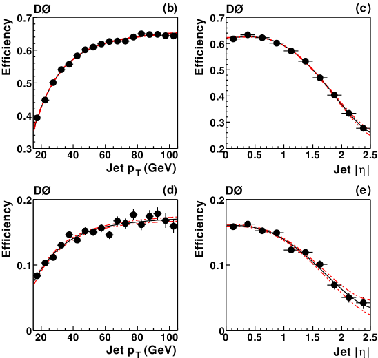
Abbildung 17: Secondary vertex $b$-tagging efficiencies for taggable jets. (a): CDF experiment [38]. Efficiency for bottom-quark jets with $|\eta|<1$ as a function of jet $E_{T}$ together with the $\pm 1\sigma$ uncertainty range. (b)-(e): D0 experiment [44]. Measured efficiency for bottom-quark jets as a function of (b) jet $p_{T}$ and (c) jet $|\eta|$ and for charm-quark jets as a function of (d) jet $p_{T}$ and (e) jet $|\eta|$; the $\pm 1\sigma$ uncertainties of the fits are indicated by the red dotted lines.

6 Methods for Top Quark Mass Measurements

So far, the report described the selection of top-quark events and the calibration of the detectors. This section now introduces a classification of the methods to determine the top quark mass from the events selected. Following this classification, the subsequent sections then give details about each of the methods together with concrete examples.

Experimental results for the top quark mass can be grouped according to the $t\bar{t}$ decay channel analysed, cf. Section 3.2. A comparison between the measurements in different channels allows to search for an indication of differences and thus for new physics effects beyond the Standard Model.

In this section, another classification is introduced according to the measurement technique applied. Even though top quarks decay before hadronization, the information on the top quark mass is still diluted in the events measured in the detector by physics effects (initial- and final-state radiation and hadronization) and the detector resolution. In broad terms, the following different approaches have been followed by the Tevatron experiments to deal with this complication:

Template Method:

A measurement quantity per event called estimator (mostly a single number, but in some measurements a vector of numbers) that is correlated with the top quark mass is computed per event. Any measured quantity in the event that is correlated with the mass of the decaying top quark can be used as estimator in the analysis. In all cases, it is mandatory to understand the exact top quark mass dependence of the distribution of this quantity.

In lepton+jets and all-jets events where enough decay products are reconstructed, the smallest statistical error is obtained if the invariant masses of the two top quarks are explicitly reconstructed to obtain the estimator; this is however not necessary (and not possible in dilepton events without additional assumptions because of the two neutrinos in the final state). In addition, alternative techniques have been developed for lepton+jets events to reduce the sensitivity to systematic errors by a careful selection of the estimator. These are already being explored at the Tevatron and will become much more important at the LHC.

The distribution of the estimator for the set of selected data events is compared with the expected distribution for various assumed values of the top quark mass. This so-called template distribution is generated using simulated signal and background events, taking efficiencies and the relevant cross sections into account. The values of the estimator in the data events are then compared to the template distributions in a fit to determine the top quark mass. To increase the statistical power of the method, the event sample is often divided into subsamples with different signal purity, for example according to the number of $b$-tagged jets per event.

Matrix Element Method:

For each selected event, the likelihood to observe it is calculated as a function of the assumed top quark mass. To this end, all possible reactions yielding final states that could have led to the observed event are considered. An integration is performed over all possible momentum configurations of the final state particles for all relevant reactions. In this integration, the probability of the colliding partons to have a given momentum fraction of the proton or antiproton is taken into account using the appropriate PDFs. Similarly, the likelihood to obtain the detector measurement for an assumed final state is accounted for by a transfer function that relates an assumed final-state momentum configuration to the measured quantities in the detector. Here, a choice can be made which detector measurements to use in the analysis; for example, the measured missing transverse momentum is not explicitly used in the Matrix Element measurements in the lepton+jets channel.

The Matrix Element method accounts for the fact that the accuracy of the information on the top quark mass contained in different events is in general different:

• Depending on the event kinematics and characteristics like the quality of a $b$ tag, some selected events have a higher likelihood of being a $t\bar{t}$ event for a certain top quark mass than others.

• Depending on the energies and directions of the final-state particles, the resolutions of the measured momenta and thus of the top quark mass generally differ between events.

Because a likelihood as a function of assumed top quark mass is calculated separately for each event, and the likelihood for the entire event sample is obtained as the product of the individual event likelihoods, each event contributes to the measurement with its appropriate weight, and the Matrix Element method minimizes the statistical uncertainty of the measurement.

However, the integration over final-state momenta is complex, and it is impossible in practice to use full detector simulation to evaluate the transfer function during the integration. Simplifying assumptions are thus made in the integration, and the measurement is then calibrated using fully simulated events. Still, a Matrix Element measurement requires significantly more computation time than a template analysis. The Matrix Element method was first used by D0 for Tevatron Run I data [65], where it yielded the single most precise measurement, and it also currently yields the single most precise measurement at Run II [66].

Ideogram Method:

The Ideogram method can be regarded as an approximation to the Matrix Element method. It does not make use of the full kinematic characteristics of each selected event, but only relies on information about the invariant masses of the top and antitop quarks and $W$ bosons. The description of wrong jet-parton assignments and of background events is even further simplified.

The statistical sensitivity is not substantially reduced relative to that of the Matrix Element method if the signal to background ratio is large. In particular, the method retains the benefits of using a per-event likelihood as a function of assumed top quark mass. The computations are however simpler than for the Matrix Element method, making the Ideogram method a candidate for future analysis of large-statistics data samples.

If the measured jet energies are used in the computation of the estimator or in the transfer function in order to minimize the statistical uncertainty, the dominant systematic uncertainty is due to the hadronic jet energy scale. The dependence of the top quark mass on external jet energy scale measurements and thus the associated systematic uncertainty is significantly reduced if an overall jet energy scale factor can be fitted simultaneously with the top quark mass using the same $t\bar{t}$ events. The information on the jet energy scale comes mainly from hadronic $W\to q\bar{q}^{\prime}$ decays where a constraint to the known $W$ mass can be used. This in situ calibration also reduces the systematic correlation between measurements on different event samples, which further improves the combination of Tevatron results.

In Section 7 a description of the estimators used in the various template measurements at the Tevatron is given. Section 8 gives details about the computation of the mass-dependent event likelihood in the measurements using the Matrix Element method, and Section 9 outlines the analyses using the Ideogram method. The final top quark mass determination from an event sample is described in Section 10, and systematic uncertainties are discussed in Section 11. Since there is no no a priori fundamental difference between the CDF and D0 experiments on the level of reconstructed $t\bar{t}$ decay products, the following sections describe the measurement techniques based on individual analyses as examples. A full account of all results is given in Section 12.

7 The Template Measurement Method

The template method is the “standard” technique used at the Tevatron to determine the top quark mass from the selected $t\bar{t}$ events. This section introduces the key concept of the template method, the per-event estimator of the top quark mass. Based on recent Tevatron measurements as examples, the calculation of estimators for the various $t\bar{t}$ event topologies is described.

In this section, template-based measurements of the top quark mass are reviewed. The general description of the analyses is complemented with concrete examples from recent Tevatron measurements.

Measurements using the template method are based on the determination of an estimator for each event, which is a quantity that captures the information about the top quark mass contained in the event. Depending on the event topology analyzed, but also depending on the relative importance of statistical and systematic errors, various choices of estimators are possible. In addition, a second estimator is introduced when the jet energy scale is measured simultaneously with the top quark mass. The different choices of estimators used in Tevatron analyses and their computation are described in this section.

The values of the estimator for the selected data events are compared with the expected distribution as a function of the true top quark mass. These expected estimator distributions (templates) are generated using simulated signal and background events for a discrete number of true values of the top quark mass. Trigger and selection efficiencies and the appropriate cross sections (as a function of the top quark mass) are taken into account. The comparison of the sum of signal and background templates for various top quark mass hypotheses with the observed estimator distribution in the data then yields the likelihood to observe this event sample as a function of assumed top quark mass. The top quark mass is usually extracted in a fit of the measured events to the generated template distributions, for which a continuous parametrization of the templates as a function of true top quark mass is obtained. This parametrization is also described in this section. The fitting procedure to determine the top quark mass is then outlined in Section 10.

To the extent that the simulation used to derive the template distributions is accurate, the fit yields a measurement of the true top quark mass. Possible deficiencies of the simulation have to be studied and corresponding systematic uncertainties assigned, as described in general in Section 11.

To extract mass information from the top quark decay products, any measured quantity in the event that is correlated with the mass of the decaying top quark can be used as estimator. In $\ell$$+$jets and all-jets events, taking the explicitly reconstructed invariant top quark mass as estimator allows to extract the largest statistical information per event. An example for the $\ell$$+$jets channel is described in detail in Section 7.1. Alternative estimators have been developed to reduce the sensitivity to systematic uncertainties by a careful selection of the quantity that is used to determine the top quark mass. For an example of a Tevatron study, see Section 7.2. Such techniques will become more important at the LHC with its much larger $t\bar{t}$ data sets. The all-jets decay channel is described in Section 7.3. Dilepton events do not allow a full reconstruction of the event kinematics if the top quark mass is assumed to be unknown. Therefore, techniques have been developed to determine a likely kinematic configuration by making additional assumptions, and the top quark mass reconstructed for this configuration is then used as the estimator, see Section 7.4.

7.1 Full Kinematic Reconstruction of Lepton+Jets Events

The full kinematic reconstruction of $\ell$$+$jets events with a kinematic fit that assumes a $t\bar{t}$ event configuration yields a fitted top quark mass per event that can be used as estimator of the true top quark mass. This technique is most commonly used in template based measurements in the $\ell$$+$jets decay channel at the Tevatron.

The top quark mass information is then mostly based on the measured jets. Both CDF and D0 determine a reference jet energy scale, including $\eta$ and $E_{T}$ dependence, as described in Section 5.2, and correct jet energies and missing transverse momentum according to this scale. With the current Tevatron statistics, measurements in the $\ell$$+$jets channel would be systematically limited by the uncertainty on the overall jet energy scale factor $JES$, unless this factor is determined in situ from the same data as well. The reconstructed hadronic $W$ mass is highly correlated with the jet energy scale, but not with the reconstructed top quark mass. It can therefore be used as an additional estimator to measure an overall deviation from the reference jet energy scale.

As an example, the CDF template measurement [38, 67] is described in detail here.

Event Selection:

The $t\bar{t}$ candidate events are selected by requiring the presence of one electron or muon, missing transverse energy, and four or more jets, as outlined in Section 4.3. The electron (or muon) must have a transverse energy (or momentum) larger than $20\,\,\mathrm{Ge\kern-1.00006ptV}$ and pass quality and isolation criteria, and missing transverse energy of at least $20\,\,\mathrm{Ge\kern-1.00006ptV}$ is required. The transverse energy requirements on the jets (reconstructed with a cone algorithm with radius $\Delta{\cal R}=0.4$ as described in Section 4.3.3) depend on the event category described below.

In hadronic $W$ decays almost exclusively light-quark jets (including charm jets) are produced; thus $b$-tagged jets are likely to be direct top-quark decay products. This analysis does not consider $b$-tagged jets as $W$ decay products. Thus, the number of jet-parton assignments is reduced in events with $b$-tagged jets. As it is then more likely that the kinematic fit selects the correct assignment, the reconstructed mass distribution becomes sharper, and these events contribute more mass information. Furthermore, the signal to background ratio is larger in events with $b$ tags. Finally, the jets in background events have mostly low transverse energies. Consequently, the events are grouped into four categories with different jet $E_{T}$ cuts to improve the statistical error of the measurement. The criteria for the classification are summarized in Table 2.

Category	2-tag	1-tag (T)	1-tag (L)	0-tag
$b$ tagged jets	$n_{b}\geq 2$	$n_{b}=1$	$n_{b}=1$	$n_{b}=0$
$E_{T}$ of three leading jets	$E_{T}\!>\!15\,\,\mathrm{Ge\kern-1.00006ptV}$	$E_{T}\!>\!15\,\,\mathrm{Ge\kern-1.00006ptV}$	$E_{T}\!>\!15\,\,\mathrm{Ge\kern-1.00006ptV}$	$E_{T}\!>\!21\,\,\mathrm{Ge\kern-1.00006ptV}$
$E_{T}$ of fourth jet	$E_{T}\!>\!\enspace 8\,\,\mathrm{Ge\kern-1.00006ptV}$	$E_{T}\!>\!15\,\,\mathrm{Ge\kern-1.00006ptV}$	$E_{T}\!>\!\enspace 8\,\,\mathrm{Ge\kern-1.00006ptV}$	$E_{T}\!>\!21\,\,\mathrm{Ge\kern-1.00006ptV}$
expected $S:B$ ratio	$10.6\,:\,1$	$3.7\,:\,1$	$1.1\,:\,1$	no constraint used

Tabelle 2: CDF lepton+jets template measurement [38]: Event selection requirements for the four categories together with the expected ratios of signal and background events used as constraints in the measurement. Events in the 1-tag (T) category are excluded from the 1-tag (L) category.

Estimator of the Top Quark Mass:

Every selected event is subjected to a kinematic fit, and the jet-parton assignment that yields the best $\chi^{2}$ for a $t\bar{t}$ hypothesis is chosen to compute the estimator of the top quark mass. The fit uses the reconstructed charged lepton, the four highest $E_{T}$ jets, and the unclustered momentum as inputs. Of the 24 possible assignments of four jets to four final-state partons, 12 need not be considered as they correspond to an interchange of the two jets assumed to come from the hadronic $W$ decay, yielding identical reconstructed invariant masses and thus no change to the $\chi^{2}$ value described below. For each of the remaining 12 assignments, two possible solutions for the $z$ component of the neutrino momentum exist for a given value of the $W$ mass. Therefore, 24 different combinations need to be considered in the 0-tag event category; there are 6 combinations for events with one $b$-tagged jet; for 2-tag events, two combinations exist.

The following $\chi^{2}$ is minimized for all different combinations:

$$\chi^{2} = \mathop{\sum_{i=\rm lepton,}}_{\rm 4jets}\frac{\left(p_{T}^{i,\ {\rm fit}}-p_{T}^{i,\ {\rm meas}}\right)^{2}}{\sigma_{i}^{2}}+\sum_{j=x,\,y}\frac{\left({p_{T}^{\rm uncl}}^{j,\ {\rm fit}}-{p_{T}^{\rm uncl}}^{j,\ {\rm meas}}\right)^{2}}{\sigma_{j}^{2}}$$ (10)

$$+\frac{\left(m_{\ell\nu}^{\rm fit}-M_{W}\right)^{2}}{\Gamma_{W}^{2}}+\frac{\left(m_{jj}^{\rm fit}-M_{W}\right)^{2}}{\Gamma_{W}^{2}}+\frac{\left(m_{b\ell\nu}^{\rm fit}-m_{t}^{\rm reco}\right)^{2}}{\Gamma_{t}^{2}}+\frac{\left(m_{bjj}^{\rm fit}-m_{t}^{\rm reco}\right)^{2}}{\Gamma_{t}^{2}}\ .$$

Here, the symbol $p_{T}^{i,\ {\rm meas}}$ denotes the transverse momenta of the charged lepton and four highest $E_{T}$ jets as measured in the detector, and the $\sigma_{i}$ are the corresponding uncertainties. The jet and lepton angles are assumed to be well-measured and are not varied in the fit. The transverse momentum varied in the fit is called $p_{T}^{i,\ {\rm fit}}$. Similarly, the measured unclustered momentum components along $x$ and $y$, their uncertainties, and the fitted unclustered momentum enter the $\chi^{2}$ in the second term. The masses of the two $W$ bosons and the two top quarks in an event need not be equal, but can vary around the $W$ boson mass, $M_{W}=80.42\,\,\mathrm{Ge\kern-1.00006ptV}$, and the reconstructed top quark mass, $m_{t}^{\rm reco}$, according to the decay widths. The Breit-Wigner resonances are approximated with Gaussians with widths $\Gamma_{W}$ and $\Gamma_{t}$. In each step of the minimization procedure the calculated masses $m^{\rm fit}$ are compared with $M_{W}$ and $m_{t}^{\rm reco}$. Note that the quantity $m_{t}^{\rm reco}$ extracted from each event is not a direct measurement of the top quark mass; rather, this quantity is the estimator whose distribution for all data events is then compared with the corresponding distribution in simulated samples. To obtain different values for the two neutrino solutions, the two possible values for the neutrino $z$ momentum are computed assuming the nominal $W$ mass and are used to initialize the fit.

For each event, the estimator $m_{t}^{\rm reco}$ is taken to be the value obtained from the combination that yields the smallest $\chi^{2}$. If this $\chi^{2}$ is greater than 9, the event is rejected altogether from the top quark mass fit. The $m_{t}^{\rm reco}$ distributions for $t\bar{t}$ signal events with $m_{t}=178\,\,\mathrm{Ge\kern-1.00006ptV}$ and the default jet energy scale are shown in Figure 18 for all four event categories. It is evident that events in the 2-tag category have the best $m_{t}^{\rm reco}$ resolution.

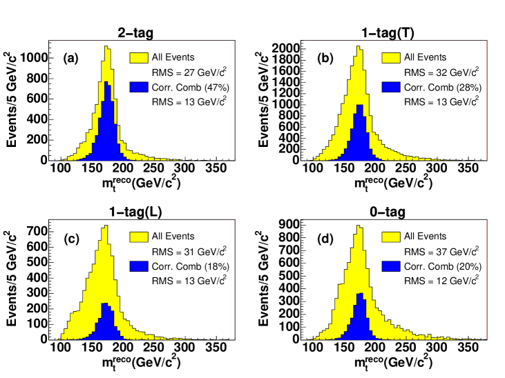
Abbildung 18: CDF lepton+jets template measurement [38]: Template $m_{t}^{\rm reco}$ distributions for simulated signal events with $m_{t}=178\,\,\mathrm{Ge\kern-1.00006ptV}$ and the default jet energy scale in the 2-tag (a), 1-tag(T) (b), 1-tag(L) (c), and 0-tag (d) categories defined in Table 2. The dark blue areas show the distributions for events where the correct jet-parton assignment has been chosen.

Estimator of the Jet Energy Scale:

To determine an estimator of the jet energy scale, no kinematic fit is applied. The masses $m_{jj}$ of all dijet combinations that do not involve a $b$-tagged jet are considered. There are between one (events in the 2-tag category) and 6 (0-tag category) such combinations per event. The $m_{jj}$ distributions for $t\bar{t}$ signal events with $m_{t}=178\,\,\mathrm{Ge\kern-1.00006ptV}$ and the default jet energy scale are shown in Figure 19.

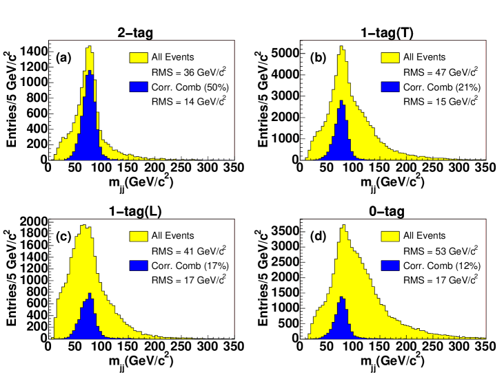
Abbildung 19: CDF lepton+jets template measurement [38]: Template $\mathrm{m}_{jj}$ distributions for simulated signal events with $m_{t}=178\,\,\mathrm{Ge\kern-1.00006ptV}$ and the default jet energy scale in the 2-tag (a), 1-tag(T) (b), 1-tag(L) (c), and 0-tag (d) categories. The dark blue areas show the distributions for dijet pairs that correspond to the $W$ decay products.

Template Parametrization:

The measurements of the top quark mass and the jet energy scale are obtained from an unbinned likelihood fit of the $m_{t}^{\rm reco}$ and $m_{jj}$ values computed in the data events to the predictions from the simulation. However, samples of Monte Carlo simulated events are only available for discrete values of the top quark mass and jet energy scale. The solution is to describe the $m_{t}^{\rm reco}$ and $m_{jj}$ template distributions with functions whose parameters depend on the true values of the top quark mass and jet energy scale. It is then possible to continuously vary the values of the top quark mass and jet energy scale in the fit of the $m_{t}^{\rm reco}$ and $m_{jj}$ values from the data sample. The convention adopted in this measurement is to consider deviations $\Delta_{\rm JES}$ from the reference jet energy scale in units of its uncertainty $\sigma_{c}$ as a function of jet $E_{T}$ and $\eta$, cf. Figure 14.

Examples of Monte Carlo template distributions of $m_{t}^{\rm reco}$ and $m_{jj}$ for signal $t\bar{t}$ events are shown in Figure 20 for various values of the true top quark mass and jet energy scale. The same functional form is used to describe the $m_{t}^{\rm reco}$ and $m_{jj}$ templates. It is a linear combination of two Gaussians with independent parameters (to account for those cases where the $W$ or top quark masses are well-reconstructed, i.e. where the correct combination has been chosen) and a gamma distribution (to describe incorrect combinations). The nine parameters describing a template for a given pair of true ($m_{t}$, $\Delta_{\rm JES}$) values are themselves assumed to depend linearly on both of these true values. This assumption is justified because in the measurement, the values of $m_{t}$ and $\Delta_{\rm JES}$ need only be varied in a relatively small range since they are already known a priori to a certain precision. In Figure 20, the parametrizations of the template distributions are overlaid.

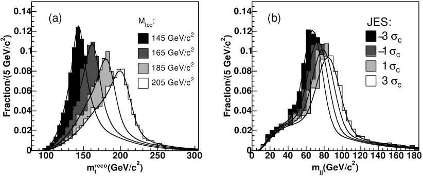
Abbildung 20: CDF lepton+jets template measurement [38]: Template distributions for simulated signal $t\bar{t}$ events in the 1-tag(T) category; (a) $m_{t}^{\rm reco}$ templates for various true top quark masses at $\Delta_{\rm JES}=0$ and (b) $m_{jj}$ templates for various true values of $\Delta_{\rm JES}$ at $m_{t}=180\,\,\mathrm{Ge\kern-1.00006ptV}$. The parametrizations of the template distributions are overlaid.

The $m_{t}^{\rm reco}$ and $m_{jj}$ template distributions for background events do not depend on the true value of the top quark mass. In principle, there is a dependence on the jet energy scale. However, it has been verified that a variation of the jet energy scale affects mostly the overall number of background events while leaving the shape of the template distributions essentially unchanged. The relative contributions of backgrounds from different sources are kept constant, only the overall background normalization is allowed to vary (constrained by the expectation except in the 0-tag category). Therefore, a single $m_{t}^{\rm reco}$ and $m_{jj}$ template distribution is used to describe the background in each event category. The background templates are also described with functions, in this case not to obtain a continuous parametrization but to become insensitive to statistical fluctuations due to the limited size of simulated background samples. As an example, the $m_{t}^{\rm reco}$ and $m_{jj}$ template distributions for background in the 1-tag(T) category are shown in Figure 21 together with their parametrizations.

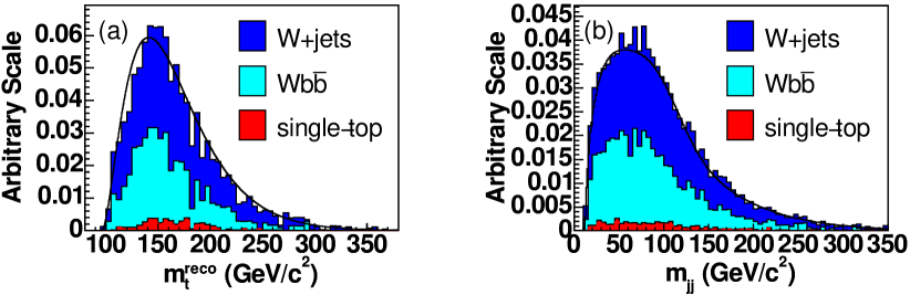
Abbildung 21: CDF lepton+jets template measurement [38]: Template distributions for simulated background events in the 1-tag(T) category with the contributions from individual background sources; (a) $m_{t}^{\rm reco}$ templates and (b) $m_{jj}$ templates. The parametrizations of the template distributions are overlaid.

7.2 Estimators Independent of the Jet Energy Scale

The full kinematic reconstruction of $t\bar{t}$ events in the $\ell$$+$jets channel relies on measurements of four jet energies and thus depends on the determination of the jet energy scale, as explained in the previous section. Measurements that are completely independent of the jet energy scale will be increasingly important for the overall top quark mass combination with decreasing statistical uncertainties. The energy of $b$ quarks from top quark decay is correlated with the top quark mass; the energy of the bottom hadron and consequently its decay length (distance between production and decay vertex) are then also correlated with the top quark mass. The CDF collaboration has used the decay length in the plane perpendicular to the beam axis as an estimator in a top quark mass measurement [68]. This measurement is independent of the jet energy scale (except for the fact that secondary vertices are only looked for in reconstructed jets), but has in principle a larger dependence on modeling of $b$-quark fragmentation than measurements with full reconstruction of the $t\bar{t}$ event kinematics.

The measurement is based on an event sample that is triggered with an inclusive lepton trigger and selected requiring the presence of an isolated charged lepton with $E_{T}>20\,\,\mathrm{Ge\kern-1.00006ptV}$, missing transverse energy $E\kern-6.00006pt/_{T}>20\,\,\mathrm{Ge\kern-1.00006ptV}$, and at least three jets with $E_{T}>15\,\,\mathrm{Ge\kern-1.00006ptV}$, at least one of which is $b$-tagged by the presence of a secondary vertex, as explained in more detail in Section 4.3. Note that it is not necessary to require the presence of four reconstructed jets, as a full reconstruction of the final state is not attempted. The signed decay length $L_{xy}$ corresponding to a secondary vertex is calculated as the vector from the primary to the secondary vertex, projected first onto the jet momentum vector and then into the $xy$ plane perpendicular to the beam axis.

The measurement is based on the mean decay length $\langle L_{xy}\rangle$ in all jets with a secondary vertex with $L_{xy}>0$ in the selected sample. To check the modeling of the decay length, the $L_{xy}$ distributions in doubly $b$-tagged dijet events (which contain mostly $b$-quark jets) and events that contain at most two jets but otherwise pass the $t\bar{t}$ event selection (which are depleted in $b$-quark content) are compared between data and simulation. Decay length values in the simulation are scaled by the ratio between the mean values $\langle L_{xy}\rangle$ found in the data and simulation. In Figure 22, the distribution of positive $L_{xy}$ values measured in the data is shown together with the expected contributions from signal and background events after the scaling procedure.

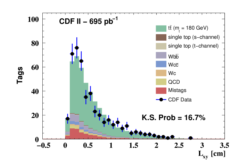
Abbildung 22: CDF lepton+jets measurement using the decay length technique [68]: $L_{xy}$ distribution (from jets with $L_{xy}>0$) in the data (points with error bars) together with the expected contributions from signal and background processes as explained in the plot. The simulated distributions have been normalized to the observed number of events. The result of a Kolmogorov-Smirnov test is indicated in the plot.

The expected distribution of the mean decay length, $\langle L_{xy}\rangle$, is then obtained from pseudo-experiments using simulated events for true values of the top quark mass between 130 and 230  $\mathrm{Ge\kern-1.00006ptV}$. The $\langle L_{xy}\rangle$ values are fitted with a third degree polynomial as a function of $m_{t}$, and this parametrization is used to obtain the measurement of $m_{t}$ from the value of $\langle L_{xy}\rangle$ observed in the data sample.

7.3 Estimators in the All-Jets Channel

As the $\ell$$+$jets channel, the all-jets channel also offers the possibility of full reconstruction of the event kinematics; the challenge here is the large background from QCD multijet events, and also the combinatorial background.

Event Selection:

In the CDF template analysis in the all-jets channel [43, 69], events are used if they pass a multi-jet trigger, contain no isolated energetic leptons and no significant missing transverse energy, and between 6 and 8 jets with $E_{T}>15\,\,\mathrm{Ge\kern-1.00006ptV}$, $|\eta|<2.0$, and $\Delta{\cal R}>0.5$ between the jets. The output of an artificial neural network trained to identify $t\bar{t}$ events is used to further reduce the contribution from QCD multijet background. It is calculated from the following inputs:

• The scalar sum $H_{T}$ of transverse energies of all jets in the event, and the scalar sum of transverse energies of all but the two highest-$E_{T}$ jets;

• the centrality ${\cal C}=H_{T}/\sqrt{\hat{s}}$, where $\sqrt{\hat{s}}$ is the invariant mass of the event calculated from the reconstructed jets, and the aplanarity ${\cal A}=\frac{3}{2}\lambda_{1}$; the symbol $\lambda_{1}$ denotes the smallest of the three eigenvalues of the normalized momentum tensor

  $${\cal M}_{ij}=\frac{\displaystyle\sum_{a}p_{a,i}p_{a,j}}{\displaystyle\sum_{a}\left(\vec{p}_{a}\right)^{2}}\ ,$$ (11)

  where $\vec{p}_{a}$ is the reconstructed momentum vector of jet $a$, and $i$ and $j$ are Cartesian coordinates;

• the minimum and maximum dijet and trijet masses;

• the quantity $E_{T}^{1*}=E_{T}^{1}\sin^{2}\theta_{1}^{*}$, where $E_{T}^{1}$ is the transverse energy of the highest-$E_{T}$ jet in the event, and $\theta_{1}^{*}$ denotes its polar angle in the all-jets rest frame, and the corresponding quantity for the second-highest-$E_{T}$ jet; and

• the geometric average over the $E_{T}^{*}$ values for all but the two highest-$E_{T}$ jets in the event.

The distribution of neural network output values, $NN$, is shown in Figure 23 for the data and the expected $t\bar{t}$ contribution.

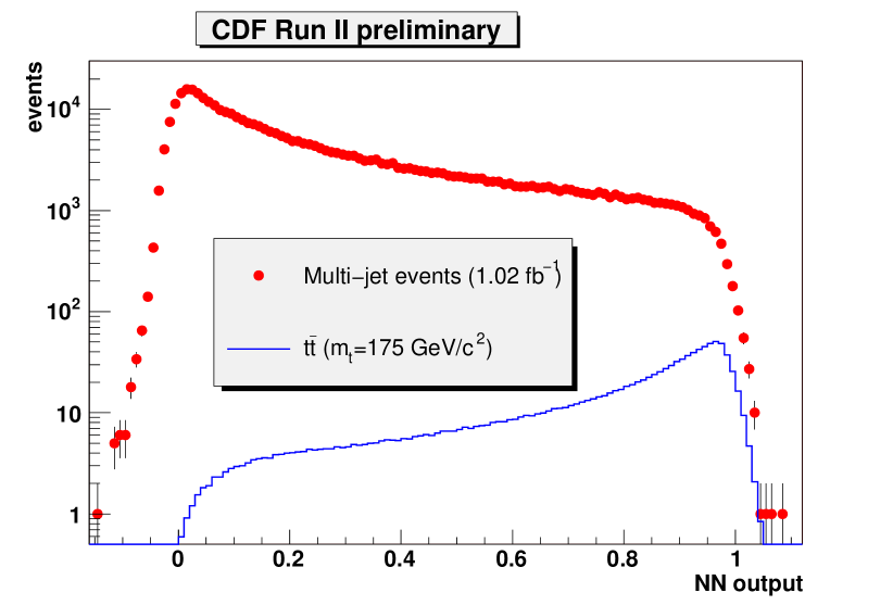
Abbildung 23: CDF all-jets template measurement [69]: Distribution of neural network output values $NN$ for data events (points with error bars) and the expected contribution from $t\bar{t}$ events (solid histogram).

Events are selected if they satisfy $NN>0.91$. The background is further reduced in the subsequent analysis because only events with at least one $b$-tagged jet are used.

Estimator of the Top Quark Mass:

In every selected event, the 6 highest-$E_{T}$ jets are assumed to be $t\bar{t}$ decay products and used to reconstruct the event in a kinematic fit to the $t\bar{t}$ hypothesis similar to the one described in Section 7.1 with a $\chi^{2}$ given by

$$\!\!\!\!\!\!\chi^{2}\!\! \!\!=\!\! \!\!\!\sum_{i=\rm 6\,jets}\frac{\left(p_{T}^{i,\ {\rm fit}}-p_{T}^{i,\ {\rm meas}}\right)^{2}}{\sigma_{i}^{2}}$$ (12)

$$\!\!\!+\frac{\left(m_{\rm dijet\,1}^{\rm fit}-M_{W}\right)^{2}}{\Gamma_{W}^{2}}+\frac{\left(m_{\rm dijet\,2}^{\rm fit}-M_{W}\right)^{2}}{\Gamma_{W}^{2}}+\frac{\left(m_{\rm trijet\,1}^{\rm fit}-m_{t}^{\rm reco}\right)^{2}}{\Gamma_{t}^{2}}+\frac{\left(m_{\rm trijet\,2}^{\rm fit}-m_{t}^{\rm reco}\right)^{2}}{\Gamma_{t}^{2}}\,.\$$

Each $b$-tagged jet is considered in turn as a $b$ jet (with specific $b$-jet energy corrections applied), jet-parton combinations that assign it to a $W$ decay product are rejected, and the reconstructed top quark mass $m_{t}^{\rm reco}$ corresponding to the combination that yields the best $\chi^{2}$ is taken as estimator. Combinations with $\chi^{2}>16$ are rejected. There are thus up to $n_{\rm tag}$ estimators in an event with $n_{\rm tag}$ tagged jets.

Template Parametrization:

Similar to the procedure described in Section 7.1, the $m_{t}^{\rm reco}$ template distributions for various input top quark masses are fitted with functions whose parameters depend on the true value of the top quark mass. Examples of Monte Carlo template $m_{t}^{\rm reco}$ distributions for signal $t\bar{t}$ events are shown in Figure 24(a) for various values of the true top quark mass. The same functional form as in Section 7.1 is used to describe the templates, with linear dependence of the parameters on the true top quark mass.

The background template is derived from the data. The jet tagging probability is obtained from a signal-depleted sample of events with exactly four jets. The background shape is then determined from the $t\bar{t}$ candidate event sample by weighting each jet in turn by its tagging probability, rather than imposing an actual $b$-tagging requirement. The signal contribution to this background template estimate is obtained using the simulation and subtracted. The procedure for determining the background shape is validated using events with low neural network output $NN$. The background template, shown in Figure 24(b), is parametrized with two gamma functions plus one Gaussian.

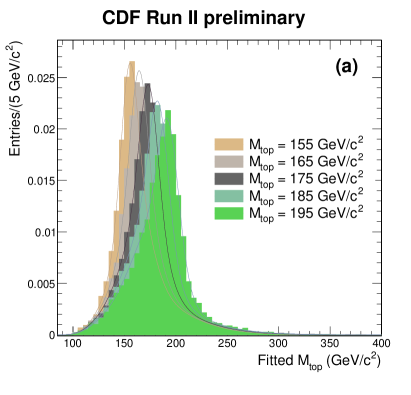
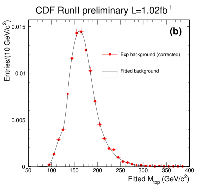
Abbildung 24: CDF all-jets template measurement [69]: Template $m_{t}^{\rm reco}$ distributions for (a) signal $t\bar{t}$ events for various true top quark masses and (b) background events. The parametrizations of the template distributions are overlaid.

7.4 Estimators in the Dilepton Channel

As explained in Section • ‣ 3.2, dilepton events are kinematically underconstrained if the top quark mass is not assumed to be known. It is therefore not possible to use full reconstruction of the event kinematics to obtain an estimator $m_{t}^{\rm reco}$ as in the $\ell$$+$jets or all-jets channels, cf. Sections 7.1 and 7.3. Nevertheless, for a given selected dilepton event, some top quark mass hypotheses are still more likely than others, and this allows a top quark mass measurement. To determine the relative likelihoods of different top quark mass assumptions, an integration is performed over undetermined kinematic quantities of the event. Various methods have been developed for this integration and for obtaining a top quark mass estimator; in the following, these methods are described in turn. The event selection criteria for all analyses are based on the general topology of a dilepton $t\bar{t}$ event as described in Section 4.4.1: Typically, two oppositely-charged isolated energetic leptons inconsistent with the $Z\to\ell^{+}\ell^{-}$ hypothesis, at least two energetic jets, and significant missing transverse energy are required, and the two highest-$E_{T}$ jets are assumed to be $t\bar{t}$ decay products.

Neutrino Weighting Method:

This method has been used by both CDF and D0 in Run I [70] and Run II [71, 72]. Since the $b$ and $\overline{b}$ jets are not distinguished in the reconstruction, there are two possible jet-parton assignments, corresponding to two possible jet-lepton pairings per event. For each pairing, a scan over assumptions for $m_{t}$ and the (anti-)neutrino pseudorapidities $\eta_{\nu}$ and $\eta_{\overline{\nu}}$ is performed. Disregarding the measured missing momentum in the event, the event kinematics are reconstructed for each assumption by imposing a $t\bar{t}$ event hypothesis. This leads to four solutions per $\left(m_{t},\ \eta_{\nu},\ \eta_{\overline{\nu}}\right)$ assumption. According to the measured missing transverse momentum $\vec{p}\kern-4.49997pt/_{T}$, each solution $i$ is assigned a weight $w_{i}$ of

$$w_{i}=\exp\left(-\frac{\left(p\kern-4.49997pt/_{x}-p_{\nu,x}-p_{\overline{\nu},x}\right)^{2}}{2\sigma_{x}^{2}}\right)\exp\left(-\frac{\left(p\kern-4.49997pt/_{y}-p_{\nu,y}-p_{\overline{\nu},y}\right)^{2}}{2\sigma_{y}^{2}}\right)\ ,$$ (13)

where $\left(\sigma_{x},\ \sigma_{y}\right)$ denotes the missing transverse momentum resolution, and $\vec{p}_{\nu}$ and $\vec{p}_{\overline{\nu}}$ are the neutrino momenta obtained for the given solution. For a given assumption, the four solutions have equal a priori probability; the assumption can thus be assigned a weight of

$$w\left(m_{t},\ \eta_{\nu},\ \eta_{\overline{\nu}},\ {\rm pairing}\right)=\sum_{i=1}^{4}w_{i}\ .$$ (14)

The a priori probabilities of the neutrino and antineutrino pseudorapidities are determined from simulated $t\bar{t}$ events. They are uncorrelated and can be described by a Gaussian centered around zero whose width is nearly independent of the true top quark mass (cf. Figure 25). To obtain the weight as a function of the top quark mass alone, a scan over the unknown values of $\eta_{\nu}$ and $\eta_{\overline{\nu}}$ is performed, and the corresponding weights are multiplied with the a priori probabilities $P\left(\eta_{\nu},\ \eta_{\overline{\nu}}\right)$ of the neutrino and antineutrino pseudorapidities. Finally, as both jet-lepton pairings also have the same a priori probability, one obtains

$$w(m_{t})=\sum_{\rm pairings\ }\sum_{\,\eta_{\nu},\,\eta_{\overline{\nu}}}P\left(\eta_{\nu},\ \eta_{\overline{\nu}}\right)w\left(m_{t},\ \eta_{\nu},\ \eta_{\overline{\nu}},\ {\rm pairing}\right)\ .$$ (15)

While the weight distribution $w(m_{t})$ for a single event can have more than one relative maximum, the average weight distribution for many simulated events has one maximum close to the true top quark mass, as shown in Figure 26.

Abbildung 25: CDF dilepton neutrino weighting template measurement [71]: The distribution of neutrino pseudorapidities $\eta$ with a Gaussian fit (upper left) and the correlation with the antineutrino pseudorapidity (upper right), determined from simulated $t\bar{t}$ events with $m_{t}=178\,\,\mathrm{Ge\kern-1.00006ptV}$ using herwig Monte Carlo. The width of the fitted Gaussian as a function of $m_{t}$ is shown in the lower plot; here, the line indicates the width for $m_{t}=178\,\,\mathrm{Ge\kern-1.00006ptV}$.

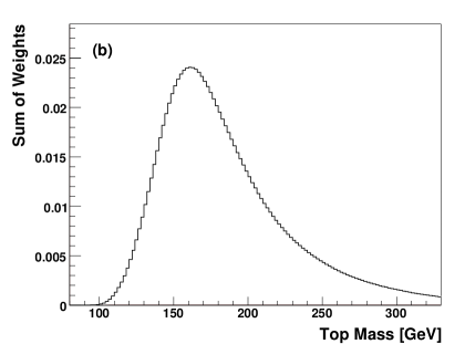
Abbildung 26: Dilepton neutrino weighting template measurements: (a) The weight distribution as a function of assumed top quark mass for one $t\bar{t}$ event with $m_{t}=170\,\,\mathrm{Ge\kern-1.00006ptV}$ simulated using herwig, reconstructed at CDF [71]. The top quark mass value taken as estimator for this event is indicated by the vertical line. (b) The average weight distribution (obtained by summing weights for many simulated events) for $t\bar{t}$ events with $m_{t}=175\,\,\mathrm{Ge\kern-1.00006ptV}$ generated with pythia, reconstructed at D0 [72].

Both CDF [71] and D0 [72] have performed measurements where the $m_{t}$ value that maximizes the weight distribution is taken as the top quark mass estimator for a given event. These analyses then proceed as described above in Section 7.1: The templates are fitted as a function of the most likely top quark mass, and for the signal templates, the dependence of the fit parameters on the true top quark mass is parametrized as well [71] or included in a two-dimensional fit of the templates as a function of the estimator value and the true input top quark mass [72].

This procedure where the $m_{t}$ value that maximizes the weight is taken as estimator does not take into account that events with a broad maximum contain less $m_{t}$ information than events where the maximum is strongly peaked. D0 has therefore made measurements that use a vector of estimators. This vector either contains the weight histogram integrated in a few coarse bins or the mean and RMS of the weight distribution [72]. These multidimensional estimators cannot be fitted like in the one-dimensional case; therefore, the signal and background probability densities for a given vector of estimators are determined from the density and weights of simulated events with estimators that have nearby values in estimator-space. A parametrization of probability densities as a continuous function of assumed top quark mass is not performed, either. The gain from these methods is modest: D0 finds that relative to the analysis that uses as estimator the $m_{t}$ value that maximizes the weight, the expected uncertainty decreases by 7% when using five bins, but even increases by 5% when using the mean and RMS [72]. Rather than introducing multidimensional estimators for the same quantity, a more natural approach to extracting more information from the events is to go beyond template methods altogether, as described for example in Section 8.

Neutrino $\phi$ Weighting Method:

Instead of assuming the pseudorapidities $\eta$ for both neutrino momenta, one can assume values of their azimuthal angles. This procedure is used by CDF [71]. A top quark mass estimator for a selected event is obtained via the following steps:

• For each assumed pair of neutrino $\phi$ values, the event kinematics is reconstructed in a kinematic fit assuming a $t\bar{t}$ event that constrains the lepton-neutrino pairs to the $W$ boson mass and constrains the two top quarks to have equal masses within the top quark width. For each pair, there are 8 solutions arising from the two-fold ambiguity in solving for the neutrino longitudinal momentum and from the two lepton-jet pairings, and the fitted top quark mass from the solution with the smallest $\chi^{2}$ is taken.

• A $12\times 12$ grid of assumed neutrino $\phi$ values is tested. The top quark mass calculated for each given pair of assumed neutrino $\phi$ values is weighted by its $\chi^{2}$ probability. The weighted average of the top quark masses is then taken as estimator for the event, where only assumptions with a weight of at least 30% of the maximum weight in the event are considered.

Full Kinematic Analysis:

A third method employed by CDF uses an assumed value $p_{z}(t\bar{t})$ of the longitudinal momentum component of the $t\bar{t}$ system to solve the event kinematics [71]. The $p_{z}(t\bar{t})$ distribution is expected to be centered around zero with a width of $180\,\,\mathrm{Ge\kern-1.00006ptV}$, where the width changes by $10\%$ when varying the top quark mass between $140$ and $200\,\,\mathrm{Ge\kern-1.00006ptV}$. There are two possible jet-lepton pairings, each with up to four different solutions to the kinematic equations for a given assumed value of $p_{z}(t\bar{t})$. The up to eight possible solutions for the top quark mass under the assumption of a $t\bar{t}$ event are calculated. This procedure is repeated 10000 times, with $p_{z}(t\bar{t})$ values drawn from the expected distribution, and with the measured jet energies and the missing momentum varied within their resolutions. Of the four most probable values corresponding to the four solutions for a given jet-lepton pairing, the one yielding the smallest $t\bar{t}$ invariant mass is retained, if any solution was found.

From the resulting distributions of top quark masses for each of the two jet-lepton pairings, the one pairing is chosen for which the number of trials that yielded no solution is smaller. The most probable value of the corresponding distribution of top quark mass solutions is taken as the estimator. The procedure slightly favors lower top quark masses; however this is valid since only an estimator for the top quark mass is desired, and the bias introduced is corrected for when the method is calibrated using simulated events.

Matrix Weighting Method:

In the Matrix Weighting technique employed by D0 [73] the kinematics of the $t\bar{t}$ candidate event is solved by assuming a value for the top and antitop quark masses. There are four solutions to the kinematic equations for a given jet-lepton pairing. The weight for a given solution is computed from the proton and antiproton parton distribution functions $f_{\rm PDF}$ and $\bar{f}_{\rm PDF}$ and the probability $p\left(E_{\ell}^{*}|m_{t}\right)$ of a charged lepton $\ell$ to have energy $E_{\ell}^{*}$ in the top quark rest frame as

$$w=f_{\rm PDF}(x)\bar{f}_{\rm PDF}(\overline{x})p\left(E_{\ell}^{*}|m_{t}\right)p\left(E_{\overline{\ell}}^{*}|m_{t}\right)\,,$$ (16)

where $x$ and $\overline{x}$ denote the momentum fractions of the colliding partons in the proton and antiproton. To compute the total weight for a given $m_{t}$ assumption, the weights for both jet-parton assignments and all solutions are summed. Using resolution sampling, the above procedure is repeated many times with reconstructed energies/momenta and the missing transverse momentum drawn from distributions according to the detector resolution, and for each assumed top quark mass, the mean total weight is determined. The value of the assumed top quark mass where the mean total weight reaches its maximum is then taken as the estimator for the measurement.

8 The Matrix Element Measurement Method

The previous section described different possibilities for computing an estimator of the top quark mass in each $t\bar{t}$ candidate event, and how the expected estimator distribution as a function of the assumed top quark mass can be used in a top quark mass measurement. In this section, a different measurement strategy is described, where for each selected event a likelihood as a function of the assumed top quark mass is calculated. The section starts with the definition of this likelihood, then describes the parametrization of the detector resolution needed to compute it, and continues with an in-depth discussion of how the likelihood is calculated for the various (signal and background) processes via which a candidate event may have been produced.

The Matrix Element method is based on the likelihood to observe a given event in the detector, calculated as a function of assumed top quark mass. The Matrix Element method was first used by the D0 collaboration for the measurement in the $\ell$$+$jets channel at Tevatron Run I [65], where it yielded the single most precise measurement of the top quark mass. The method has been applied to the measurement in the $\ell$$+$jets channel at Run II by both CDF [66] and D0 [39], and CDF has also used it in the dilepton channel [74, 75, 76]. The Dynamical Likelihood method follows a similar concept. It has been used by CDF in the $\ell$$+$jets [57] and dilepton [77] channels at Run II and is described in this section together with the Matrix Element method.

The selection of events used in the analyses is briefly described in Section 8.1. An overview of the calculation of the event likelihood is given in Section 8.2, and the calculation of the likelihood for a given process is explained in Section 8.3. Section 8.4 discusses the parametrization of the detector response. This includes a description of how $b$-tagging information can be used in the analysis. Technical details on the computation of the signal and background likelihoods are given in Sections 8.5 and 8.6 with an emphasis on the D0 Run II analysis in the $\ell$$+$jets channel which serves as an example.

8.1 Event Selection

The selection of events for the measurements with the Matrix Element method is very similar to the general criteria described in Sections 4.4.1 and 4.4.2 and to the selections used in measurements based on the template method, see Section 7.

There is, however, one aspect that deserves special attention. Leading-order matrix element calculations are used to evaluate likelihoods with which the selected events are produced in the signal and background processes. Initial- and final-state gluon radiation are therefore not accounted for in these likelihoods. This is not a problem since the calibration of the measurement is based on fully simulated events which do include gluon radiation, cf. Section 10.2. Nevertheless, both CDF and D0 select only events with exactly four jets for their Matrix Element measurements in the $\ell$$+$jets channel. While not completely removing events with significant gluon radiation, this cut still reduces their contribution to the event sample. Also, the complication of selecting the jet from radiation and assigning it either to initial-state radiation or to final-state radiation off one of the $t\bar{t}$ decay products is avoided. On the other hand, the measurements in the dilepton channel are more severely limited by statistics. Here the event selection requires two or more jets, as for the template analyses, and any jets but the two highest-$E_{T}$ ones are assumed to be due to initial-state radiation.

In the $\ell$$+$jets channel, the D0 experiment has performed both a topological and a $b$-tagging measurement (i.e. disregarding/using $b$-tagging information); in both analyses, all events (irrespective of the number of $b$ tags) are used. Unless noted explicitly, the following description refers to the $b$-tagging analysis. In contrast, the CDF event selection in the $\ell$$+$jets channel requires at least one jet to be $b$-tagged; this selection is used in the Matrix Element and also the Dynamical Likelihood measurement. In the dilepton channel, CDF has performed two measurements based on the Matrix Element method, one not using $b$-tagging information and the other requiring at least one $b$-tagged jet. The dilepton measurement with the Dynamical Likelihood technique does not use $b$-tagging information.

8.2 The Event Likelihood

To make maximal use of the kinematic information on the top quark mass contained in the event sample, for each selected event the likelihood $L_{\rm evt}$ that this event is observed is calculated as a function of the assumed top quark mass. In analyses where additional parameters like the overall jet energy scale are to be measured simultaneously with the top quark mass, $L_{\rm evt}$ is also a function of the assumed values of these parameters. The likelihoods for all events are then combined to obtain the sample likelihood, and the measurement of the top quark mass and of the other parameters, if applicable, is extracted from this sample likelihood. To make the likelihood calculation tractable, simplifying assumptions in the description of the physics processes and the detector response are introduced as described in this section. Before applying it to the data, the measurement technique is however calibrated using fully simulated events, and the assumptions the full simulation makes to describe the physics processes are accounted for by systematic uncertainties.

It is assumed that the physics processes that can lead to an observed event do not interfere. The likelihood $L_{\rm evt}$ then in principle has to be composed from likelihoods for all these processes as

$$L_{\rm evt}=\sum_{{\rm processes}\ P}f_{P}L_{P}\ ,$$ (17)

where $L_{P}$ is the likelihood for the event to be created via a given process $P$, and $f_{P}$ denotes the fraction of events from that process in the event sample. In practice, not all possible processes can be accounted for explicitly, and simplifying assumptions are made in the calculation of the likelihoods for the individual processes. The measurement result therefore has to be corrected accordingly.

A likelihood $L_{t\bar{t}}$ is calculated for the event to be produced in the signal $t\bar{t}$ reaction; this likelihood will depend on the assumed top quark mass. The $t\bar{t}$ production processes taken into account are listed in Table 3. In their measurements using the Matrix Element method, CDF and D0 have also included likelihoods for the event to be produced via the dominant background processes; this maximizes the separation between signal and background events and keeps corrections to the final result small. In contrast, the CDF analyses using the Dynamical Likelihood technique omit an explicit treatment of background at this stage and apply a correction for all backgrounds to the final result. When applying the Matrix Element method to the $\ell$$+$jets channel, CDF and D0 choose to determine the jet energy scale and the signal fraction together with the top quark mass.

The event likelihood $L_{\rm evt}$ can thus be expressed as

$$L_{\rm evt}\left(x;\,m_{t},JES,f_{t\bar{t}}\right)=f_{t\bar{t}}L_{t\bar{t}}\left(x;\,m_{t},JES\right)+\left(1-f_{t\bar{t}}\right)L_{\rm bkg}\left(x;\,JES\right)\ ,$$ (18)

where $L_{\rm bkg}$ is a weighted sum of likelihoods for all background processes according to Equation (17). The symbol $x$ denotes the kinematic variables of the event, $f_{t\bar{t}}$ is the signal fraction of the event sample, and $L_{t\bar{t}}$ and $L_{\rm bkg}$ are the likelihoods for observing the event if it is produced via the $t\bar{t}$ or any of the background processes, respectively. The values of $f_{t\bar{t}}$ and $JES$ are fixed if applicable, depending on the details of the analysis. An overview of the event likelihood calculation in the analyses described here is given in Table 3.

channel	method	exp.	parameters	signal processes	background processes	reference
$\ell$$+$jets	ME	D0	$m_{t}$, $JES$, $f_{t\bar{t}}$	$q\bar{q}\to t\bar{t}$	$W\!+\!{\rm\text{4}p}$	[39]
$\ell$$+$jets	ME	CDF	$m_{t}$, $JES$, $f_{t\bar{t}}$	$q\bar{q}\to t\bar{t}$	$W\!+\!{\rm\text{4}p}$	[66]
$\ell$$+$jets	DL	CDF	$m_{t}$	$q\bar{q}\to t\bar{t}$, $gg\to t\bar{t}$	—	[57]
dilepton	ME	CDF	$m_{t}$	$q\bar{q}\to t\bar{t}$	$Z/\gamma^{*}$$+$2p, $WW$$+$2p, $W$$+$3p	[74, 75]
dilepton	DL	CDF	$m_{t}$	$q\bar{q}\to t\bar{t}$, $gg\to t\bar{t}$	—	[77]

Tabelle 3: Overview of the $L_{\rm evt}$ calculation in the $m_{t}$ measurements using the Matrix Element (ME) and Dynamical Likelihood (DL) methods. The column entitled “parameters” lists the quantities that are measured in the analysis, and the signal and background processes taken into account in the event likelihood are listed in the following columns. The symbol “p” refers to any light parton, i.e. a $u$, $d$, $s$, or $c$ quark (or antiquark) or a gluon. The lines describing the Matrix Element measurements by D0 in the $\ell$$+$jets channel and by CDF in the dilepton channel refer to both the topological and the $b$-tagging analyses (the $WW$$+$2p background is negligible and not considered in the dilepton measurement using $b$ tagging).

To extract the top quark mass from a set of $N$ measured events $x_{1},..,x_{N}$, a likelihood function for the event sample is built from the individual event likelihoods calculated according to Equation (18) as

$$L(x_{1},..,x_{N};\,m_{t},JES,f_{t\bar{t}})=\prod_{i=1}^{N}L_{\rm evt}(x_{i};\,m_{t},JES,f_{t\bar{t}})\,.$$ (19)

This likelihood is maximized to determine the top quark mass (and additional parameters, if applicable).

8.3 The Likelihood for one Process

To evaluate the likelihood for an observed event to be produced via a given process $P$, all possible configurations $y$ of the four-momenta of the final-state particles that could have led to the observed event $x$ are considered. In practice, also a sum over different non-interfering processes is performed; thus only one likelihood is computed for different color or flavor configurations if the differential cross section is identical. The likelihood for a final state with $n_{f}$ partons and given four-momenta $y$ to be produced in the hard-scattering process is proportional to the differential cross section ${\rm d}\sigma_{P}$ of the corresponding process, given by

$${\rm d}\sigma_{\!P}(a_{1}a_{2}\to y)=\frac{(2\pi)^{4}\!\left|\mathscr{M}_{P}\left(a_{1}a_{2}\to y\right)\right|^{2}}{\xi_{1}\xi_{2}s}{\rm d}\Phi_{n_{f}}\ ,$$ (20)

where $a_{1}a_{2}$ and $y$ stand for the kinematic variables of the partonic initial and final state, respectively. The symbol $\mathscr{M}_{P}$ denotes the matrix element for this process, $s$ is the center-of-mass energy squared of the collider, $\xi_{1}$ and $\xi_{2}$ are the momentum fractions of the colliding partons $a_{1}$ and $a_{2}$ (which are assumed to be massless) within the colliding proton and antiproton, and ${\rm d}\Phi_{n_{f}}$ is an element of $n_{f}$-body phase space.

To obtain the differential cross section ${\rm d}\sigma_{\!P}(p\bar{p}\to y)$ in $p\bar{p}$ collisions, the differential cross section from equation (20) is convoluted with the parton density functions (PDF) and summed over all possible flavor compositions of the colliding partons,

$${\rm d}\sigma_{\!P}(p\bar{p}\to y)=\int\limits_{\xi_{1},\xi_{2}}\sum_{a_{1},a_{2}}{\rm d}\xi_{1}{\rm d}\xi_{2}\ f_{\rm PDF}^{a_{1}}(\xi_{1})\ \bar{f}_{\rm PDF}^{a_{2}}(\xi_{2})\ {\rm d}\sigma_{\!P}(a_{1}a_{2}\to y)\ ,$$ (21)

where $f_{\rm PDF}^{a}(\xi)$ and $\bar{f}_{\rm PDF}^{a}(\xi)$ denote the probability densities to find a parton of given flavor $a$ and momentum fraction $\xi$ in the proton or antiproton, respectively. This equation directly reflects QCD factorization as introduced in Section 3.1 and corresponds to Equation (5).

The finite detector resolution is taken into account via a convolution with a transfer function $W(x,y;\,JES)$ that describes the probability to reconstruct a partonic final state $y$ as $x$ in the detector. The differential cross section to observe a given reconstructed event then becomes

$${\rm d}\sigma_{\!P}(p\bar{p}\to x) = \int\limits_{y}{\rm d}\sigma_{\!P}(p\bar{p}\to y)\ W(x,y;\,JES)\ .$$ (22)

Only events that are inside the detector acceptance and that pass the trigger conditions and offline event selection are used in the measurement. Because of the selection cuts, the corresponding overall detector efficiency depends both on $m_{t}$ and on the jet energy scale. This is taken into account in the cross section of events observed in the detector:

$$\sigma_{\!P}^{\rm obs}=\int\limits_{x,y}{\rm d}\sigma_{\!P}(p\bar{p}\to y)W(x,y;\,JES)f_{\rm acc}(x){\rm d}x\ ,$$ (23)

where $f_{\rm acc}=1$ for selected events and $f_{\rm acc}=0$ otherwise.

For example, the likelihood to observe a $t\bar{t}$ event as $x$ in the detector is given by

$$L_{t\bar{t}}(x;\,m_{t},JES) = \frac{{\rm d}\sigma_{t\bar{t}}(p\bar{p}\to x;\,m_{t},JES)}{\sigma^{\rm obs}_{t\bar{t}}(m_{t},JES)}$$

$$= \frac{1}{\sigma^{\rm obs}_{t\bar{t}}(m_{t},JES)}\int\limits_{\xi_{1},\xi_{2},y}\sum_{a_{1},\,a_{2}}{\rm d}\xi_{1}{\rm d}\xi_{2}\,f_{\rm PDF}^{a_{1}}(\xi_{1})\,\bar{f}_{\rm PDF}^{a_{2}}(\xi_{2})\,\times$$

$$\frac{(2\pi)^{4}\left|\mathscr{M}_{t\bar{t}}(a_{1}a_{2}\to y)\right|^{2}}{\xi_{1}\xi_{2}s}{\rm d}\Phi_{6}W(x,y;\,JES)\ .$$

The contributions to the likelihood are visualized schematically in Figure 27. A similar formula holds for the likelihood to observe a background event as $x$, except this likelihood does not depend on the top quark mass.

Abbildung 27: Schematic representation of the calculation of the likelihood for $t\bar{t}$ production to lead to a given observed $\ell$$+$jets event. The observed event $x$, shown in red at the right, is fixed while integrating over all possible momentum configurations $y$ of final-state particles (shown in blue). All possible assignments of final-state partons arising from the process shown by the Feynman diagram to the measured jets in the detector are considered (only one possibility is shown here). The differential cross section for the process shown by the diagram is convoluted with the probability for the final-state partons to yield the observed event (transfer function), and with the probability to find initial-state partons, shown in green to the left, of the given flavor and momenta inside the colliding proton and antiproton (parton distribution function). For each partonic final state under consideration, the initial state parton momenta are known by energy and momentum conservation.

Details of the parametrization of the detector response are given in Section 8.4. The parametrization of the matrix element and the computation of $L_{t\bar{t}}$ are described in Section 8.5. The determination of $L_{\rm bkg}$ is discussed in Section 8.6.

8.4 Description of the Detector Response

The transfer function $W(x,y;\,JES)$ relates the characteristics $y$ of the final-state partons to the measurements $x$ in the detector. The symbol $x$ denotes measurements of the jet and charged lepton energies or momenta and directions as well as $b$-tagging information for the jets. A parametrization of the detector resolution is used in the likelihood calculation because the full geant-based simulation would be too slow. The full simulation is however used to generate the simulated events with which the method is calibrated. In this section, the general form of the transfer function is first described, followed by a discussion of the individual factors.

8.4.1 General Form of the Transfer Function

The transfer function $W(x,y;\,JES)$ describes the probability density ${\rm d}P$ to reconstruct a given assumed partonic final state $y$ as $x$ in the detector:

$${\rm d}P=W(x,y;\,JES){\rm d}x\ .$$ (25)

Because the final-state partons are assumed to give rise to some measured event $x$, the normalization condition

$$\int_{x}W(x,y){\rm d}x=1$$ (26)

holds, where the integral is over all possible observed events $x$.

The transfer function is assumed to factorize into contributions from each measured final-state particle. Aspects to be considered in the transfer function are in principle the measurement of the momentum of a particle (both of its energy and of its direction) as well as its identification.

The relative importance of the energy resolution for electrons, muons, and quarks for the top quark mass reconstruction has been studied qualitatively in simulated top quark decays with a leptonic $W$ decay, reconstructed with the D0 detector. Of the three top quark decay products, the reconstructed momentum from either the charged lepton or the $b$ jet is taken, while the true values are taken from the simulation for the other two particles. The three plots in Figures 15(a), (b), and (c) show qualitatively that the resolution of the top quark mass is dominated by the jet energy resolution, while the effect of the electron resolution is comparatively small. The effect of the muon resolution at high muon transverse momentum is of the same order as that of the jet resolution, while muons are comparatively well-measured at low $p_{T}$, as shown in Figures 15(b1)-(b6).

Consequently, the following assumptions are made about how final-state particles are measured in the detector, which allow reducing the dimensionality of the integration over 6-particle phase space described in Section 8.3:

• Electrons: Apart from efficiency losses (which are not described by the transfer function), electrons are assumed to be unambiguously identified (i.e. an electron is not reconstructed as a muon or a hadronic jet). The electron direction and energy are both assumed to be well-measured, i.e. during integration, the final-state electron is assumed to be identical to the measured particle.

• Muons: As for electrons, muons are assumed to be unambiguously identified, and their direction to be precisely measured. While CDF also considers the muon $p_{T}$ to be well-measured, D0 introduces a transfer function that allows for a finite resolution. This has primarly an effect for muons with large $p_{T}$.

• Energetic quarks and gluons: Energetic quarks and gluons are almost always reconstructed as a jet in the detector. There is however a small probability that they are reconstructed as an isolated fake lepton, and it depends on the process considered whether or not this possibility has to be taken into account: If the number of energetic leptons required in the event selection is already present in the final state, the possiblity that this lepton is not reconstructed and a quark/gluon fakes a lepton that is selected can be ignored. If fewer energetic leptons are produced than required in the selection, it is assumed that the signatures of the remaining leptons in the detector have arisen from quarks or gluons. This effect becomes important in the case of dilepton events, where background from $W$$+$3p production is explicitly taken into account.

  Both D0 and CDF assume the direction of the final-state quarks and gluons to be well-measured by the jet directions. Transfer functions are introduced for the jet energy (or transverse energy).

  The ability of the detector to distinguish quarks and gluons and to identify the flavor of final-state quarks is limited. The probability to obtain a $b$-tagged jet is largest for $b$ quarks, and it is still larger for $c$ quarks than for light quarks or gluons. While the D0 measurement takes into account the possibility that a $b$ tag is faked by a $c$ or light quark or gluon, CDF makes the approximation that this probability is zero for signal events where enough $b$ quarks are present in the final state. This has consequences for the assignment of final-state quarks to measured jets in $\ell$$+$jets $t\bar{t}$ events, where there are two $b$ quarks and two light (or charm) quarks in the final state. In dilepton $t\bar{t}$ events with only two $b$ quarks in the final state, this complication does not arise.

• Neutrinos: Neutrinos are not measured in the detector. The presence of energetic neutrinos can be inferred from the transverse momentum imbalance ($\vec{p}\kern-4.49997pt/_{T}$); however this quantity depends on the momenta of the other objects measured in the detector. The observed missing transverse momentum is due to the neutrinos as well as to mismeasurement of jet energies and of the energy $E_{T,{\rm recoil}}$ from other objects in the detector against which the $t\bar{t}$ system recoils.

  In the Matrix Element analyses, the $t\bar{t}$ transverse momentum is assumed to be zero, and the transverse components of the sum of neutrino momenta is obtained as the negative vector sum of all other assumed final-state particle transverse momenta. The dilepton measurement includes a transfer function factor that describes the likelihood with which the measured value of $E_{T,{\rm recoil}}$ is obtained if the assumed value is zero. The Matrix Element measurements in the $\ell$$+$jets channel do not include this factor.

  In the Dynamical Likelihood measurements, the transverse components of the sum of neutrino momenta are taken as the negative vector sum of all other assumed final-state particle transverse momenta and the unclustered transverse momentum in the calorimeter; consequently the $t\bar{t}$ transverse momentum is assumed to be minus the unclustered transverse momentum and not necessarily zero. No transfer function factor for the unclustered transverse momentum is included.

In addition to the energy resolution, one has to take into account the fact that the jets in the detector cannot be assigned unambiguously to a specific final-state parton. (Similarly, it is not known which reconstructed electron was faked by which final-state parton, if applicable.) Consequently, all possibilities must be considered in principle, and their contributions to the transfer function summed.

If no $b$-tagging information is used, the transfer function $W(x,y;\,JES)$ is given by

$$W(x,y;\,JES) = \prod_{e=1}^{n_{e}}\delta^{(3)}\!\left(\vec{p}_{e}^{\,\rm rec}-\vec{p}_{e}^{\,\rm ass}\right)\times$$

$$\prod_{m=1}^{n_{\mu}}\delta^{(2)}\!\left(\vec{u}_{\mu}^{\,\rm rec}-\vec{u}_{\mu}^{\,\rm ass}\right)W_{\mu}\left(\left(q/p_{T}\right)_{\mu}^{\rm rec},\left(q/p_{T}\right)_{\mu}^{\rm ass}\right)\times$$

$$\frac{1}{n_{\rm comb}}\sum_{i=1}^{n_{\rm comb}}\prod_{j=1}^{n_{j}}\delta^{(2)}\!\left(\vec{u}_{{\rm jet}\,j}^{\,\rm rec}-\vec{u}_{{\rm parton}\,k}^{\,\rm ass}\right)W_{\rm jet}\left(E_{{\rm jet}\,j}^{\,\rm rec},\ E_{{\rm parton}\,k}^{\,\rm ass};\ JES\right)\times$$

$$\prod_{\xi=x,y}W_{\rm recoil}\left(\left(\vec{p}_{\rm recoil}^{\,\rm rec}\right)_{\xi}-\left(-\vec{p}_{t\bar{t}}^{\,\rm ass}\right)_{\xi}\right)\ ,$$

where the four lines represent the contributions from electrons, muons, jets, and the recoil energy of the $t\bar{t}$ system, respectively. It is understood that a term only appears if the corresponding particle appears in the final state under consideration. The symbols $n_{e}$, $n_{\mu}$, and $n_{j}$ stand for the numbers of electrons, muons, and jets in the final state, and $e$, $m$, and $j$ stand for a specific reconstructed particle. The number of possible assignments of jets $j$ to final-state partons $k$ is denoted by $n_{\rm comb}$, and $i$ stands for one specific permutation. The summation over reconstructed jets $j$ implies a sum over final-state partons $k$. The reconstructed (rec) and assumed (ass) values of the energy $E$ and momentum vector $\vec{p}$, the unit vector $\vec{u}$ along the direction of the momentum, and the charge $q$ of a particle enter the transfer function. The terms describing the muon and jet resolution are parametrized in $\left(q/p_{T}\right)_{\mu}$ and the jet/parton energy, respectively, since these are the quantities measured in the detector. For the $t\bar{t}$ recoil, the $x$ and $y$ components are assumed to be independent. An additional term is added corresponding to a sum over all possibilities for final-state partons faking an electron, if applicable. In Equation (8.4.1) it is assumed that reconstructed charged leptons can be unambiguously assigned to final-state leptons; this is justified even in the dilepton channel because both jet-parton assignments are considered.

If no $b$-tagging information is used, the information from the reconstructed jet momentum vectors determines the relative weight of different jet-parton assignments for a given partonic final state. The inclusion of $b$-tagging information allows for an improved identification of the correct jet-parton assignment in final states like $\ell$$+$jets $t\bar{t}$ events that contain $b$ quarks as well as light partons. This can be encoded in the jet transfer function by an additional factor $W_{b}$ for each jet:

$$W(x,y;\,JES) = \prod_{e=1}^{n_{e}}\delta^{(3)}\!\left(\vec{p}_{e}^{\,\rm rec}-\vec{p}_{e}^{\,\rm ass}\right)\times$$

$$\prod_{m=1}^{n_{\mu}}\delta^{(2)}\!\left(\vec{u}_{\mu}^{\,\rm rec}-\vec{u}_{\mu}^{\,\rm ass}\right)W_{\mu}\left(\left(q/p_{T}\right)_{\mu}^{\rm rec},\left(q/p_{T}\right)_{\mu}^{\rm ass}\right)\times$$

$$\frac{1}{n_{\rm comb}}\sum_{i=1}^{n_{\rm comb}}\left(\prod_{j=1}^{n_{j}}\delta^{(2)}\!\left(\vec{u}_{{\rm jet}\,j}^{\,\rm rec}-\vec{u}_{{\rm parton}\,k}^{\,\rm ass}\right)W_{\rm jet}\left(E_{{\rm jet}\,j}^{\,\rm rec},\ E_{{\rm parton}\,k}^{\,\rm ass};\ JES\right)\right.\times$$

$$\left.\phantom{\frac{1}{n_{\rm comb}}\sum_{i=1}^{n_{\rm comb}}\left(\prod_{j=1}^{n_{j}}\right.}W_{b}\left({\cal B}_{{\rm jet}\,j}^{\,\rm rec},\ \phi_{{\rm parton}\,k}^{\,\rm ass}\right)\right)\times$$

$$\prod_{\xi=x,y}W_{\rm recoil}\left(\left(\vec{p}_{\rm recoil}^{\,\rm rec}\right)_{\xi}-\left(-\vec{p}_{t\bar{t}}^{\,\rm ass}\right)_{\xi}\right)\ .$$

The quantity $W_{b}$ describes the probability for parton $k$ with given assumed flavor $\phi_{{\rm parton}\,k}^{\,\rm ass}$ to be reconstructed with $b$-tagging information ${\cal B}_{{\rm jet}\,j}^{\,\rm rec}$. If $b$ tagging is used as a binary decision (of a jet to be $b$-tagged or not to be $b$-tagged) as is the case in the analyses described here, then one simply has

$$W_{b}\left({\cal B}_{{\rm jet}\,j}^{\,\rm rec},\ \phi_{{\rm parton}\,k}^{\,\rm ass}\right)=\left\{\begin{array}[]{r @{\ \ } l @{}}\epsilon_{b}\left(\phi_{{\rm parton}\,k}^{\,\rm ass}\right)&{\rm if\ the\ jet\ }j\ {\rm is\ }b{\text{-}}{\rm tagged\ and\vspace{1.5ex}}\\ 1-\epsilon_{b}\left(\phi_{{\rm parton}\,k}^{\,\rm ass}\right)&{\rm otherwise,}\end{array}\right.$$ (29)

where $\epsilon_{b}\left(\phi\right)$ is the $b$-tagging efficiency for a jet from a parton of given flavor $\phi$.

In principle, the transfer function can still depend on the top quark mass. This comment applies in particular to the term describing the jet transfer function: The event topology and thus the angular separation between the jets depends on the top quark mass. For example, the probability of misassignment of particles to the wrong jet can therefore slightly depend on the top quark mass. A study of the $m_{t}$ dependence of the transfer function is described in [57]. None of the analyses described here parametrize the $m_{t}$ dependence explicitly in the transfer function; instead, the analyses rely on the calibration with fully simulated events to correctly account for any such dependence in the measurement on data.

8.4.2 Simplifying Assumptions

In general, the analyses do not use the full transfer function given in Equation (8.4.1) but introduce further simplifications. These are discussed in this section.

Muon Transfer Function:

The CDF analyses treat the muon transverse momentum as a well-measured quantity, similar to the electron energy. This is justified since muons at very high $p_{T}$ such that they have a sizeable effect on the top quark mass resolution consistute a small fraction of the sample (cf. Figures 15(b1)-(b6)). This assumption will lead to an increased pull width (since the uncertainty on the muon $p_{T}$ is set to zero) to be accounted for in the calibration, and to a slightly increased measurement uncertainty (since the relative weight of events with and without a high-$p_{T}$ muon is non-optimal).

Jet Transfer Function:

The hadronization process depends on what kind of parton initiates a jet. The analyses use the same transfer function to describe light-quark ($u$, $d$, $s$, and $c$) and gluon jets; an independent transfer function is used for $b$ jets. The D0 experiment further distinguishes between $b$ jets that contain a reconstructed (soft) muon and other $b$ jets: The muon is taken as an indication for a semimuonic bottom- or charm-hadron decay, and the special transfer function allows to account on average for the energy carried by the unreconstructed neutrino. Semielectronic decays or semimuonic decays where the muon is not identified are not treated explicitly and still have to be accounted for on average by the generic $b$-quark transfer function.

Treatment of $b$-Tagged Jets:

The $b$-tagging efficiency is much larger for $b$-quark jets than for jets from light quarks or gluons. The CDF collaboration therefore makes the assumption for the calculation of the likelihood in their $\ell$$+$jets analyses that a $b$-tagged jet always corresponds to a $b$ quark, if $b$ quarks are present in the final state. Since CDF requires at least one $b$-tagged jet in the event, the computation time is significantly reduced since fewer jet-parton assignments remain to be considered. This assumption corresponds to the approximation that the $b$-tagging efficiency for jets without a $b$ quark is zero, and Equation (29) becomes

$$W_{b}\left({\cal B}_{{\rm jet}\,j}^{\,\rm rec},\ \phi_{{\rm parton}\,k}^{\,\rm ass}\right)=\left\{\begin{array}[]{c @{\ \ } l @{}}0&{\rm for\ }b{\rm{\text{-}}tagged\ light{\text{-}}quark/gluon\ jets,}\\ \epsilon_{b}(b)&{\rm for\ }b{\rm{\text{-}}tagged\ }b{\text{-}}{\rm quark\ jets,\vspace{1.5ex}}\\ 1&{\rm for\ untagged\ light{\text{-}}quark/gluon\ jets,\ and}\\ 1-\epsilon_{b}(b)&{\rm for\ untagged\ }b{\text{-}}{\rm quark\ jets.}\end{array}\right.$$ (30)

For the remaining jet-parton assignments, the overall factor $\prod_{j=1}^{4}W_{b}\left({\cal B}_{{\rm jet}\,j}^{\,\rm rec},\ \phi_{{\rm parton}\,k}^{\,\rm ass}\right)$ in the signal likelihood is then

$$\!\!\!\prod_{j=1}^{4}W_{b}\left({\cal B}_{{\rm jet}\,j}^{\,\rm rec},\ \phi_{{\rm parton}\,k}^{\,\rm ass}\right)=\left\{\!\!\begin{array}[]{c @{\times} c @{\times} c @{\times} c @{\ \ } l @{}}\epsilon_{b}(b)&\left(1-\epsilon_{b}(b)\right)&1&1&{\rm for\ events\ with\ one\ }b{\rm{\text{-}}tagged\ jet\ and}\\ \epsilon_{b}(b)&\epsilon_{b}(b)&1&1&{\rm for\ events\ with\ two\ }b{\rm{\text{-}}tagged\ jets,}\end{array}\right.$$ (31)

where the two factors for the two jets that are assumed to originate from $b$ quarks are given first. For both single- and double-tagged events, this product is almost identical for all jet-parton assignments considered. In the measurement using the Dynamical Likelihood method, in which only the signal likelihood is considered, this yields one multiplicative scale factor for each event likelihood. Such a scale factor is irrelevant for the $m_{t}$ fit and can thus be neglected.

For the calculation of the background likelihood in the Matrix Element measurements in the $\ell$$+$jets channel, only processes without $b$ quarks in the final state are considered, and the overall factor $\prod_{j=1}^{4}W_{b}\left({\cal B}_{{\rm jet}\,j}^{\,\rm rec},\ \phi_{{\rm parton}\,k}^{\,\rm ass}\right)$ can again be considered identical to a good approximation for all jet-parton assignments, such that it only depends on the number of $b$-tagged jets in the event.

To proceed, one can divide the event sample into events with zero, one, and two $b$ tags and determine the relative normalization of the signal and background likelihoods separately for the three subsamples. This approach was chosen in the D0 analysis and is described in the following.

In contrast to the approximation made by CDF that $b$-tagged jets always correspond to $b$ quarks, the D0 $\ell$$+$jets analysis considers all possible jet-parton assignments even if $b$-tagged jets are present. For the $t\bar{t}$ likelihood, the factor $W_{b}\left({\cal B}_{{\rm jet}\,j}^{\,\rm rec},\ \phi_{{\rm parton}\,k}^{\,\rm ass}\right)$ is taken from Equation (29) with the only modification that it is approximated to 1.0 for all jets if none of the four jets is $b$-tagged. Nevertheless, assumptions on the jet flavors are introduced for the calculation of $W_{b}\left({\cal B}_{{\rm jet}\,j}^{\,\rm rec},\ \phi_{{\rm parton}\,k}^{\,\rm ass}\right)$ such that the likelihoods for $t\bar{t}$ events with $W$ decays to $u\bar{d}^{\prime}$ and $c\bar{s}^{\prime}$ final states need not be calculated separately, allowing for a reduction of the computation time. If an event contains exactly one $b$-tagged jet, the quarks from the hadronic $W$ decay are both assumed to be light quarks ($u$, $d$, or $s$). This is justified since the tagging efficiencies for $b$ jets are much larger than those for other flavors, and there are two $b$ jets per event. For events with two or more $b$-tagged jets, a charm jet from the hadronic $W$ decay is tagged in a non-negligible fraction of cases. Consequently, the quarks from the hadronic $W$ decay are assumed to be charm quarks if the corresponding jet has been tagged, and light quarks otherwise.

The improvement from the inclusion of jet-parton assignments with a tagged charm jet in the likelihood calculation can be seen by comparing the signal and background likelihoods. Figure 28(a) shows the ratio of $t\bar{t}$ to background likelihoods in simulated $\ell$$+$jets $t\bar{t}$ events reconstructed at D0 with two $b$-tagged jets when only the two jet-parton assignments in which tagged jets are assigned to $b$ quarks are considered in the signal likelihood calculation. The hatched histogram shows the correct assignments only, whereas the open histogram shows all combinations, including the ones in which a charm quark from the $W$ decay was tagged. Figure 28(b) shows the same ratio when all combinations are included with their appropriate weights as discussed above. The tail for low signal to background likelihood ratios in Figure 28(a) arises because the correct jet-parton assignment is not included in the calculation in events where one of the tagged jets comes from a charm quark.

Abbildung 28: Monte Carlo study of the effect of charm-jet tagging on the signal to background likelihood ratio in the D0 Matrix Element analysis in the $\ell$$+$jets channel [39], for $t\bar{t}$ events generated with $m_{t}=175\,\,\mathrm{Ge\kern-1.00006ptV}$ reconstructed with the D0 detector that contain two $b$-tagged jets. The $L_{t\bar{t}}$ values are calculated for the assumption $m_{t}=175\,\,\mathrm{Ge\kern-1.00006ptV}$. (a) Only the two jet-parton assignments in which tagged jets are assigned to $b$ quarks are considered. (b) All weighted jet parton-assignments enter the likelihood calculation. In both plots, the hatched histogram corresponds to those cases where the two $b$-tagged jets are correctly assigned to $b$ quarks, which happens $84\%$ of the time in the double-tag sample.

The different flavor contributions to the $W$$+$jets process are parametrized by the $W$$+$jets matrix element without heavy flavor quarks in the final state, which means that the factors $W_{b}\left({\cal B}_{{\rm jet}\,j}^{\,\rm rec},\ \phi_{{\rm parton}\,k}^{\,\rm ass}\right)$ for the background likelihood are all equal for a given event even if $b$-tagged jets are present. Therefore, the factors are omitted altogether from the background likelihood calculation. To account for the different amount of background in the event categories with zero, one, and two (or more) $b$ tags, the relative normalization of $t\bar{t}$ and background likelihoods in the three samples is adjusted accordingly, as suggested by Equation (17).

Transfer Function for the Recoil Energy:

The transfer function for the recoil energy is so far only included in the CDF measurement in the dilepton channel [74]. In the $\ell$$+$jets analyses, this term is omitted, which leads to a slightly increased expected statistical measurement uncertainty but avoids any explicit dependence on the modeling of the unclustered transverse momentum in the simulation.

8.4.3 Parametrization of the Jet Energy Resolution

The jet energy transfer function, $W_{\rm jet}\left(E_{{\rm jet}\,j}^{\,\rm rec},\ E_{{\rm parton}\,k}^{\,\rm ass};\ JES\right)$, yields the probability density for a measurement $E_{{\rm jet}\,j}^{\,\rm rec}$ in the detector if the true quark energy is $E_{{\rm parton}\,k}^{\,\rm ass}$, given an overall jet energy scale $JES$. Both CDF and D0 describe it as a function of the difference $\Delta E=E_{{\rm jet}\,j}^{\,\rm rec}-E_{{\rm parton}\,k}^{\,\rm ass}$ and the assumed parton energy $E_{{\rm parton}\,k}^{\,\rm ass}$ (the Dynamical Likelihood analysis uses the transverse energy instead of the energy). Different transfer functions are determined for jets from light quarks and gluons and for $b$-quark jets, and D0 also treats $b$ jets with a soft muon from semimuonic heavy hadron decay separately from other $b$ jets. In the D0 Matrix Element analysis and the CDF measurement with the Dynamical Likelihood technique, different sets of transfer functions are also derived for different $|\eta|$ regions.

In their Matrix Element analyses, both CDF and D0 use a double Gaussian as a function of $\Delta E$ with parameters that depend linearly on the assumed quark energy to describe the jet energy transfer function. For the case $JES=1$, it is parametrized as

$$W_{\rm jet}(E_{{\rm jet}\,j}^{\,\rm rec},E_{{\rm parton}\,k}^{\,\rm ass};JES=1) = \frac{1}{\sqrt{2\pi}(p_{2}+p_{3}p_{5})}\times$$

$$\left[\exp{\left(-\frac{(\Delta E-p_{1})^{2}}{2p_{2}^{2}}\right)}+p_{3}\exp{\left(-\frac{(\Delta E-p_{4})^{2}}{2p_{5}^{2}}\right)}\right]\ .$$

The parameters $p_{i}$ are themselves functions of the quark energy, and are parametrized as linear functions of the quark energy so that

$$p_{i}=a_{i}+b_{i}E_{{\rm parton}\,k}^{\,\rm ass}\ ,$$ (33)

with $a_{3}$ fixed to 0 in the D0 analysis. The parameters $a_{i}$ and $b_{i}$ are determined in a fit from simulated $t\bar{t}$ events, after all jet energy corrections have been applied. The D0 transfer function for light quarks in the region $|\eta|<0.5$ is shown in Figure 29.

For $JES\neq 1$, the jet transfer function is modified as follows:

$$W_{\rm jet}(E_{{\rm jet}\,j}^{\,\rm rec},E_{{\rm parton}\,k}^{\,\rm ass};JES)=\frac{W_{\rm jet}(\frac{E_{{\rm jet}\,j}^{\,\rm rec}}{JES},E_{{\rm parton}\,k}^{\,\rm ass};1)}{JES}\ ,$$ (34)

where the factor $JES$ in the denominator ensures the correct normalization

$$\int_{E_{{\rm jet}\,j}^{\,\rm rec}}W_{\rm jet}(E_{{\rm jet}\,j}^{\,\rm rec},E_{{\rm parton}\,k}^{\,\rm ass};JES){\rm d}E_{{\rm jet}\,j}^{\,\rm rec}=1\ .$$ (35)

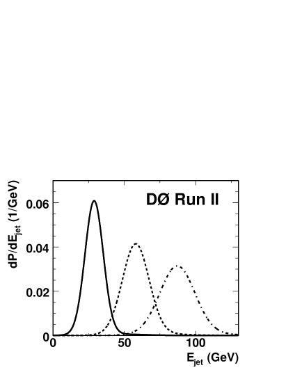
Abbildung 29: Jet energy transfer functions for light-quark jets in the D0 detector in the region $\left|\eta\right|<0.5$, for parton energies $E_{p}=30\ {\rm GeV}$ (solid), $60\ {\rm GeV}$ (dashed), and $90\ {\rm GeV}$ (dash-dotted curve). The parametrization corresponds to the reference jet energy scale, $JES=1.0$ [39].

8.4.4 Parametrization of the Muon Momentum Resolution

Only the D0 experiment so far considers the muon resolution explicitly in the likelihood calculation. To describe the resolution of the central tracking chamber, the resolution of the charge divided by the transverse momentum of a particle is considered as a function of pseudorapidity. The muon transfer function is parametrized as

$$W_{\mu}\left(\left(q/p_{T}\right)_{\mu}^{\rm rec},\left(q/p_{T}\right)_{\mu}^{\rm ass}\right)=\frac{1}{\sqrt{2\pi}\sigma}\exp\left(-\frac{1}{2}\left(\frac{\left(q/p_{T}\right)_{\mu}^{\rm rec}-\left(q/p_{T}\right)_{\mu}^{\rm ass}}{\sigma}\right)^{2}\right)\ ,$$ (36)

where $q$ denotes the charge and $p_{T}$ the transverse momentum assumed (ass) or reconstructed (rec) for a muon. The resolution

$$\sigma=\left\{\begin{array}[]{cc}\sigma_{0}&{\rm for}\ |\eta|\leq\eta_{0}\vspace{2ex}\\ \sqrt{\sigma_{0}^{2}+\left[c\left(|\eta|-\eta_{0}\right)\right]^{2}}&{\rm for}\ |\eta|>\eta_{0}\end{array}\right.$$ (37)

is obtained from muon tracks in simulated events. The muon charge is not used in the calculation of $L_{t\bar{t}}$ and $L_{\rm bkg}$; however, for muons with large transverse momentum the possibility of reconstruction of a track bent in the wrong direction is automatically taken into account in the transfer function when using this parametrization.

8.4.5 The Transfer Function for the Unclustered Transverse Momentum

The probability density to observe unclustered transverse momentum in the event is only used in the CDF dilepton analysis; it is parametrized as a Gaussian in each of the $x$ and $y$ directions, with no correlation.

8.5 The Signal Likelihood $L_{t\bar{t}}$

When spin correlations between the top and antitop quarks are neglected, the leading-order matrix element for the process $q\bar{q}\to t\bar{t}$ is given by [78]

$$|\mathscr{M}_{q\bar{q}\to t\bar{t}}|^{2}=\frac{g_{s}^{4}}{9}F\overline{F}\left(2-\beta^{2}s_{qt}^{2}\right)\ ,$$ (38)

where $g_{s}^{2}/(4\pi)=\alpha_{s}$ is the strong coupling constant, $\beta$ is the velocity of the top quarks in the $t\bar{t}$ rest frame, and $s_{qt}$ denotes the sine of the angle between the incoming parton and the outgoing top quark in the $t\bar{t}$ rest frame. If the top quark decay products include a leptonically decaying $W$ boson, while the antitop decay includes a hadronically decaying $W$, one has

$$F = \frac{g_{w}^{4}}{4}\left(\frac{m_{{b\ell\nu}}^{2}-m_{{\ell\nu}}^{2}}{\left(m_{{b\ell\nu}}^{2}-m_{t}^{2}\right)^{2}+\left(m_{t}\Gamma_{t}\right)^{2}}\right)\left(\frac{m_{{b\ell\nu}}^{2}\left(1-{\hat{c}}_{b\ell}^{2}\right)+m_{{\ell\nu}}^{2}\left(1+{\hat{c}}_{b\ell}\right)^{2}}{\left(m_{{\ell\nu}}^{2}-m_{W}^{2}\right)^{2}+\left(m_{W}\Gamma_{W}\right)^{2}}\right)\ ,$$ (39)

$$\overline{F} = \frac{g_{w}^{4}}{4}\left(\frac{m_{{\overline{b}d\overline{u}}}^{2}-m_{{d\overline{u}}}^{2}}{\left(m_{{\overline{b}d\overline{u}}}^{2}-m_{t}^{2}\right)^{2}+\left(m_{t}\Gamma_{t}\right)^{2}}\right)\left(\frac{m_{{\overline{b}d\overline{u}}}^{2}\left(1-{\hat{c}}_{\overline{b}d}^{2}\right)+m_{{d\overline{u}}}^{2}\left(1+{\hat{c}}_{\overline{b}d}\right)^{2}}{\left(m_{{d\overline{u}}}^{2}-m_{W}^{2}\right)^{2}+\left(m_{W}\Gamma_{W}\right)^{2}}\right)$$ (40)

(for the reverse case in $\ell$$+$jets events, replace $b\leftrightarrow\overline{b}$, $\ell\leftrightarrow d$, and $\nu\leftrightarrow\overline{u}$; for dilepton events, replace $d$ and $\overline{u}$ by the second charged lepton and neutrino, respectively). Here, $g_{w}$ denotes the weak charge ($G_{\rm F}/\sqrt{2}=g_{w}^{2}/8m_{W}^{2}$), $m_{t}$ and $m_{W}$ are the masses of the top quark (which is to be measured) and the $W$ boson, and $\Gamma_{t}$ and $\Gamma_{W}$ are their widths. Invariant top and $W$ masses in a particular event are denoted by $m_{xyz}$ and $m_{yz}$, respectively, where $x$, $y$, and $z$ are the decay products. The cosine of the angle between particles $x$ and $y$ in the $W$ rest frame is denoted by ${\hat{c}}_{xy}$. Here and in the following, the symbols $d$ and $\overline{u}$ stand for all possible decay products in a hadronic $W$ decay. The top quark width is given as a function of the top quark mass as [3]

$$\Gamma_{t}=\frac{G_{\rm F}m_{t}^{3}}{8\pi\sqrt{2}}\left(1-\frac{m_{W}^{2}}{m_{t}^{2}}\right)^{2}\left(1+2\frac{m_{W}^{2}}{m_{t}^{2}}\right)\left[1-\frac{2\alpha_{s}}{3\pi}\left(\frac{2\pi^{2}}{3}-\frac{5}{2}\right)\right]\ .$$ (41)

The correct association of reconstructed jets with the final-state quarks in Equations (39) and (40) is not known. Therefore, the transfer function takes into account all possible jet-parton assignments as described in Section 8.4. However, in the case of the signal likelihood for $\ell$$+$jets events, the mean value of the two assignments with the 4-momenta of the quarks from the hadronic $W$ decay interchanged may be computed explicitly by using the symmetrized formula

$$\overline{F} = \frac{g_{w}^{4}}{4}\left(\frac{m_{{\overline{b}d\overline{u}}}^{2}-m_{{d\overline{u}}}^{2}}{\left(m_{{\overline{b}d\overline{u}}}^{2}-m_{t}^{2}\right)^{2}+\left(m_{t}\Gamma_{t}\right)^{2}}\right)\left(\frac{m_{{\overline{b}d\overline{u}}}^{2}\left(1-{\hat{c}}_{\overline{b}d}^{2}\right)+m_{{d\overline{u}}}^{2}\left(1+{\hat{c}}_{\overline{b}d}^{2}\right)}{\left(m_{{d\overline{u}}}^{2}-m_{W}^{2}\right)^{2}+\left(m_{W}\Gamma_{W}\right)^{2}}\right)$$ (42)

instead of (40), where only the terms containing ${\hat{c}}_{\overline{b}d}$ are affected. Consequently, only a summation over half the jet-quark assignments remains to be evaluated.

The leading-order matrix element for the process $gg\to t\bar{t}$ is [57]

$$|\mathscr{M}_{gg\to t\bar{t}}|^{2}=g_{s}^{4}F\overline{F}\left(\frac{1}{6\tau_{1}\tau_{2}}-\frac{3}{8}\right)\left(\tau_{1}^{2}+\tau_{2}^{2}+\rho-\frac{\rho^{2}}{4\tau_{1}\tau_{2}}\right)\ ,$$ (43)

with

$$\tau_{i}=\frac{m_{g_{i}b\ell\nu}^{2}-m_{b\ell\nu}^{2}}{m_{b\ell\nu\overline{b}d\overline{u}}^{2}}\ {\rm and}\ \rho=\frac{4m_{t}^{2}}{m_{b\ell\nu\overline{b}d\overline{u}}^{2}}\ ,$$ (44)

where $g_{i}$, $i=1,2$ denotes the two incoming gluons. Here, again $t\bar{t}$ spin correlations have been neglected. This process is only taken into account explicitly in the CDF measurement based on the Dynamical Likelihood method. In the Matrix Element measurements it is not computed because the top and $W$ propagator and decay parts of the matrix element, which contain most of the information on the top quark mass and the separation of signal and background events, are identical.

The computation of the signal likelihood $L_{t\bar{t}}$ involves an integral over the momenta of the colliding partons and over 6-body phase space to cover all possible partonic final states, cf. Equation (8.3). The number of dimensions of the integration is reduced by the following conditions:

• The transverse momentum of the colliding partons is assumed to be zero, or to be consistent with the observed unclustered transverse energy (in the Dynamical Likelihood measurement). The transverse momentum of the $t\bar{t}$ system then follows from conservation of 4-momentum because the leading-order matrix element is used to describe $t\bar{t}$ production. Also, the $z$ momentum and energy of the $t\bar{t}$ system are known from the momenta of the colliding partons.

• The directions of the quarks and the charged lepton in the final state are assumed to be exactly measured.

• The energy of electrons from $W$ decay is assumed to be perfectly measured. The corresponding statement is not necessarily true for high momentum muons, and an integration over the muon momentum is performed in the D0 analysis.

Even after these considerations, a multi-dimensional integral remains to be calculated. In the Matrix Element analyses, this calculation is performed numerically with the Monte Carlo program vegas [79, 80].

8.6 The Background Likelihood

There are in general many background processes that can lead to an observed event. It is not problematic per se to not fully account for all backgrounds in the event likelihood; in fact, the Dynamical Likelihood measurements by CDF omit any explicit treatment of background in the likelihood. Because of the assumptions made in the Matrix Element technique, it is always necessary to calibrate the measurement technique with pseudo-experiments with varying input top quark masses, jet energy scales, and sample compositions as described in Section 10.2. An incomplete background likelihood will lead to a shift of the measured top quark mass value; this shift will in general depend on the top quark mass itself and on the fraction of events in the sample that are not accounted for in the overall likelihood. The shift is determined in the calibration procedure. When a background term is omitted in the event likelihood, the situation will thus be quantitatively, but not qualitatively different from that in an analysis that includes this term in the likelihood.

If several different background processes have similar kinematic characteristics, it is also possible to approximately describe the total background by the likelihood for only one of the background processes, multiplied by the total background fraction, cf. Equation (18). This technique has been applied by both CDF and D0 in the Matrix Element analyses in the $\ell$$+$jets channel, where a likelihood for QCD multijet production is not explicitly calculated. While this is a better approximation than not accounting for multijet background at all, it still has to be studied with pseudo-experiments and taken into account in the calibration. It should be noted that independently of the definition of the background likelihood used, any uncertainty in the characteristics of a background process has to be evaluated with pseudo-experiments and accounted for by a systematic error on the final measurement value, see Section 11.1.8.

Even if only leading-order background processes and only the most important among them are considered, it is not practical to explicitly evaluate all individual diagrams. Instead, routines from existing Monte Carlo generators are used to compute the likelihood for generic processes. They take into account the relative importance of the various subprocesses that contribute and perform a statistical sampling of all possible spin, flavor, and color configurations. Because the background likelihood does not depend on the top quark mass, it does not have to be computed for as many different assumptions as the signal likelihood and it is possible to evaluate the matrix elements without a dedicated routine optimized for speed.

The generic background process taken into account by both CDF and D0 for the Matrix Element analyses in the $\ell$$+$jets channel is the production of a leptonically decaying $W$ boson in association with four additional light partons, $W\!+\!{\rm\text{4}p}$. Events with a leptonically decaying $W$ boson and four partons that include heavy-flavor quarks are not considered separately because their kinematic characteristics are very similar to those of $W\!+\!{\rm\text{4}p}$ events. QCD multijet production, the second-largest background source, is not taken into account explicitly in the event likelihood.

The modeling of the $W\!+\!{\rm\text{4}p}$ process in the vecbos [81] generator is used to calculate the background likelihood $L_{\rm bkg}$. The jet directions and the charged lepton are taken as well-measured, also for muons in the D0 analysis. The integral over the quark energies in Equation (22) is performed by generating Monte Carlo events with parton energies distributed according to the jet transfer function. In these Monte Carlo events, the neutrino transverse momentum is given by the condition that the transverse momentum of the $W$$+$jets system be zero, while the invariant mass of the charged lepton and neutrino is assumed to be equal to the $W$ mass to obtain the neutrino $z$ momentum (both solutions are considered). The mean result from all 24 possible assignments of jets to quarks in the matrix element is calculated, and the mean over a number of Monte Carlo events is taken to be the $L_{\rm bkg}$ value. The calibration described in Section 10.2 supports that it is not necessary to compute $L_{\rm bkg}$ for different $JES$ values; only the value $L_{\rm bkg}\left(JES=1\right)$ is used.

The CDF Matrix Element measurement in the dilepton channel considers the following backgrounds explicitly in the event likelihood:

• a leptonically decaying $Z$ boson in association with two partons, $Z/\gamma^{*}$$+$2p,

• two leptonically decaying $W$ bosons in association with two partons, $WW$$+$2p (this contribution is negligible if a $b$-tagged jet is required and thus only considered in the topological analysis), and

• one leptonically decaying $W$ boson in association with three partons, one of which yields a jet that fakes an isolated charged lepton in the detector, $W$$+$3p.

Routines from the alpgen [20] generator are used to perform the statistical sampling to average the differential cross section. In the case of the $Z/\gamma^{*}$$+$2p process, in which no energetic neutrino occurs, the assumption of zero transverse momentum of the $Z/\gamma^{*}$$+$2p system is relaxed, and an integration over all possible values of $p_{T}$ is performed. For the $W$$+$3p process, it is assumed that the isolated lepton originating from the misidentified jet carries most of the jet energy (otherwise it would not appear isolated in the detector), and the jet energy transfer function is taken to relate it with the parton energy.

8.7 Normalization of the Likelihood for one Process

The likelihood for a process has to be normalized by the cross section $\sigma^{\rm obs}$ for observed events in the detector, as described in Equation (8.3). The cross section for observed events depends not only on the top quark mass (in the case of $L_{t\bar{t}}$), but via the jet $E_{T}$ requirements in the event selection also on the assumed value of the $JES$ parameter.

To normalize the signal likelihood in the D0 Matrix Element analysis, the integral $\sigma^{\rm obs}_{t\bar{t}}=\int{\rm d}\sigma_{t\bar{t}}(p\bar{p}\to x;\,m_{t},JES)f_{\rm acc}(x){\rm d}x$ has been computed as a function of $m_{t}$ and $JES$ as described in Equation (23). The results are shown in Figure 30 for $e$$+$jets and $\mu$$+$jets events as a function of $m_{t}$ for various choices of the $JES$ scale factor.

Abbildung 30: Cross section of observed $t\bar{t}$ events in the D0 detector [39] computed with the leading-order matrix element for (a) $e$$+$jets and (b) $\mu$$+$jets events as a function of the top quark mass $m_{t}$ for different choices of the $JES$ scale factor: $JES=1.12$ (dash-dotted), $JES=1.0$ (solid), and $JES=0.88$ (dotted lines). The branching fraction $t\bar{t}\to b\bar{b}\ell\nu q\bar{q}^{\prime}$ is not included, as such a constant overall scale factor is irrelevant for the analysis.

The normalization of the background likelihoods can in principle be determined in the same way. The computation of the integral in Equation (23) would be very computing intensive even though the dependence of $L_{\rm bkg}$ on the $JES$ parameter does not have to be taken into account as shown in the D0 analysis. The D0 experiment has therefore used a different method to compute the relative normalization of signal and background likelihoods (an overall scale factor is irrelevant in the analysis), assuming the relative contributions of the individual background subprocesses to the total background likelihood are known. This approach makes use of the fact that the fitted signal fraction $f_{t\bar{t}}$ of the sample will be underestimated if the background likelihood $L_{\rm bkg}$ is too large and vice versa. The relative normalization can therefore be adjusted until the signal fraction is determined correctly in pseudo-experiments of simulated events. Note that this technique can only be used when the $f_{t\bar{t}}$ parameter is left free in the fit (i.e. when no constraint from the $t\bar{t}$ and background cross section is used), as is the case for the CDF and D0 Matrix Element measurements in the $\ell$$+$jets channel. The calibration of the $f_{t\bar{t}}$ fit result is further discussed in Section 10.2.

9 The Ideogram Measurement Method

This section describes the Ideogram method and its application in top quark mass measurements. Like the Matrix Element and Dynamical Likelihood techniques discussed in the previous section, this method is based on a per-event likelihood that depends on the top quark mass. The signal and background likelihoods are however only based on the reconstructed top quark and $W$ boson masses in each event and do not make use of the full kinematic information. This means that the amount of computation time needed for the analysis is reduced significantly.

The Ideogram method has previously been used to measure the $W$ boson mass at the DELPHI experiment at LEP [82]. It is now also applied by the D0 and CDF experiments to measure the top quark mass using $t\bar{t}$ events in the $\ell$$+$jets [83] and all-jets channels [58], respectively. In Section 9.1, the event selection and reconstruction using a kinematic fit are summarized for these two analyses. The definition of the event likelihood in the Ideogram method is then discussed in Section 9.2 and compared with the approach in the Matrix Element and Dynamical Likelihood methods.

9.1 Event Selection and Kinematic Reconstruction

The event selection in the D0 $\ell$$+$jets analysis is identical to the one used in the Matrix Element measurement described in Section 8.1, except that events are also used if more than four jets are reconstructed (only the four highest-$E_{T}$ jets are used to measure the top quark mass). There is an additional cut on the $\chi^{2}$ obtained from a kinematic fit as described below.

The kinematic requirements on the events in the CDF measurement in the all-jets channel are similar to those described in Section 7.3. The most important requirements are:

• no significant missing transverse energy,

• removal of events with a charged lepton with high $p_{T}$,

• events must contain between 6 and 8 jets within $|\eta|<2.0$ with $E_{T}>15\,\,\mathrm{Ge\kern-1.00006ptV}$, and

• the sum of jet transverse energies must satisfy $\sum_{\rm jets}E_{T}>280\,\,\mathrm{Ge\kern-1.00006ptV}$.

There are additional event quality cuts and requirements on the event shape using the aplanarity and centrality.

The events are then subjected to a kinematic fit constraining them to the $t\bar{t}$ hypothesis. In the D0 $\ell$$+$jets analysis, the kinematic fit is similar to the one described in Section 7.1, yielding one fitted top quark mass $m_{t}^{i}$, the corresponding uncertainty $\sigma_{m_{t}}^{i}$ and the best $\chi^{2}_{i}$ for each of the 12 different jet-parton assignments (an interchange of the two jets assumed to come from the hadronic $W$ decay does not change the kinematic fit) and for each of the two possible solutions for the longitudinal neutrino momentum component $p_{\nu,z}$. The index $i$ thus runs over 24 different possibilities. All of these values depend on the assumed value $JES$ of the jet energy scale.

The kinematic fit in the all-jets case is identical to the one discussed in Section 7.3 except that in this analysis, the masses of the two decaying top quarks per event are treated as independent fit parameters. Thus, for each of the 90 jet-parton assignments $i$ that have to be distinguished in an event, the two fitted top quark masses $m_{t}^{i,\,1/2}$ and their uncertainties $\sigma_{m_{t}}^{i,\,1/2}$ are determined together with the minimum $\chi^{2}_{i}$. In the analysis in the all-jets channel, no in situ calibration of the jet energy scale is performed so far.

9.2 The Event Likelihood

The definition of the likelihood $L_{\rm evt}$ to observe a given selected event is identical to that used in the Matrix Element method, cf. Section 8.2:

$$L_{\rm evt}\left(x;\,m_{t},JES,f_{t\bar{t}}\right)=f_{t\bar{t}}L_{t\bar{t}}\left(x;\,m_{t},JES\right)+\left(1-f_{t\bar{t}}\right)L_{\rm bkg}\left(x;\,JES\right)\ ,$$ (45)

where $L_{t\bar{t}}$ and $L_{\rm bkg}$ are the likelihoods to observe the event if it was produced via the signal or any of the background processes, respectively, $f_{t\bar{t}}$ is the overall fraction of signal events in the selected event sample, $x$ denotes the event observables, and $m_{t}$ and $JES$ are the assumed values of the top quark mass and jet energy scale which are to be measured (in the all-jets analysis, the parameter $JES$ is fixed to 1.0). The evaluation of the signal and background likelihoods however differs from that in the Matrix Element method.

The event observables can be classified into the kinematic information $x_{\rm kin}$ used in the kinematic fit to reconstruct the top quark mass and other variables $x_{{\rm topo/}b}$ (describing the event topology and the $b$-tagging information) that are uncorrelated with the top quark mass and used to improve the separation of signal and background events. The likelihood for the event to be produced via process $i$ can then in general be written as the product

$$L_{P}\left(x;\,m_{t},JES\right)=L_{P}^{\rm kin}\left(x_{\rm kin};\,m_{t},JES\right)L_{P}^{{\rm topo/}b}\left(x_{{\rm topo/}b}\right)\ ,$$ (46)

where the dependence on $m_{t}$ only enters for the signal process, $P=t\bar{t}$. The second term is only included in the D0 analysis. It recovers some of the topological information of the event (like the relative angles between the decay products) that can otherwise only be used in the Matrix Element method, while the $L_{P}^{\rm kin}$ term in the Ideogram method extracts information on $m_{t}$ only from invariant mass information obtained in the kinematic fit (which in turn is also insensitive to angular information). In addition, event quality and $b$-tagging information can be included in $L_{P}^{{\rm topo/}b}$. The kinematic and topological terms in the likelihood are discussed in turn in the following sections.

9.2.1 The Kinematic Likelihood for a Process

The kinematic part of the signal or background likelihood is calculated as a sum over all jet-parton assignments (and neutrino solutions, in the case of the $\ell$$+$jets analysis). The relative likelihood $w_{i}$ of assignment/solution $i$ to be correct is obtained from the minimum $\chi^{2}_{i}$ of the corresponding fit and from $b$-tagging information as

$$w_{i}\left(x_{\rm kin}^{i};m_{t},JES\right)=\exp\left(-\frac{1}{2}\left(\chi^{2}\right)^{i}\right)\prod_{j=1}^{n_{j}}W_{b}\left({\cal B}_{{\rm jet}\,j}^{\,\rm rec},\ \phi_{{\rm parton}\,k}^{\,\rm ass}\right)\ ,$$ (47)

where the product runs over all $n_{j}$ jets in the event, and $W_{b}$ is given by the $b$-tagging efficiencies for light and $b$-quark jets as defined in Equation (29). The weights depend on the top quark mass and jet energy scale because the results of the kinematic fit do (including the minimum $\chi^{2}$).

The kinematic term in the signal likelihood $L_{t\bar{t}}^{\rm kin}$ describes the correct jet-parton assignment (“$\rm ca$”) and all other assignments (“$\rm wa$”) separately and can be written as

$$L_{t\bar{t}}^{\rm kin}\left(x_{\rm kin};\,m_{t},JES\right)=\sum_{i}w_{i}\left(x_{\rm kin}^{i};m_{t},JES\right)[\phantom{\ +}\!\! \!\!f_{\rm ca}\!\! \!\!S_{\rm ca}\left(x_{\rm kin}^{i};m_{t},JES\right)$$

$$\ +\!\! \!\!\left(1-f_{\rm ca}\right)\!\! \!\!S_{\rm wa}\left(x_{\rm kin}^{i};m_{t},JES\right)]\ ,$$ (48)

where $i$ runs over all 24 assignments/solutions, and $f_{\rm ca}$ corresponds to the relative weight given to the correct assignment by the weights $w_{i}$. In the D0 analysis in the $\ell$$+$jets channel, the value of $f_{\rm ca}$ is determined from the simulation as the average fraction of weights $w_{\rm ca}/\left(\sum_{i}w_{i}\right)$ given to the correct assignment; the dependence of $f_{\rm ca}$ on the total number of reconstructed jets and the number of $b$-tagged jets is taken into account.

For the correct assignment, the likelihood to observe the fitted top quark mass $m_{t}^{\rm fit}$ takes into account both the natural width $\Gamma_{t}$ of the top quark and the experimental resolution $\sigma_{m_{t}}^{\rm fit}$, which is assumed to be Gaussian and determined on an event-by-event basis in the kinematic fit. The likelihood is given by their convolution

$$S_{\rm ca}\left(x_{\rm kin}^{i};m_{t},JES\right)=\int_{m^{\prime}}G\left(m_{t}^{{\rm fit},\,i},m^{\prime},\sigma_{m_{t}}^{{\rm fit},\,i}\right)BW(m^{\prime},m_{t}){\rm d}m^{\prime}\ ,$$ (49)

where the integration is over the true mass $m^{\prime}$ of the top quark in the given event. The Gaussian resolution $G$ and the relativistic Breit-Wigner $BW$ can be expressed as

$$G\left(m_{t}^{{\rm fit},\,i},m^{\prime},\sigma_{m_{t}}^{{\rm fit},\,i}\right) = \frac{1}{\sqrt{2\pi}\ \sigma_{m_{t}}^{{\rm fit},\,i}}\exp\left(-\frac{1}{2}\left(\frac{m_{t}^{{\rm fit},\,i}-m^{\prime}}{\sigma_{m_{t}}^{{\rm fit},\,i}}\right)^{2}\right)\ {\rm and}$$ (50)

$$BW(m^{\prime},m_{t}) = \frac{1}{\pi}\frac{m_{t}\Gamma_{t}}{\left(m^{\prime 2}-m_{t}^{2}\right)^{2}+m_{t}^{2}\Gamma_{t}^{2}}\ ,$$ (51)

respectively. The likelihood is sensitive to the jet energy scale via the $\chi^{2}$ obtained in the kinematic fit since a constraint to the known $W$ boson mass is applied. In the $\ell$$+$jets analysis, with only one fitted mass $m_{t}^{{\rm fit},\,i}$ per jet-parton assignment $i$, $m^{\prime}$ can be interpreted as the average of the top and antitop quark masses. In the analysis in the all-jets channel, the term $S_{\rm ca}$ contains one integral as given in Equation (49) for each of the two fitted masses.

Wrong jet-parton assignments in signal $t\bar{t}$ events cannot easily be described as a similar convolution. Therefore, the corresponding term $S_{\rm wa}\left(x_{\rm kin}^{i};m_{t},JES\right)$ is given by the distribution of fitted masses $m_{t}^{\rm fit}$ in simulated $t\bar{t}$ events, where the two neutrino solutions for the correct jet-parton assignment are excluded and all other assignments/solutions are weighted with $w_{i}$. Even though it describes wrong assignments, $S_{\rm wa}$ still depends on the top quark mass. The fitted uncertainty $\sigma_{m_{t}}^{\rm fit}$ is not used. In some simulated events, the correct jet-parton assignment cannot be unambiguously identified. These events are excluded when determining the shape of $S_{\rm wa}$; the calibration of the measurement technique is however performed using the full simulation including these events, as described in general in Section 10.2, so that the final measurement result is unbiased.

In both the $\ell$$+$jets and all-jets channels, background is described with one likelihood $L_{\rm bkg}$. The kinematic term of the background likelihood is given by

$$L_{\rm bkg}^{\rm kin}(x_{\rm kin};\,JES)=\sum_{i}w_{i}B(x_{\rm kin}^{i};\,JES)$$ (52)

with a weight $w_{i}$ per jet-parton assignment/solution $i$ as defined above in Equation (47). In the $\ell$$+$jets analysis, $B$ is the shape of the mass spectrum obtained in simulated $W\!+\!{\rm\text{4}p}$ events, where each assignment $i$ enters with its weight $w_{i}$ as in the likelihood. The shape $B$ of the background spectrum does not depend strongly on $JES$ (the number of background events does, but this is not relevant since the signal fraction $f_{t\bar{t}}$ is a free parameter in the measurement), and $L_{\rm bkg}^{\rm kin}$ is always evaluated at $JES=1$ like in the Matrix Element analyses, see Section 8.6.

In the all-jets channel, background is described by a mixture of $b\bar{b}\!+\!{\rm\text{4}p}$ events simulated with alpgen and $\rm 6p$ events obtained from the data. Here, $B$ is a two-dimensional function of the two fitted masses. As above, it is obtained as the weighted spectrum obtained in the background events. No $JES$ dependence is included in the likelihood since the $JES$ parameter is not fitted.

9.2.2 The Topological Likelihood for a Process

In the D0 analysis in the $\ell$$+$jets channel, a term $L_{i}^{{\rm topo/}b}$ is included in the likelihood that captures the information from the event topology, the event quality, and the number of $b$-tagged jets in the event. Note that in the kinematic term of the signal likelihood, $b$-tagging information is included to improve the identification of the correct jet-parton assignment in signal events, while it is used here to improve the separation between signal and background. The inputs used in the calculation are:

• Topological information: Four variables are used. These are

  • the missing transverse energy $E\kern-6.00006pt/_{T}$;

  • the aplanarity ${\cal A}$ as defined in Section 7.3, computed from the momenta of all jets and the leptonically decaying $W$ boson reconstructed in the kinematic fit;

  • the ratio $H_{T2}^{\prime}$ of the scalar sum of the jet transverse momenta, excluding the highest-$p_{T}$ jet, and the scalar sum of the longitudinal momenta of the jets and the reconstructed leptonically decaying $W$ boson; and

  • the quantity

    $$K_{T,{\rm min}^{\prime}}=\frac{\min\left(\Delta{\cal R}_{ij}\right)\min\left(E_{T,i},E_{T,j}\right)}{E_{T,W}}\ ,$$ (53)

    where $\min\left(\Delta{\cal R}_{ij}\right)$ is the minimum distance between any two jets among the four highest-$p_{T}$ jets.

  Although other variables like the scalar sum of all jet transverse momenta have better separation power between signal and background, these variables are correlated with the top quark mass, which is why they are not used in the topological likelihood. The separation obtained with these topological variables is shown in Figures 31(a) and (d).

• Fraction of track $p_{T}$ contained in jets: Considering scalar sums of track transverse momenta, this variable is defined as the fraction of track $p_{T}$ contained within the reconstructed jets of the event (i.e. within $\Delta{\cal R}<0.5$ of the calorimeter jet axes). This variable distinguishes clean events from events with poorly defined jets and is uncorrelated with the topological information described above. It provides separation in particular between $t\bar{t}$ and QCD multijet background events, as can be seen in Figures 31(b) and (e).

• $b$-tagging information: Finally, the number of $b$-tagged jets in the event is used as an input to the likelihood.

A likelihood discriminant $D$ is created from all input variables. The topological/$b$-tagging terms $L_{t\bar{t}}^{{\rm topo/}b}\left(x_{{\rm topo/}b}\right)$ and $L_{\rm bkg}^{{\rm topo/}b}\left(x_{{\rm topo/}b}\right)$ of the likelihood are then given by the fraction of signal or background events at the value of $D$ reconstructed for a particular event. These are shown in Figures 31(c) and (f). Note that while topological and $b$-tagging information are also used in the Matrix Element analysis, the $p_{T}$ fraction variable is unique to the Ideogram analysis.

Abbildung 31: D0 $\ell$$+$jets Ideogram measurement: Topological likelihood for $e$$+$jets (upper plots) and $\mu$$+$jets (lower plots) events. Plots (a) and (d) show the separation between $t\bar{t}$ signal (red), $W$$+$jets background (yellow), and QCD multijet background (blue) when only topological information is used. In plots (b) and (e), information from the track $p_{T}$ fraction contained in jets is included. Plots (a), (b), (d), and (e) show the expected distributions on an arbitrary linear vertical scale. Plots (c) and (f) show the final distributions used to compute the topological likelihood, which also include $b$-tagging information. In these plots, the expectations are scaled to the results from $425\,\,\rm pb^{-1}$ of data, which are are overlaid [83]. In all plots, the $t\bar{t}$ and $W$$+$jets predictions are from simulated events, while the QCD multijet distribution has been obtained from data using a signal depleted sample.

10 The Top Quark Mass Fit and its Calibration

With the methods presented in Sections 7, 8, and 9, a likelihood for a sample of selected events to be consistent with a given top quark mass hypothesis can be computed. This section describes how this information is used to determine the measurement value of the top quark mass and its (statistical) uncertainty. The calibration of the measurement method with simulated experiments is also discussed.

The previous sections describe how the likelihood as a function of the top quark mass hypothesis to obtain the observed data sample can be determined: via the comparison of the estimator distributions in data and simulation (template method, cf. Section 7), or using likelihoods calculated for each individual event with the Matrix Element (Section 8) or Ideogram methods (Section 9). Section 10.1 describes the step of obtaining a (raw) measurement value of the top quark mass and its statistical uncertainty from this information.

This (raw) measurement value is only correct if the assumptions made to derive it reflect reality. Uncertainties on these assumptions will translate into systematic uncertainties on the measurement, as described in Section 11. On the other hand, known deficiencies or approximations in the technique used to determine the likelihoods can be corrected for by calibrating the measurement with fully simulated events. This step also allows for a test of the uncertainties obtained in the fitting procedure and a comparison of the measured uncertainty in data with expectations. It is further described in Section 10.2.

10.1 The Fitting Procedure

The technical details of how a (raw) measurement of the top quark mass is extracted from the likelihood information varies between the individual analyses. For example, the procedure depends on whether the likelihood is known for arbitrary top quark masses or only for a discrete set of values. Furthermore, some analyses require the simultaneous measurement of the top quark mass and jet energy scale.

To cover the techniques applied, the fitting procedures used in the CDF template measurement in the $\ell$$+$jets channel [38, 7] and in the D0 Matrix Element measurement in the $\ell$$+$jets channel [39] are described as examples in Sections 10.1.1 and 10.1.2, respectively. The fitting procedure does not depend a priori on the $t\bar{t}$ event topology.

10.1.1 Fitting Procedure in the CDF Lepton+Jets Template Analysis

This section describes the fit used in the CDF template analysis in the $\ell$$+$jets channel to determine the top quark mass $m_{t}$ and the jet energy scale $JES$ (as well as the signal fraction).

The event selection, estimators, and template parametrizations are described in Section 7.1 and are briefly recapitulated here:

• The selected events are grouped into four categories with different expected signal to background ratio depending on the number and transverse energies of $b$-tagged jets in the event.

• The top quark mass $m_{t}^{\rm reco}$ obtained in a kinematic fit of each measured event to the $t\bar{t}$ hypothesis is used as estimator for the top quark mass; the dijet mass $\mathrm{m}_{jj}$ is taken as estimator for the jet energy scale whose deviation $\Delta_{JES}$ from the standard scale is measured in units of its uncertainty $\sigma_{c}$.

• For signal $t\bar{t}$ events, the $m_{t}^{\rm reco}$ templates are parametrized as functions of $m_{t}^{\rm reco}$ as well as of the true top quark mass $m_{t}$; similarly the $\mathrm{m}_{jj}$ templates are parametrized as functions of $\mathrm{m}_{jj}$ and the parameter $\Delta_{JES}$ to be measured. The background templates are parametrized as functions of $m_{t}^{\rm reco}$ and $\mathrm{m}_{jj}$, too.

The $m_{t}^{\rm reco}$ and $m_{jj}$ values in the data events are compared to the signal and background templates in an unbinned likelihood fit, which determines the top quark mass, jet energy scale, and the number of signal and background events in each of the four event categories. The likelihood for one event category is computed as the product of likelihoods for each data event, which in turn contain four terms each:

• the likelihood to measure the reconstructed value of $m_{t}^{\rm reco}$, obtained from the linear combination of signal and background $m_{t}^{\rm reco}$ templates for given $m_{t}$ and $\Delta_{\rm JES}$ hypotheses, with relative contributions of signal and background also determined in the fit (mainly sensitive to $m_{t}$);

• a similar term based on $m_{jj}$ (mainly sensitive to $\Delta_{\rm JES}$);

• a term describing the probability of having certain numbers of signal and background events in the data, given the total number of selected events; and

• a constraint on the expected number of background events (not for the 0-tag event category).

The likelihoods for all four event categories are then multiplied, and a constraint to the a priori knowledge of the jet energy scale is included as another overall factor. Since the $m_{t}$ and $\Delta_{\rm JES}$ parameters are the same in all event categories, a total of ten parameters are determined in the fit. These parameters are determined simultaneously using minuit [84].

10.1.2 Fitting Procedure in the D0 Lepton+Jets Matrix Element Analysis

In an analysis with parametrized templates, it is possible to let the minimization program (e.g. minuit) decide for which assumed parameter values to evaluate the overall likelihood. This is impractical for the Matrix Element and Ideogram methods, where the calculation of the overall likelihood for one hypothesis is a time-consuming process. In these analyses, a different approach is therefore followed:

• In a first step, the overall likelihood is calculated for each hypothesis in a grid of assumed parameter values.

• Second, the dependency of the likelihood on the parameters that are to be measured is fitted with a function.

• The minimum of this function yields the central measurement value, and the statistical uncertainty is given by the $68\%$ confidence region around this central value.

As an example, the fitting procedure used in the D0 Matrix Element measurement in the $\ell$$+$jets channel is described here.

Also in this analysis a simultaneous measurement of the top quark mass $m_{t}$, jet energy scale $JES$, and signal fraction $f_{t\bar{t}}$ is performed. For each selected event, the signal likelihood is evaluated for a grid of assumed $m_{t}$ and $JES$ values in steps of $2.5\,\,\mathrm{Ge\kern-1.00006ptV}$ and $0.01$. The background likelihood is calculated for $JES=1$ only and is assumed not to depend on the $JES$ parameter value.

For any given ($m_{t}$, $JES$) assumption, the likelihood as a function of $f_{t\bar{t}}$ can then be calculated easily as the linear combination given in Equation (18). The signal fraction $f_{t\bar{t}}^{\rm best}$ that maximizes the overall likelihood is calculated for each ($m_{t}$, $JES$) parameter pair, and the likelihood value corresponding to this value is used in further computations. The overall result quoted for the fitted signal fraction $f_{t\bar{t}}$ is derived from the value obtained at the ($m_{t}$,$JES$) point in the grid with the maximum likelihood value for the event sample. The uncertainty on $f_{t\bar{t}}$ is computed by varying $f_{t\bar{t}}$ at fixed $m_{t}$ and $JES$ until $\Delta(-\ln L)=+\frac{1}{2}$. This uncertainty does not account for correlations between $f_{t\bar{t}}$, $m_{t}$, and $JES$.

The result for the top quark mass is obtained from a projection of the two-dimensional grid of likelihood values onto the $m_{t}$ axis. In this projection, correlations are taken into account. The likelihood for a given $m_{t}$ hypothesis is obtained as the integral over the likelihood as a function of $JES$, using linear interpolation between the grid points and Gaussian extrapolation to account for the tails for $JES$ values outside the range considered in the grid.

The likelihoods as a function of assumed top quark mass are converted to $-\ln L$ values. These $-\ln L$ points are then fitted with a fourth order polynomial in the region defined by the condition $\Delta\ln L<3$ around the best value. The $m_{t}$ value that maximizes the fitted likelihood is taken to be the measured value of the top quark mass. The lower and upper uncertainties on the top quark mass are defined such that 68% of the total likelihood integral is enclosed by the corresponding top quark mass values, with equal likelihood values at both limits of the 68% confidence level region. The same projection and fitting procedure is applied to determine the value of the $JES$ parameter.

The inclusion of $b$-tagging information introduces two significant improvements to the analysis: Both the separation between signal and background and the identification of the correct jet-parton assignment (under the signal hypothesis) are improved. Since the signal and background likelihoods are evaluated on an event-by-event basis and the $b$-tagging information is encoded in the transfer function (cf. Section 8.4), both aspects are in principle addressed, and it should not be necessary to divide the event sample into subsamples of different purity like in the template analysis described in Section 10.1.1. Nevertheless, the D0 experiment has taken a different approach. The transfer function $W(x,y;\,JES)$ given in Equation (8.4.1) is modified to obtain

$$\tilde{W}(x,y;\,JES)=\frac{W(x,y;\,JES)}{\displaystyle\sum_{i=1}^{n_{\rm comb}}\prod_{j=1}^{n_{j}}W_{b}\left({\cal B}_{{\rm jet}\,j}^{\,\rm rec},\ \phi_{{\rm parton}\,k}^{\,\rm ass}\right)}\ .$$ (54)

This new transfer function is used in the computation of the signal likelihood so that the $L_{t\bar{t}}$ values can be compared with those of the background likelihood, which in turn are computed without taking $b$-tagging information into account at all, i.e. with the transfer function given in Equation (8.4.1).

This method implies that only the identification of the correct jet-parton assignment in $t\bar{t}$ events is improved. To recover the enhanced separation of signal and background events, the event sample is subdivided into three categories based on the number of $b$-tagged jets per event. Overall values of the top quark mass $m_{t}$, jet energy scale $JES$, and signal fraction $f_{t\bar{t}}$ are determined for all three categories together by relating the sample composition in each category to the overall signal fraction. It should be possible in future updates of the measurement to use the full transfer function for the background likelihood and thus avoid fitting different subsamples of events.

10.2 Validation and Calibration of the Measurement

If the model used to describe the data is correct, then the measurement method should yield unbiased results and the correct statistical uncertainty. To validate the measurement technique, this assumption can be verified with simulated pseudo-experiments using events that have been generated with this model.

However, most analysis techniques involve some simplifications, for example via the template parametrization or the simplified treatment of detector resolution and physics processes in the Matrix Element and Ideogram methods. Given these simplifications, it cannot be assumed that every aspect of the data is accounted for. To calibrate the measurement, it is first essential that the agreement between data and the full simulation is verified. Monte Carlo events generated with the full simulation are then used to compose pseudo-experiments for the calibration.

The following information is obtained from pseudo-experiments:

• The relation between the expected (mean) raw measurement value $\langle m_{t}^{raw}\rangle$ and the true input value $m_{t}$. Because the mass range of interest is limited a priori to a range around a value $m_{t}^{0}$, it is usually parametrized as a linear function in $m_{t}$ as

  $$\left\langle m_{t}^{raw}\right\rangle=m_{t}^{0}+s\left(m_{t}-m_{t}^{0}\right)+o\,.$$ (55)

  The symbols $s$ and $o$ stand for the slope of the calibration curve and for the offset at mass $m_{t}^{0}$.

• The width $w$ of the pull distribution. To test that the fitted uncertainties describe the actual measurement uncertainty, the deviation of the measurement value from the true value is divided by the fitted measurement uncertainty in each pseudo-experiment. The width of this distribution of deviations normalized by the measurement uncertainty is referred to as pull width.

• The expected distribution of measurement uncertainties.

This information can be determined accordingly for any other parameter that is measured ($JES$ and $f_{t\bar{t}}$, if applicable). In the validation step, values of $s=1$, $o=0$, and $w=1$ are expected. Because of simplifications in the measurement technique, this is in general not true for the calibration based on the full simulation. The values of $s$ and $o$ obtained in the calibration are used to correct the raw measurement value, and the measurement uncertainty is adjusted according to the value of $w$. As an example, the results from the validation and calibration of the D0 measurement with the Matrix Element method in the $\ell$$+$jets channel are described in the following paragraphs.

Validation:

To validate the Matrix Element method, the D0 collaboration has generated events with leading-order event generators (madgraph [85] for $t\bar{t}$ events and alpgen for $W$$+$jets events), i.e. not including initial- or final-state radiation, for various values of the top quark mass and jet energy scale. These events have been smeared according to the transfer function described in Section 8.4. The events are required to pass a simplified kinematic selection similar to the actual event selection, and the normalization of the likelihood is determined for this selection according to Equation (23).

Pseudo-experiments are composed of these events with the number of signal and background events as observed in the data, and the measurement values $m_{t}$ and $JES$ are determined for each pseudo-experiment. In a test where $b$-tagging information is not used (jets are assumed not to be $b$-tagged), the fitted top quark mass and jet energy scale are unbiased within statistical uncertainties of the test of $300\,\,\mathrm{Me\kern-1.00006ptV}$ and $0.003$, respectively. Furthermore, the fitted $m_{t}$ value does not depend on the input $JES$ value used in the generation of the pseudo-experiments, and similarly, the fitted $JES$ value is independent of the true input top quark mass. The pull width is in agreement with $1.0$. This validation study and its results are described in detail in [86].

Calibration:

For the calibration, fully simulated $t\bar{t}$ and $W$$+$jets events are used to compose pseudo-experiments with the same numbers of events as measured in the data. As an example, the calibration curves for the top quark mass and jet energy scale in the D0 Matrix Element measurement (including $b$-tagging information) are shown in Figures 32 and 33. The deviation between input and fitted jet energy scale arises from the simplified description of the detector response. Given this offset, the (anti-)correlation between the top quark mass and jet energy scale measurements explains the observed shift between true and fitted $m_{t}$. The widths of the pull distributions are slightly larger than one.

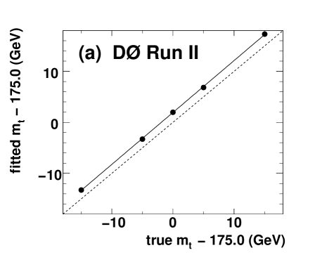
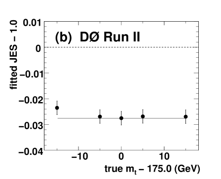
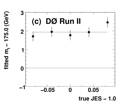
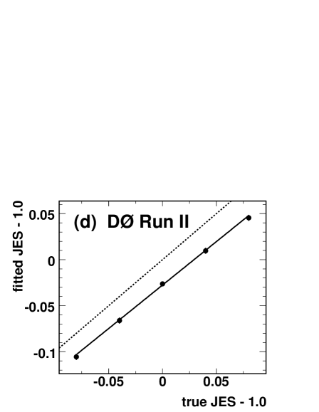
Abbildung 32: Calibration of the fitting procedure in the D0 Matrix Element analysis in the $\ell$$+$jets channel [39]. The upper plots show the reconstructed top quark mass (a) and the measured jet energy scale (b) as a function of the input top quark mass. The two lower plots show the reconstructed top quark mass (c) and the measured jet energy scale (d) as a function of the input jet energy scale. The solid lines show the results of linear fits to the points, which are used to calibrate the measurement technique. The dashed lines would be obtained for equal fitted and true values of $m_{t}$ and $JES$.

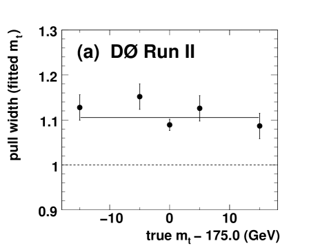
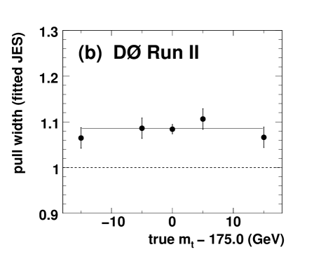
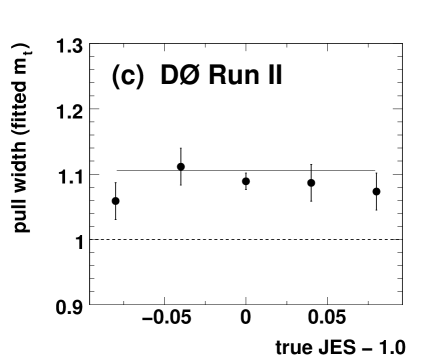
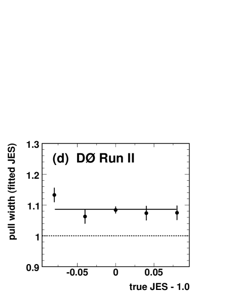
Abbildung 33: Calibration of the fitting procedure in the D0 Matrix Element analysis in the $\ell$$+$jets channel [39]. The upper plots show the widths of the pull distributions for the top quark mass (a) and jet energy scale (b) as a function of the input top quark mass. The two lower plots show the widths of the pull distributions for the top quark mass (c) and jet energy scale (d) as a function of the input jet energy scale. The solid lines show the mean pull width, while the dashed lines indicate a pull width of $1.0$.

For each pseudo-experiment, the statistical uncertainty on the top quark mass is multiplied by the pull width, and the resulting distribution of statistical uncertainties is shown in Figure 34. This allows a comparison with the statistical uncertainty obtained in the data, which is also shown in the figure.

The interpretation of such a comparison is not as straightforward as it may seem: The pseudo-experiments have always been composed with the same expected numbers of signal and background events. These numbers have been obtained from the data using a topological likelihood fit independent of the Matrix Element method; it yields the $t\bar{t}$ fraction of the sample with an (absolute) error of 7% for $0.4\,\,\rm fb^{-1}$ of data (the $f_{t\bar{t}}$ result from the Matrix Element method itself has a similar uncertainty). If this uncertainty is also taken into account, what at first glance appears to be a discrepancy between the fitted top quark mass and jet energy scale uncertainties in the data and the expectation becomes much more consistent. This is shown in Figure 35, where the expected uncertainties for a combined $m_{t}$ and $JES$ fit using topological information only (i.e., no $b$-tagging information) are shown for two types of pseudo-experiments: Experiments with a sample composition according to the central measured value; and experiments with $f_{t\bar{t}}$ varied down by one standard deviation. Much better agreement between predicted and observed uncertainties is obtained with the latter class of pseudo-experiments.

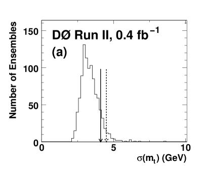
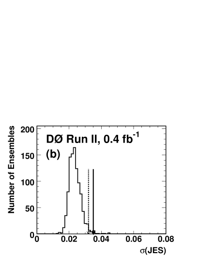
Abbildung 34: Test of the uncertainties on (a) $m_{t}$ and (b) $JES$ obtained in the D0 Matrix Element analysis [39]. The distributions of fitted uncertainties obtained from pseudo-experiments are shown by the histograms. The histograms show the combined distributions of upper and lower uncertainties as the individual distributions are very similar. The upper and lower uncertainties observed in the data are indicated by the solid and dashed arrows, respectively.

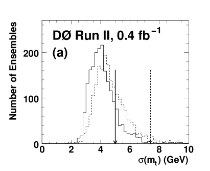
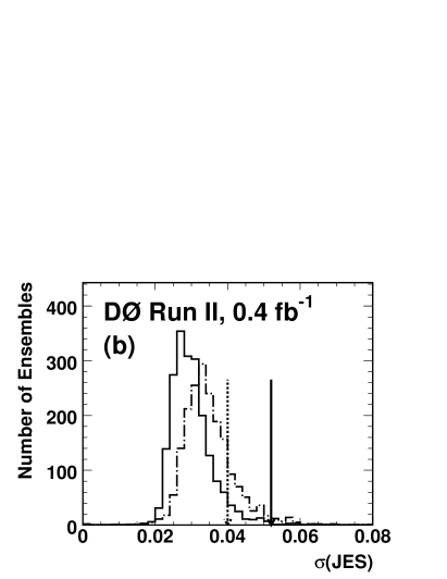
Abbildung 35: D0 Matrix Element analysis in the $\ell$$+$jets channel: Effect of the $t\bar{t}$ fraction $f_{t\bar{t}}$ on the expected fit uncertainties. The uncertainties on (a) $m_{t}$ and (b) $JES$ obtained by D0 in the topological Matrix Element analysis when a sample composition according to the central $f_{t\bar{t}}$ value is assumed is shown by the solid histogram [39]. Pseudo-experiments with $f_{t\bar{t}}$ varied down by one standard deviation yield the distributions of uncertainties shown by the dash-dotted histogram. The upper and lower uncertainties observed in the data are indicated by the solid and dashed arrows, respectively.

The $f_{t\bar{t}}$ calibration curve for the CDF Matrix Element analysis in the $\ell$$+$jets channel is shown in Figure 36. The raw value $f_{t\bar{t}}^{raw}$ is smaller than the true value. This is due to the fact that a leading-order matrix element is used to describe the $t\bar{t}$ process, while higher-order effects are included in the full simulation: In the simulation, about $20-30\,\%$ of $t\bar{t}$ events have jets and partons that cannot be unambiguously matched, i.e. at least one of the four reconstructed jets cannot be assigned to a parton from the $t\bar{t}$ decay. These events yield poor top quark mass information and degrade the uncertainty estimate of the likelihood fit. Figure 37 shows a D0 study which illustrates that jet-parton matched $t\bar{t}$ events tend to have a higher signal than background likelihood, which is how the mass fit identifies them as signal-like. There is no such separation for signal events in which one or more jets cannot be matched to a parton, so that these events contribute much less mass information to the final likelihood.

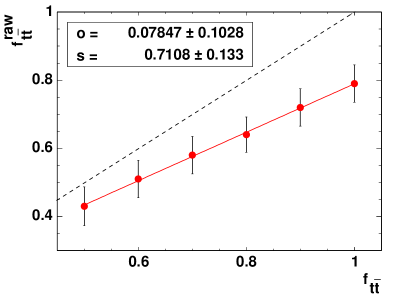
Abbildung 36: Calibration of the $f_{t\bar{t}}$ determination in the CDF Matrix Element analysis in the $\ell$$+$jets channel [66]. The points with error bars show the raw fitted $f_{t\bar{t}}$ value for various true $t\bar{t}$ fractions in the pseudo-experiments. The linear parametrization of these points is shown, and the values of the slope and offset (at $f_{t\bar{t}}=0$) are indicated in the inset. To guide the eye, the dashed line shows the line $f_{t\bar{t}}^{raw}=f_{t\bar{t}}$.

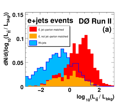
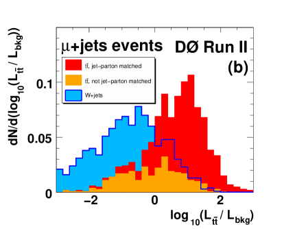
Abbildung 37: D0 Matrix Element analysis in the $\ell$$+$jets channel [39]: Distributions of $\log_{10}(L_{t\bar{t}}/L_{\rm bkg})$ for $t\bar{t}$ events with $m_{t}=175\,\,\mathrm{Ge\kern-1.00006ptV}$ (red and orange areas) and $W$$+$jets events (dark blue lines) for (a) $e$$+$jets events and (b) $\mu$$+$jets events. The $L_{t\bar{t}}$ values are calculated for the assumption $m_{t}=175\,\,\mathrm{Ge\kern-1.00006ptV}$. The distributions for signal and background events are normalized individually. Those $t\bar{t}$ events where all jets can be matched to partons are shown in red, while $t\bar{t}$ events that fail this requirement give rise to the orange distributions.

10.3 Fit Results

In this section, the fit results of the CDF template [67] and D0 Matrix Element [39] analyses in the $\ell$$+$jets channel are described. These measurements have been chosen in order to give one example for each of the two fitting techniques.

The reconstructed $m_{t}^{\rm reco}$ and $m_{jj}$ estimator distributions in data are shown in Figures 38 and 39, respectively, for the CDF template measurement. The parametrized template distributions corresponding to the fitted parameters are overlaid.

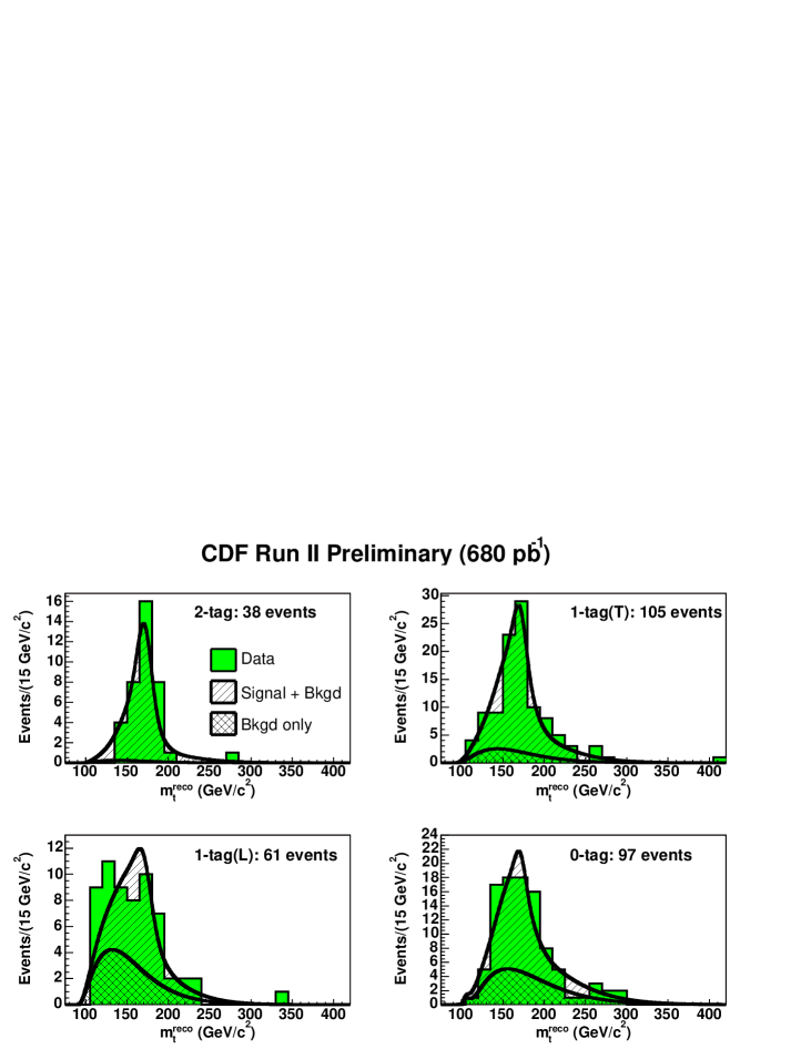
Abbildung 38: CDF lepton+jets template measurement [67]: Data $m_{t}^{\rm reco}$ distributions in the (a) 2-tag, (b) 1-tag(T), (c) 1-tag(L), and (d) 0-tag event categories, together with the parametrized template distributions for signal+background and background only that correspond to the fitted parameters.

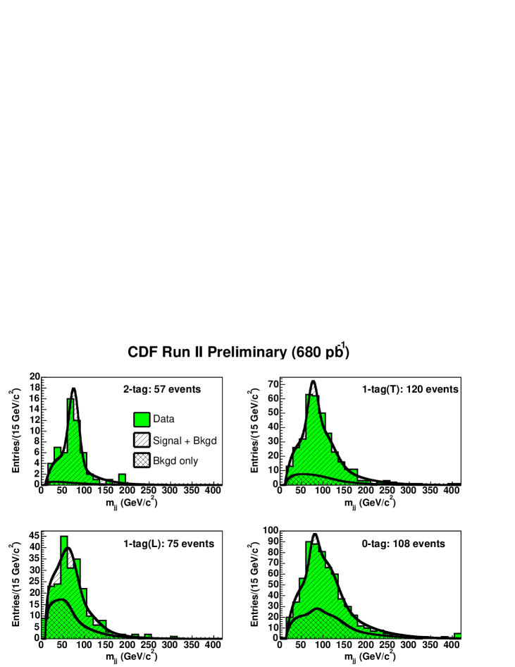
Abbildung 39: CDF lepton+jets template measurement [67]: Data $m_{jj}$ distributions in the (a) 2-tag, (b) 1-tag(T), (c) 1-tag(L), and (d) 0-tag event categories, together with the parametrized template distributions for signal+background and background only that correspond to the fitted parameters.

In the template measurement, the combined fit to the estimator distributions yields the likelihood as a function of assumed $m_{t}$ and $JES$ values. In the Matrix Element technique, this information is determined from the individual event likelihoods. These results, including the statistical uncertainties, are visualized in Figure 40 for the two measurements. Contours are shown corresponding to $\Delta\ln L=0.5$, $2.0$, $4.5$, and $8.0$ relative to the minimum $-\ln L$ value, where $L$ denotes the likelihood for the event sample. The calibrations for $m_{t}$ and $JES$ derived as discussed in the previous section are taken into account.

Abbildung 40: Results of the fits to determine the top quark mass and jet energy scale. (a) CDF template measurement in the $\ell$$+$jets channel [67]. (b) D0 Matrix Element measurement in the $\ell$$+$jets channel [39]. In both cases, the contours corresponding to $\Delta\ln L=0.5$, $2.0$, $4.5$, and $8.0$ relative to the minimum are shown. Note that in (a) the jet energy scale (vertical axis) is measured in units of the uncertainty $\sigma_{c}$ of the external calibration, while in (b) (horizontal axis) the multiplicative scale factor for jet energies is given.

The results quoted by the D0 collaboration are obtained from the projection of the likelihood onto the $m_{t}$ and $JES$ axes as described in Section 10.1.2. These projections are shown in Figure 41 together with the fitted curves. The central values and 68% confidence level intervals are also indicated.

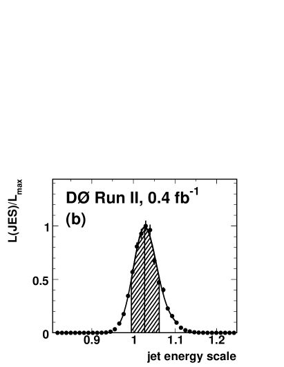
Abbildung 41: One-dimensional projections of the likelihood obtained in the D0 Matrix Element measurement in the $\ell$$+$jets channel shown in Figure 40(b) [39]. Plot (a) shows the likelihood as a function of assumed top quark mass. The correlation with the jet energy scale is taken into account. The fitted curve is shown, as well as the most likely value and the 68% confidence level region. The corresponding plot for the $JES$ parameter is shown in (b).

The comparison of the fitted uncertainties with the expectation from pseudo-experiments is discussed in the previous section. The statistical uncertainty includes the uncertainty from the absolute jet energy scale. The contribution of the absolute jet energy scale to the total statistical uncertainty can be estimated by repeating the fit with the $JES$ parameter fixed. It should however be noted that fitting for one overall factor does not cover the entire systematic uncertainty due to the jet energy scale, cf. Section 11.2.1.

11 Systematic Uncertainties

The previous section described how the central measurement value of the top quark mass and the associated statistical uncertainty are determined. To date, the world-average value for the top quark mass is already systematically limited. This section discusses the individual sources of systematic errors, describes the correlations among various measurements and how they are handled in the combination, and indicates where systematic uncertainties may be reduced in the future.

With the increasing size of the datasets collected at Run II of the Tevatron, the precision of the world-average value of the top quark mass has already become limited by systematic uncertainties. This is in spite of the fact that the measurement techniques have been improved during the past years. In particular, the determination of the jet energy scale from the same data that is used to measure the top quark mass has reduced the systematic uncertainty due to the detector calibration. Thus, the initial expectations for Run II of the Tevatron have already been surpassed. At the LHC, systematic effects will become even more dominant.

In this section, the different sources of systematic uncertainties are discussed together with the way they are typically evaluated. Systematic correlations between measurements or experiments, which will tend to reduce the beneficial effect of combining several measurements, are mentioned. Also indicated are ideas for future improvements, as well as limitations.

Systematic uncertainties can be broadly classified into three categories: modeling of the physics processes for $t\bar{t}$ production and background, modeling of the detector performance, and uncertainties in the measurement methods. The following discussion is ordered along the lines of this classification.

In Table 4 an overview of systematic uncertainties is given, quoting both the uncertainties on the world-average top quark mass [9] (which is only available in broad categories) and on one individual measurement [39].

Source of Uncertainty	World Average	D0, Lepton+Jets Channel
Statistical uncertainty	$\pm 1.2$	$\pm 2.5\enspace$
Physics modeling:	$\pm 1.0$
PDF uncertainty		$+0.16\leavevmode\nobreak\ -0.39$
ISR/FSR modeling		$\pm 0.46$
$b$ fragmentation		$\pm 0.56$
$b$/$c$ semileptonic decays		$\pm 0.05$
$W$$+$jets background modeling		$\pm 0.40$
QCD contamination		$\pm 0.29$
Detector modeling:	$\pm 1.4$
Absolute jet energy scale		$+3.2\leavevmode\nobreak\ -3.7$
$JES$ $p_{T}$ dependence		$\pm 0.19$
$b$ response (h/e)		$+0.63\leavevmode\nobreak\ -1.43$
Trigger		$+0.08\leavevmode\nobreak\ -0.13$
$b$ tagging		$\pm 0.24$
Noise, multiple interactions		—
Method:	$\pm 0.3$
Signal fraction		$\pm 0.15$
MC calibration		$\pm 0.48$
Total uncertainty	$\pm 2.1$	$+4.3\leavevmode\nobreak\ -4.9$

Tabelle 4: Summary of uncertainties on the top quark mass. All values are quoted in GeV. Uncertainties on the world-average value [9] are quoted in the second column. Only values corresponding to a broad classification of error sources are available for the world average. Some values from [9] have been combined to reflect the categories used here. The detector modeling uncertainty is dominated by that on the absolute value $JES$ of the jet energy scale. The right column shows uncertainties for the D0 Matrix Element measurement in the $\ell$$+$jets channel [39]. For asymmetric uncertainties the upper and lower errors are quoted separately. The uncertainty from the absolute $JES$ value has been listed together with the systematic uncertainties in the right column even though it is determined with in situ calibration and scales with statistics.

11.1 Physics Modeling

Many different processes can lead to the $t\bar{t}$ event candidates selected for a top quark mass measurement, and not all of them can be taken into account in the simulation. In addition, the description of the processes that are accounted for may still be subject to uncertainties. This type of uncertainties is discussed in this section, while effects not arising from a single hard interaction (multiple interactions) are treated in Section 11.2.

The top quark decay properties are well-known in the Standard Model, including the subsequent decay of the $W$ boson into partons, since these decays are governed by the weak interaction and the top quark does not hadronize. The top quark width as a function of its mass is known [3], and the branching fraction of the decay $t\to Wb$ is $100\%$ for practical purposes. Furthermore, the mass, width, and branching fractions of the $W$ are known precisely [3] and the associated uncertainties can be neglected.

In contrast, significant uncertainties do arise from the production of the $t\bar{t}$ pair (modeling of the parton distribution functions and of initial-state radiation) and the formation of final-state jets (final-state radiation, fragmentation, and hadronization modeling). Usually, the Monte Carlo simulation of $t\bar{t}$ events is based on the leading-order matrix element for the processes $q\bar{q}\to t\bar{t}$ and $gg\to t\bar{t}$. However, next-to-leading-order Monte Carlo simulation is already available [87]. The PDF parametrization and the modeling of initial- and final-state radiation have to be matched with the description of the hard-scattering process accordingly. The general description below remains however valid in both cases.

11.1.1 PDF Uncertainty

Parton distribution functions (PDFs) parametrize the probability to find a parton of a given flavor and momentum fraction inside the proton or antiproton, and thus the kinematic distributions of signal and background events depend on the PDFs. The Tevatron experiments have agreed on a common procedure to evaluate the top quark mass uncertainty related to PDF modeling, which is described for example in [39]. Typically, the simulated events used to calibrate the measurements (cf. Section 10.2) are based on a leading-order PDF set like CTEQ5L [22]. Systematic variations are however only provided for the PDF set CTEQ6M [27]. Therefore, the top quark mass is recomputed with a calibration based on the central CTEQ6M PDF set, and the differences between that value and the ones obtained with the systematic variations of the CTEQ6M PDF are added in quadrature and assigned as a systematic uncertainty. Note that the difference between top quark masses evaluated with the calibrations based on the CTEQ5L and central CTEQ6M PDF sets is not included in the uncertainty. The difference between the results obtained with the CTEQ5L and MRST leading-order PDF sets is taken as another uncertainty. Finally, the effect from using MRST PDF sets based on different assumed $\alpha_{s}$ values is determined. These three individual systematic uncertainties are summed in quadrature, the variation of CTEQ6M parameters yielding the dominant contribution.

For the determination of the world-average top quark mass, the resulting error is taken as $100\%$ correlated between individual measurements. The size of the uncertainty is given in Table 4 for the D0 measurement in the lepton+jets channel. The individual contributions are

CTEQ6M variations:	$+0.12$ $-0.38$ GeV,
difference MRST$-$CTEQ5L:	$\pm 0.09$ GeV,
variation of $\alpha_{s}$:	$+0.06$ $-0.03$ GeV.

Since this systematic error is correlated between all measurements, a common procedure for its evaluation like the one described above is important. Improvements of the above scheme are however still desirable and possible:

• The use of a leading-order matrix element together with a PDF set intended for processes in next-to-leading order is not consistent. The calibration of future measurements of the top quark mass should be based on next-to-leading-order Monte Carlo simulation using CTEQ6M (or updated PDF sets for which systematic variations are available), which would naturally resolve this inconsistency.

• Different top quark mass measurements may be more or less sensitive to variations of individual parameters describing the PDF set. For example, depending on kinematic event selection cuts, the relative importance of the gluon PDF may vary even considering only Tevatron analyses; this will become a more important issue when measurements at the LHC are included as well, where the $gg\to t\bar{t}$ process dominates. Consequently, the quadratic sum resulting from the variations of all PDF parameters should not be taken as 100% correlated between measurements, but top quark mass shifts should be quoted for each individual PDF parameter variation. This will then allow for a more refined computation of the uncertainty on the world average, potentially slightly reducing the overall systematic error due to PDF uncertainties. (Note that no extra systematic uncertainties will have to be evaluated, only a more refined report of individual variations is needed.)

• The comparison of top quark masses obtained with leading-order CTEQ and MRST PDF sets aims to quantify potential uncertainties arising from different PDF fitting procedures. However, these PDF sets are not based on exactly the same inputs, leading to additional differences that should already be covered by the variation of CTEQ parameters. Since the systematic error arising from the CTEQ/MRST comparison is small, this is currently not an important issue.

Currently, the systematic top quark mass error related to PDF uncertainties does not dominate the world average, cf. Table 4. Because it is correlated between individual measurements, it may become important in the future, but only if no further improvements on PDF uncertainties are assumed.

11.1.2 Initial- and Final-State Radiation

Radiation off the incoming and outgoing partons may affect the top quark mass measurement. Such radiation changes the kinematics of the $t\bar{t}$ decay products in the final state; for example, the transverse momentum of the $t\bar{t}$ system is not zero when initial-state radiation (isr) takes place. Final state radiation (fsr) changes the momenta of the $t\bar{t}$ decay products and thus affects the shapes of templates or the signal probability assigned to an event. Also, isr or fsr may lead to jets which can be misidentified as $t\bar{t}$ decay products.

Initial- and final-state radiation are governed by the same equations and are modeled in the shower evolution in the Monte Carlo simulation. (Interference between isr and fsr cannot be taken into account in this simulation, only when next-to-leading matrix elements are used.) The CDF experiment has shown how the details of the radiation process can be studied with Drell-Yan events [38, 57]. In Drell-Yan events only isr is present (photon radiation off charged leptons is assumed to be well-modeled, so only QCD radiation is considered here); it can lead to a non-zero transverse momentum $p_{T}$ of the dilepton system. The mean dilepton $p_{T}$ is shown to have a linear dependence on the logarithm of the dilepton invariant mass, which is reproduced by pythia simulation with standard parameter settings, cf. Figure 42. The study of Drell-Yan events also motivates two alternative pythia parameter sets leading to more or less isr and fsr activity, which are used to evaluate the systematic uncertainty on the top quark mass. The parameters changed are $\Lambda_{\rm QCD}$ and the scale factor $k$ to the transverse momentum scale for isr showering; settings of $\Lambda_{\rm QCD}=292\,\,\mathrm{Me\kern-1.00006ptV}$ and $k=0.5$ are used for the sample with increased isr activity, while $\Lambda_{\rm QCD}=73\,\,\mathrm{Me\kern-1.00006ptV}$ and $k=2.0$ are taken for the sample with less isr. The resulting mean dilepton $p_{T}$ values are also indicated in Figure 42.

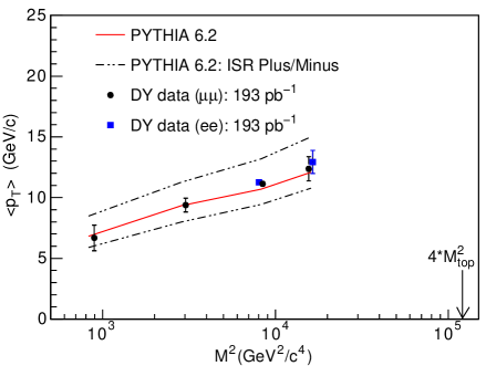
Abbildung 42: The average $p_{T}$ of the dilepton system in Drell-Yan events, which is a measure of the level of isr activity, as a function of the dilepton invariant mass squared (note the logarithmic horizontal scale) [38, 57]. The points with error bars indicate CDF measurements, while the solid and dashed lines show predictions by the pythia generator (standard parameter settings and variations for systematic error evaluation, respectively).

The approach followed by D0 in [39] is instead to vary directly the fraction of events with significant radiation. The calibration of the measurement is repeated based on events where a $t\bar{t}$ pair is produced together with an additional parton. Since the cross-section for $t\bar{t}$ production is 30% larger in next-to-leading order than in leading order, 30% of the observed difference between the top quark masses measured with the default and this alternative calibration is assigned as systematic uncertainty.

In the $\ell$$+$jets channel, the CDF experiment quotes a systematic uncertainty of 0.5 GeV for their template measurement [67], while the Matrix Element measurement is more sensitive to the modeling and finds a 1.0 GeV uncertainty [66] (adding isr and fsr uncertainties in quadrature). For the D0 Matrix Element measurement in the $\ell$$+$jets channel, a systematic error of 0.5 GeV has been evaluated [39] (see Table 4) using a different technique as described above. Similar uncertainties have been obtained in the dilepton [75, 76, 88] (0.4 GeV, 0.6 GeV, and 0.7 GeV, respectively) and all-jets channels [69] (0.7 GeV), where the values quoted are from the measurements using $1\,\,\rm fb^{-1}$ of data.

In the future, the uncertainty in isr and fsr modeling may become a dominant systematic error since it is correlated between all measurements. For consistency, it would therefore be highly desirable to arrive at an agreement between experiments on how to evaluate it, as is the case for the PDF error, see Section 11.1.1. In addition, more precise studies of isr and fsr should be carried out. The analysis of Drell-Yan events that the CDF experiment has published in [38, 57] can be repeated with much more data and thus extended to larger invariant dilepton masses, so that the extrapolation to $t\bar{t}$ events becomes smaller. This may allow to decrease the width of the error band shown in Figure 42. In addition, an examination of LEP/SLC results on hadronic $Z$ decays may yield independent experimental information on fsr. Finally, it may soon become worthwhile to optimize the measurement techniques not only in view of the statistical error, but to also keep systematic effects in mind. An idea developed for the LHC is to consider events in which the top and antitop quarks have large $p_{T}$, which means that their decay products are found in two separate event hemispheres; the mass of the top quark with the hadronic $W$ decay could then be reconstructed from the individual hadrons, making jet reconstruction superfluous and rendering the measurement mostly insensitive to final-state radiation [89]. But already the simultaneous $JES$ fit in the $\ell$$+$jets Matrix Element analyses at the Tevatron has proven to reduce the sensitivity of the result to radiation modeling [90], and an additional integration over the $t\bar{t}$ transverse momentum, as used in [74], may further reduce this uncertainty.

11.1.3 Fragmentation

Related to final-state radiation are the formation of jets in the final state and the spectra of hadrons within the jets. The fragmentation and hadronization of $b$-quark jets is particularly important: in dilepton events, only $b$-quark jets are expected (except for jets from isr or fsr), and in $\ell$$+$jets and all-jets events, in situ calibration of the jet energy scale can largely absorb the dependence on the modeling of light ($u$, $d$, $s$, $c$) quark jets. Simulations based on different fragmentation and hadronization models may predict different average energy fractions contained within the reconstructed jet; this leads to an uncertainty on the relation between jet and parton energies and thus on the measured top quark mass. In addition, $b$-quark fragmentation also affects the efficiency of $b$-jet identification: for a given $b$-quark energy, an increase of the average energy fraction $\langle x\rangle$ carried by the bottom hadron will lead to a higher probability to detect a well-separated secondary decay vertex even for low-energy $b$ quarks and will thus affect the kinematic distribution of the selected events.

Data from LEP and SLC on $Z\to b\bar{b}$ decays constrain $b$ fragmentation models and yield for example a precise determination of the mean energy fraction $\langle x_{b}\rangle$ of the weakly-decaying bottom hadron in $Z$ decays [1]. To extrapolate to $t\bar{t}$ decays, different fragmentation models that are consistent with $Z$ data are used to simulate $t\bar{t}$ events and the corresponding distribution in top quark decays (References [91] define $\langle x_{B}\rangle$ as the bottom hadron energy divided by the maximum possible $b$-quark energy). To evaluate the uncertainty on the top quark mass, the calibration of the measurement is determined using these different models, and the observed differences in the top quark mass are assigned as systematic error.

Uncertainties in the decay of bottom (and charm) hadrons can also play a role. In particular, jets containing a semileptonic decay of a heavy hadron will on average be reconstructed with a smaller energy due to the escaping neutrino. Thus the top quark mass depends on the rate and modeling of semileptonic heavy hadron decays. To assess uncertainties in the decay model, the semileptonic branching fractions of heavy hadrons in $b$-quark jets are varied within the bounds from measurements in $Z$ decays [1].

Like the other systematic errors related to physics modeling, the resulting uncertainties are correlated between measurements. The semileptonic branching fractions are known so precisely that the associated systematic error is negligible; however, the $b$-quark fragmentation uncertainty may become a dominating uncertainty in the future, see Table 4. As a first step, a common scheme for evaluating this uncertainty should be agreed on. This could be the definition of a set of fragmentation models and parameters (like the ones studied in [39]) on which the evaluation of uncertainties is based for each measurement. Such a common definition would not only lead to a consistent evaluation of uncertainties, but also allow for a correct determination of systematic correlations between individual measurements. As a next step, measurement techniques with reduced sensitivity to the details of $b$-quark fragmentation could be developed. The technique based on high-$p_{T}$ top quarks mentioned in Section 11.1.2, which does not rely on conventional jet finding, may serve as an example, but will need to be refined to optimize the overall uncertainty.

11.1.4 Top Quark Mass Definition

A top quark mass measurement based solely on invariant mass reconstruction from the momenta of the decay products corresponds to a measurement of the pole mass. All results available today are based mainly on properties of the $t\bar{t}$ decay products which in turn depend on the top quark (pole) mass; the current measurements can therefore be regarded as pole mass measurements to a good approximation. However, calculations of effects involving the top quark mass like the ones described in Sections 12.2.1 and 12.2.2 are typically not performed using the pole mass. The transformation into the $\overline{\rm MS}$ scheme is known to three loops and is e.g. given in [3]; such a transformation introduces an uncertainty when interpreting the top quark mass.

Measurements in the dilepton channel necessarily include other information as well since the kinematics of the $t\bar{t}$ system is underconstrained; also measurements in the $\ell$$+$jets and all-jets channels make use of additional information from the $t\bar{t}$ production process to a varying degree in order to reduce the statistical measurement uncertainty. It still remains to be studied to what extent this fact leads to an uncertainty in the interpretation of the measurement results.

In addition to the above, the pole mass itself is not defined to arbitrary accuracy for a colored particle like the top quark, and there is necessarily some additional color flow involved in the creation of the colorless final state measured in the detector. It has been shown in [18] that this introduces an intrinsic uncertainty of the order of $\Lambda_{\rm QCD}$ on the pole mass. The exact size of the uncertainty depends on the details of the measurement, and detailed studies of this effect are only starting.

11.1.5 Color-Reconnection Effects

Apart from the intrinsic uncertainty on the pole mass of a colored particle, color-reconnection effects between the final-state products may lead to additional effects. Corresponding studies for the measurement of the $W$ boson mass at LEP2 are described in [2]. The effect in $WW$ production at LEP2 is small compared to uncertainties on the top quark mass (a $35\,\,\mathrm{Me\kern-1.00006ptV}$ systematic error is quoted in the all-jets $WW$ final state) in the present and near future. The all-jets $WW$ final state may be considered similar to $\ell$$+$jets $t\bar{t}$ events; however, the kinematics are different; the colored beam remnants may well play an additional role in $t\bar{t}$ events at hadron colliders, and it is not clear how in situ calibration of the jet energy scale is affected. It is expected that the results of first studies of the size of color-reconnection effects will be published soon [92].

11.1.6 Bose-Einstein Correlations

The LEP experiments have determined the effects from Bose-Einstein correlations between particles in $WW$ events [2]. The resulting uncertainty on the top quark mass has not yet been studied, but it can be expected to be of the same order as that assigned to the $W$ mass measured in the all-jets $WW$ final state ($7\,\,\mathrm{Me\kern-1.00006ptV}$ [2]). Such an uncertainty would be negligible for the top quark mass.

11.1.7 Underlying Event

In principle, particles produced from the remnants of the colliding hadrons may contribute energy to the jets reconstructed in the detector. It is therefore necessary to measure the average contribution and subtract it from the jet energies. This is done as part of the jet energy calibration. The resulting uncertainty is small, as shown in Figure 14, and included in the jet energy scale uncertainty (even though it is in principle correlated between experiments).

11.1.8 Background Modeling

All physics uncertainties (except for the top quark mass definition) discussed in the previous sections affect the modeling of both signal and background events. In this section, additional uncertainties that are specific to the background model are discussed, separately for $\ell$$+$jets, dilepton, and all-jets events.

Lepton+Jets Channel:

The two main backgrounds in the $\ell$$+$jets channel are leptonically decaying $W$ bosons produced in association with jets ($W$$+$jets events) and multijet events containing a wrongly identified isolated lepton (QCD events). Both CDF (see e.g. [38, 66]) and D0 ([39]) find that the main uncertainty related to the modeling of $W$$+$jets background comes from a variation of the factorization scale $\mu_{F}^{2}$ used in the generation of these events. An additional contribution comes from the variation of the flavor composition of the jets in $W$$+$jets events [38, 66].

Both CDF and D0 base the estimate of QCD background on data. It is not straightforward to define a sample for this estimation that is kinematically unbiased and does not contain a sizeable $t\bar{t}$ component. Therefore, the QCD background estimate is replaced with $W$$+$jets events, and the resulting difference is conservatively quoted as systematic error.

The CDF values quoted for the uncertainty from modeling of $W$$+$jets and QCD events are 0.2 GeV [66] and 0.5 GeV [38], but cannot be compared directly to the D0 value of $0.4\oplus 0.3\;\,\mathrm{Ge\kern-1.00006ptV}=0.5\;\,\mathrm{Ge\kern-1.00006ptV}$ [39] (see Table 4) since CDF and D0 consider different factorization scales, and D0 does not vary the heavy flavor content in $W$$+$jets events.

Dilepton Channel:

The main backgrounds in the dilepton channel come from diboson ($WW$, $WZ$) or Drell-Yan production ($Z/\gamma^{*}\to e^{+}e^{-},\mu^{+}\mu^{-},\tau^{+}\tau^{-}$) in association with jets, and from events with a mis-identified electron (e.g., $W(\to\mu\nu)+3\,{\rm jets}$ with a jet faking an electron). To estimate the systematic uncertainty, the number of expected events from each source is varied independently within its error, and the resulting top quark mass shifts are added in quadrature [72, 73, 75, 76]. The systematic uncertainties assigned in individual top quark mass measurements vary between $\pm 0.3\,\,\mathrm{Ge\kern-1.00006ptV}$ and $\pm 1.0\,\,\mathrm{Ge\kern-1.00006ptV}$ (and even ${}^{+0.3}_{-1.9}\,\,\mathrm{Ge\kern-1.00006ptV}$). In addition, systematic variations of the background shapes yield another uncertainty of up to $\pm 1.0\,\,\mathrm{Ge\kern-1.00006ptV}$. Given the fact that the background contribution to the dilepton event samples is small while the statistical uncertainty is still large, it seems that some of these preliminary estimates are very conservative and that a much smaller uncertainty will be quoted in the future.

All-Jets Channel:

In this channel, the dominant background is from QCD multijet production. In the CDF analysis [69] the background is estimated from the data using a parametrization of the $b$-tagging efficiency. The overall normalization of this background estimate and the residual signal contribution are varied and each contribute a systematic error of $0.5\,\,\mathrm{Ge\kern-1.00006ptV}$ on the top quark mass. The accuracy of the background estimator is checked with signal depleted event samples, and no additional shape uncertainty is assigned.

The error on the world-average top quark mass that is due to background-specific uncertainties only amounts to $0.3\,\,\mathrm{Ge\kern-1.00006ptV}$ [9]. It will be possible to select $\ell$$+$jets and dilepton $t\bar{t}$ samples for top quark mass measurements with much smaller backgrounds at the LHC [89, 93] because of the larger $t\bar{t}$ cross section and better detector resolution, so that it can be expected that the uncertainty from background modeling will further diminish in the future.

11.2 Modeling of the Detector Response

For most individual measurements of the top quark mass, the dominant error is due to uncertainties in the detector response, most notably the jet energy measurement (see Table 4). Even though these errors are only correlated between measurements of one experiment, and despite the possibility of in situ $JES$ calibration, the absolute jet energy scale uncertainty still dominates the world average.

Because simulated events are used to calibrate the mass measurements, it is not the uncertainty on the absolute detector response that matters, but the uncertainty on the relative difference between the data and the simulation. Contributions can in principle arise from any aspect of the data related with the event selection and/or top quark mass reconstruction, ranging from uncertainties in the modeling of an energy dependence of event quality cuts, reconstruction or selection efficiencies, to the calibration of the reconstruction of the final-state leptons and jets.

11.2.1 Jet and Charged Lepton Energy Scales

In practice, by far the largest uncertainty arises from the uncertainty on the ratio of absolute jet energy scales in the data and simulation. Therefore, in situ calibration techniques are applied in the $\ell$$+$jets channel as described in Sections 7, 8, and 9. This means that the uncertainty on the absolute jet energy scales with the statistical error. The uncertainty obtained by D0 with $0.4\,\,\rm fb^{-1}$ is ${}^{+3.2}_{-3.7}\,\,\mathrm{Ge\kern-1.00006ptV}$ [39]; the CDF experiment quotes $2.5\,\,\mathrm{Ge\kern-1.00006ptV}$ using $0.68\,\,\rm fb^{-1}$ [67].

Without this technique, external measurements of the jet energy scale as described in Section 5.2 have to be used, and the uncertainty on the ratio between data and simulation propagated to the final result. The resulting systematic error is currently between $3$ and $5\,\,\mathrm{Ge\kern-1.00006ptV}$ in the $\ell$$+$jets [57], dilepton [72, 73, 75, 76, 88], and all-jets channels [58, 69] and is correlated between all measurements at the same experiment.

Even with in situ calibration, only one overall jet energy scale factor is determined. Any discrepancy between data and simulation other than such a global scale difference may lead to an additional uncertainty on the top quark mass, which is however much smaller than that arising from the overall absolute calibration. Uncertainties on residual $|\eta|$ and $p_{T}$ dependencies of the jet energy scale are taken from the external calibration and are typically estimated to be below $0.5\,\,\mathrm{Ge\kern-1.00006ptV}$, see for example References [39, 66] and Table 4.

The second-largest detector modeling uncertainty in the $\ell$$+$jets channel is the uncertainty on the double ratio between the jet energy scales for $b$-quark and light jets in the data and simulation. This error is due to differences between the calorimeter response to electromagnetic and hadronic showers and the uncertainty on the electromagnetic/hadronic energy ratio in $b$-quark jets. The CDF collaboration has evaluated it to be $\pm 0.6\,\,\mathrm{Ge\kern-1.00006ptV}$ [38, 66], and the D0 experiment has obtained ${}^{+0.6}_{-1.4}\,\,\mathrm{Ge\kern-1.00006ptV}$ [39].

In comparison with the energy scale for jets, the absolute energies of charged leptons are calibrated precisely using leptonic $Z$ decays. The uncertainty has been found to be negligible at D0 [90]; the CDF experiment quotes an uncertainty of $0.1\,\,\mathrm{Ge\kern-1.00006ptV}$ in the dilepton measurements [75, 76].

In the future, information from the overall jet energy scale calibration described in Section 5.2.1, which is not used in measurements with in situ calibration, can be introduced as an additional constraint to improve the world average. The uncertainty related to the $b$- to light-quark jet energy scale ratio may become a limiting systematic error in the mid-term future. Even though it is related to detector response, it is correlated between all measurements. The measurement of $Z\to b\bar{b}$ events has proven very difficult at the Tevatron, and event samples with a $b$ jet balanced by a photon or $Z$ decay are limited in statistics. Ideas for the an in situ calibration of this energy scale ratio would therefore be very helpful; otherwise radical techniques like a top quark mass measurement based on secondary vertex decay length information [68] or leptonic $J/\psi$ decays in top quark events [94] can be employed using the large-statistics samples at the LHC.

11.2.2 Event Selection

Uncertainties in the event selection efficiency, notably energy-dependent effects, can lead to systematic effects on the top quark mass. For example, the trigger efficiency is measured in the data using reference triggers, and the uncertainty on the dependence on charged lepton and jet energies is propagated to the top quark mass result. Similarly, the $b$-tagging efficiencies are determined from the data and varied within their uncertainties. Recent measurements in the $\ell$$+$jets channel quote systematic uncertainties of not more than a few hundred  $\mathrm{Me\kern-1.00006ptV}$ [38, 39]. Since the event selection efficiencies are calibrated using the data, it can be expected that the associated uncertainty will further diminish in the future.

11.2.3 Multiple Interactions

Bunch crossings with more than one hard interaction may lead to events where the $t\bar{t}$ decay products cannot be easily identified, or with additional energy contributions to the jets from the $t\bar{t}$ final state. As long as such events are modeled accurately, these effects can be taken into account in the calibration. However, uncertainties on the instantaneous luminosity and the properties of the additional hard interaction lead to a systematic uncertainty on the top quark mass. Recent CDF measurements quote a $0.05\,\,\mathrm{Ge\kern-1.00006ptV}$ [66] to $0.2\,\,\mathrm{Ge\kern-1.00006ptV}$ [75, 76, 88] uncertainty.

Overlay of calorimeter energy from subsequent bunch crossings was an issue at D0 Run I but is no longer significant due to a change in readout electronics [39].

11.3 Uncertainties Related to the Measurement Method

Since the calibration of a measurement method is based on simulated events, limited Monte Carlo statistics gives rise to a systematic uncertainty on the top quark mass. There may be other systematic errors inherent to a specific method. An example is the D0 Matrix Element measurement in the $\ell$$+$jets channel where the calibration depends slightly on the $t\bar{t}$ fraction in the selected event sample; the uncertainty on this fraction then leads to a systematic error on the top quark mass. Uncertainties of this type are normally uncorrelated between individual measurements, and are not dominant.

11.4 Summary

The precision of the world-average top quark mass is already limited by systematic errors [9]. Currently, the single largest uncertainty is due to the absolute jet energy scale. With in situ calibration using the hadronic $W$ mass, this error will be reduced with larger data sets. Until the startup of the LHC, physics modeling uncertainties (which are correlated between all measurements) will become dominant. In particular, work on the consistent evaluation (and reduction) of the uncertainties due to isr/fsr modeling, $b$-quark fragmentation, and the $b$/light jet energy scale ratio is very desirable in the near future.

12 Results, their Interpretation, and Future Prospects

This section gives an overview of the most recent measurements of the top quark mass and how they contribute to the world average. The current knowledge of the top quark mass is then set into perspective by discussing its implications for the Standard Model of particle physics, notably for consistency tests and indirect constraints on the mass of the Higgs boson. Finally, the prospects for future improvements of top quark mass measurements are outlined.

The Tevatron experiments have employed various methods to measure the top quark mass, as described in Sections 6-10. The most relevant individual measurements are combined by the Tevatron Electroweak Working Group, taking correlations into account as already outlined in Section 11. In Section 12.1 the individual measurement results are summarized, the combination procedure is described, and its current results are presented. Section 12.2 gives an interpretation of these results in the framework of the Standard Model and also discusses implications for the Minimal Supersymmetric Standard Model (MSSM). Finally, an overview of improvements to be expected with the startup of the LHC and a future linear $e^{+}e^{-}$ collider (ILC) is given in Section 12.3.

12.1 Measurement Results and Their Combination

A large number of measurements of the top quark mass has been performed to date at the Tevatron, using data in the $\ell$$+$jets, dilepton, and all-jets decay channels and applying a wide variety of measurement techniques [7, 8]. Table 5 summarizes the results.

Decay Channel	Measurement Technique (Section where described)	Exp./ Run	Int. Lumi. $[\,\rm fb^{-1}]$	Result [GeV]			Ref.	Weight
$\ell$$+$jets	T, mass reco. (7.1)	CDF II CDF II	$0.106$ $0.68\enspace$	$176.1$ $173.4$	$\enspace\pm 5.1$ $\enspace\pm 2.5$	$\enspace\pm 5.3$ $\enspace\pm 1.3$	[95] [67]	$\enspace-3.1\%\phantom{{}^{\dagger}}$
$\ell$$+$jets	T, multivariate	CDF II	$0.162$	$179.6$	$\enspace{}^{\phantom{0}+6.4}_{\phantom{0}-6.3}$	$\enspace\pm 6.8$	[96]
$\ell$$+$jets	T, decay length (7.2)	CDF II	$0.695$	$180.7$	$\enspace{}^{+15.5}_{-13.4}$	$\enspace\pm 8.6$	[68]	$\enspace+0.9\%^{\dagger}$
$\ell$$+$jets	ME, topological (8)	D0 II D0 II	$0.125$ $0.4\enspace\enspace$	$180.1$ $169.2$	$\enspace\pm 3.6$ $\enspace{}^{\phantom{0}+5.0}_{\phantom{0}-7.4}$	$\enspace\pm 3.9$ $\enspace{}^{\phantom{0}+1.5}_{\phantom{0}-1.4}$	[65] [39]	$\enspace+8.0\%\phantom{{}^{\dagger}}$
$\ell$$+$jets	ME, $b$ tagging (8)	CDF II D0 II	$0.94\enspace$ $0.4\enspace\enspace$	$170.9$ $170.3$	$\enspace\pm 2.2$ $\enspace{}^{\phantom{0}+4.1}_{\phantom{0}-4.5}$	$\enspace\pm 1.4$ $\enspace{}^{\phantom{0}+1.2}_{\phantom{0}-1.8}$	[66] [39]	$+61.7\%\phantom{{}^{\dagger}}$ $+18.9\%\phantom{{}^{\dagger}}$
$\ell$$+$jets	DL (8)	CDF II	$0.318$	$173.2$	$\enspace{}^{\phantom{0}+2.6}_{\phantom{0}-2.4}$	$\enspace\pm 3.2$	[57]
$\ell$$+$jets	ID (9)	D0 II	$0.4\enspace\enspace$	$173.7$	$\enspace\pm 4.4$	$\enspace{}^{\phantom{0}+2.1}_{\phantom{0}-2.0}$	[83]
dilepton	T, $p_{T}(\nu)$ (7.4)	CDF II CDF II D0 II	$0.109$ $0.359$ $0.835$	$167.4$ $170.7$ $171.6$	$\pm 10.3$ $\enspace{}^{\phantom{0}+6.9}_{\phantom{0}-6.5}$ $\enspace\pm 7.9$	$\enspace\pm 4.8$ $\enspace\pm 4.6$ $\enspace{}^{\phantom{0}+5.1}_{\phantom{0}-4.0}$	[97] [71] [72]	$\enspace-0.6\%\phantom{{}^{\dagger}}$
dilepton	T, $\phi(\nu)$ (7.4)	CDF II	$0.34\enspace$	$169.7$	$\enspace{}^{\phantom{0}+8.9}_{\phantom{0}-9.0}$	$\enspace\pm 4.0$	[71]
dilepton	T, $p_{z}(t\bar{t})$ (7.4)	CDF II	$1.02\enspace$	$168.1$	$\enspace{}^{\phantom{0}+5.6}_{\phantom{0}-5.5}$	$\enspace\pm 4.0$	[88]
dilepton	T, matrix weighting (7.4)	D0 II	$0.835$	$177.7$	$\enspace\pm 8.8$	$\enspace{}^{\phantom{0}+3.7}_{\phantom{0}-4.5}$	[73]	$-1.1\%^{\dagger}$
dilepton	T, $p_{T}(\nu)$ (7.4) and T, matrix weighting (7.4)	D0 II	$0.125$	$168.4$	$\pm 12.3$	$\enspace\pm 3.6$	[98]	$+0.6\%\phantom{{}^{\dagger}}$
dilepton	ME, topological (8)	CDF II	$1.03\enspace$	$164.5$	$\enspace\pm 3.9$	$\enspace\pm 3.9$	[75]	$\enspace+4.8\%\phantom{{}^{\dagger}}$
dilepton	ME, $b$ tagging (8)	CDF II	$0.955$	$167.3$	$\enspace\pm 4.6$	$\enspace\pm 3.8$	[76]
dilepton	DL (8)	CDF II	$0.34\enspace$	$166.6$	$\enspace{}^{\phantom{0}+7.3}_{\phantom{0}-6.7}$	$\enspace\pm 3.2$	[77]
all-jets	T (7.3)	CDF II CDF II	$0.109$ $1.02\enspace$	$186\phantom{.0}$ $174.0$	$\pm 10\phantom{.0}$ $\enspace\pm 2.2$	$\pm 12\phantom{.0}$ $\enspace\pm 4.8$	[99] [69]	$\enspace-0.3\%\phantom{{}^{\dagger}}$ $+10.3\%\phantom{{}^{\dagger}}$
all-jets	ID (9)	CDF II	$0.31\enspace$	$177.1$	$\enspace\pm 4.9$	$\enspace\pm 4.7$	[58]
$E\kern-6.00006pt/_{T}+{\rm jets}$	T	CDF II	$0.31\enspace$	$172.3$	$\enspace{}^{+10.8}_{\phantom{0}-9.6}$	$\pm 10.8$	[100]

Tabelle 5: Overview of top quark mass measurements. Analyses are grouped according to the $t\bar{t}$ decay channel listed in the leftmost column. The symbol “$E\kern-6.00006pt/_{T}+{\rm jets}$” denotes a selection based on $E\kern-6.00006pt/_{T}$ and jets only, yielding a sample enriched in events with a $W\to\tau\nu$ decay. The list is further ordered according to the analysis technique (T: template based; ME: Matrix Element; DL: Dynamical Likelihood; ID: Ideogram), given in the second column together with the section describing it. All recent CDF and D0 analyses of Run II data and those Run I measurements that are included in the world average [9] are listed. The experiment and integrated luminosity are given, and the top quark mass results are quoted with their statistical and systematic uncertainties. For measurements using in situ calibration, the uncertainty from the overall jet energy scale is included in the first quoted error as it will scale with statistics in future updates. The rightmost column lists the weight given to measurements in the world average value. For the measurements marked with a ^† sign, an earlier result is used in the combination, while the most recent value is given in the table.

No significant deviations are apparent between the top quark masses measured in individual decay channels, with different measurement techniques, by the two experiments, or at the two Tevatron center-of-mass energies of $1.8\,\,\mathrm{Te\kern-1.00006ptV}$ (Run I) or $1.96\,\,\mathrm{Te\kern-1.00006ptV}$ (Run II). However, many of the individual results are systematically and also statistically correlated. To quantify these statements, a consistent combination of results is performed by the Tevatron Electroweak Working Group [9] based on the best linear unbiased estimator (BLUE) [101, 102]. The procedure takes systematic correlations into account by treating individual systematic uncertainties as uncorrelated or 100% correlated between measurements as discussed in Section 11. More detailed studies are in general needed to evaluate the statistical correlation between measurements using the same dataset and decay channel. As an example, the statistical correlation between the top quark mass values determined at D0 in the topological Matrix Element analysis and the Ideogram measurement (which uses $b$ tagging) has been found to be only $+40\%$ [83, 90]. Since Tevatron Run II analyses are still evolving, such a study is not yet available in many cases. Therefore, a combination of Run I values and only the most precise Run II measurements in each channel is performed. The correlations between these measurements are close to zero unless a correlation arises via common jet energy scale uncertainties; in that case correlation coefficients are typically of the order of $30\%$, the largest being $56\%$ between the CDF Run I $\ell$$+$jets and Run II all-jets measurements.

The combination yields average top quark masses in the individual channels of

$$m_{t}({\text{$\ell$$+${\text{j}ets}}}) = 171.3\pm 2.2\,\,\mathrm{Ge\kern-1.00006ptV}\,,$$

$$m_{t}({\rm dilepton}) = 167.0\pm 4.3\,\,\mathrm{Ge\kern-1.00006ptV}\,,\ {\rm and}$$ (56)

$$m_{t}({\text{all-jets}}) = 173.4\pm 4.3\,\,\mathrm{Ge\kern-1.00006ptV}\,,$$

where the uncertainties include both statistical and systematic errors. The correlations ${\cal C}$ and resulting $\chi^{2}$ consistency values (for one degree of freedom) have been determined as

$$\begin{array}[]{rr@{\ }l}{\cal C}({\text{$\ell$$+${\text{j}ets}}},\ {\rm dilepton})=+37\%\,,&\chi^{2}({\text{$\ell$$+${\text{j}ets}}},\ {\rm dilepton})=1.2\,,\\ {\cal C}({\text{$\ell$$+${\text{j}ets}}},\ {\text{all-jets}})=+29\%\,,&\chi^{2}({\text{$\ell$$+${\text{j}ets}}},\ {\text{all-jets}})=0.24\,,&{\rm and}\\ {\cal C}({\rm dilepton},\ {\text{all-jets}})=+46\%\,,&\chi^{2}({\rm dilepton},\ {\text{all-jets}})=2.1\,.\end{array}$$ (57)

Since the values for all three channels are consistent with each other, one overall combined top quark mass value is computed. It is found to be

$$m_{t}=171.4\pm 2.1\,\,\mathrm{Ge\kern-1.00006ptV}\,.$$ (58)

The weights with which the individual top quark mass measurements contribute to this average are indicated in the last column of Table 5. Individual measurements may be assigned a negative weight in case of large correlations; as long as the weight is non-zero, the measurement still improves the average. This effect is explained very clearly and intuitively in [101]. The $\chi^{2}$ for the average is $10.6$ for $10$ degrees of freedom, and the largest single pull of any measurement that enters the combination is $1.8$, indicating good consistency of all $11$ measurements.

The $\ell$$+$jets, dilepton, and all-jets channels contribute with weights of $86.4\%$, $3.7\%$, and $10.0\%$ to the world average, respectively. These weights are indicative of the experimental situation at the Tevatron, with limited statistics in the dilepton and large backgrounds in the all-jets channel. With increasing data sets at Tevatron Run II, the relative importance of the dilepton channel may increase. Precise measurements of the top quark mass in the all-jets channel have only become possible after detailed studies of the background and its evaluation from the data. When in situ calibration techniques are applied in this channel, too, its weight may further increase.

12.2 Interpretation of the Top Quark Mass Measurement

As mentioned in Section 12.1, the top quark masses obtained in the $\ell$$+$jets, dilepton, and all-jets channels are consistent with each other. Moreover, the cross section for production of $t\bar{t}$ events at the Tevatron is consistent with the (Standard Model) expectation computed for the combined top quark mass value given in Equation (58). No average value of all Tevatron Run II measurements of the $t\bar{t}$ cross section exists yet; however, the CDF experiment has performed a combination of CDF measurements [103]. The D0 measurements can be found in [44, 106, 8]. Figure 43 shows the combined CDF result and the recent D0 measurement from Reference [44] together with the dependencies of the $t\bar{t}$ cross section measurements on the value of the top quark mass. Also shown are calculations of the $t\bar{t}$ cross section in next-to-leading order [13] as a function of the top quark mass. The measured cross sections agree well with the Standard Model prediction when assuming the world-average top quark mass value.

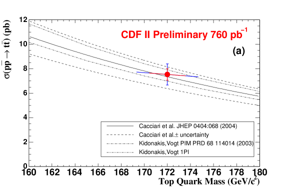
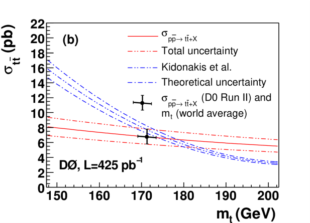
Abbildung 43: The average value of the $t\bar{t}$ production cross section in $p\bar{p}$ collisions at $\sqrt{s}=1.96\,\,\mathrm{Te\kern-1.00006ptV}$ as measured by the CDF experiment [103] is shown in (a). The vertical error bar indicates the $t\bar{t}$ cross section and its uncertainty evaluated at the CDF average value of the top quark mass. The dependence of the cross section measurement on the assumed top quark mass value is shown by the slope of the other error bar (its projection onto the horizontal axis corresponds to the uncertainty on the top quark mass using CDF measurements only). Also shown are NLO calculations of the Standard Model $t\bar{t}$ cross section, including threshold corrections from soft gluons [104, 105]. The uncertainty on these predictions is shown, too; it is dominated by the uncertainty on the gluon PDF. Consequently, no PDF uncertainty is included in the experimental result. Similarly, the result of a recent D0 measurement [44] is shown in (b) by the red lines, with the theoretical prediction from [104] overlaid. The combined information from the D0 $t\bar{t}$ cross section measurement and the world-average value of the top quark mass from is indicated by the crossed error bars. Note the different scales on the horizontal axes of the two plots.

Also other top quark measurements like the relative cross sections for the various decay channels or differential cross sections agree well with Standard Model predictions [7, 8]. Since there is no sign of effects beyond the Standard Model, it is appropriate to use the world-average top quark mass value in a consistency check of the Standard Model and, if consistency can be established, to extract information on Standard Model parameters. The interpretation within the Standard Model (SM) is discussed in Section 12.2.1. Analogously, the measurements can of course also be used to constrain the parameters of any other model that describes them. Particular attention has been devoted to supersymmetric models. The interpretation within the Minimal Supersymmetric Standard Model (MSSM) and the differences between MSSM and SM predictions are described in Section 12.2.2. While it is currently not yet possible to distinguish between the SM and MSSM based on indirect precision measurements, further improvements of these measurements may make this possible and thus provide information e.g. to help interpret potential future signals of new physics.

12.2.1 Interpretation within the Standard Model

An overall fit of Standard Model parameters is performed by the LEP Electroweak Working Group [2]. The general conclusion is that the Standard Model describes the measurements well and that there is no significant evidence for phenomena beyond the Standard Model.

(a)	(b)
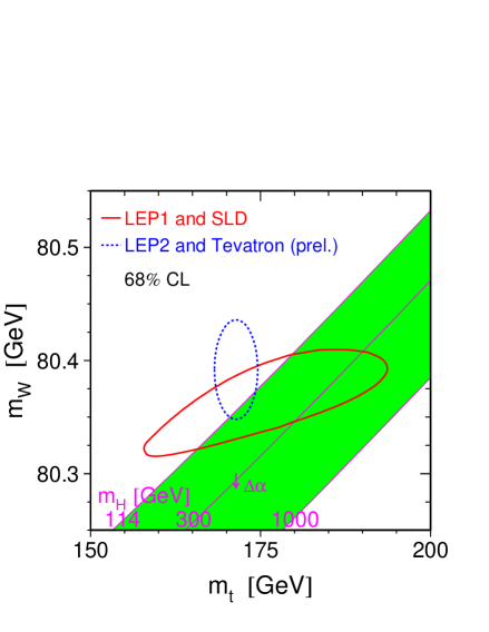
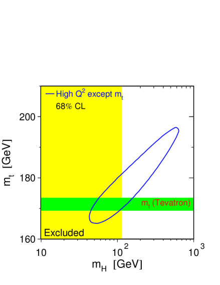
(c)	(d)

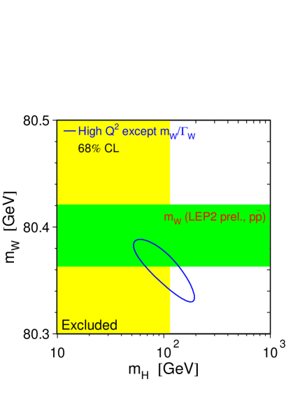
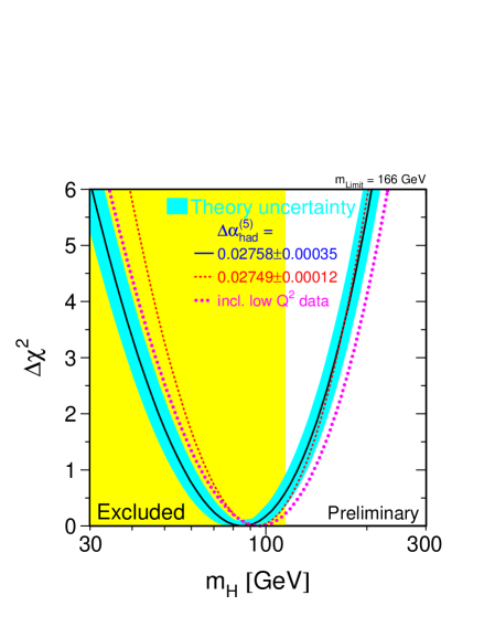
Abbildung 44: A comparison of direct measurements and indirect constraints within the Standard Model on the top and $W$ masses, as well as indirect constraints on the Standard Model Higgs mass [2]. (a) Direct measurements (blue dashed contour) of and indirect constraints (red solid contour) on $m_{t}$ and $m_{W}$ in the $m_{t}$-$m_{W}$ plane, together with the Standard Model prediction of the relation between $m_{t}$ and $m_{W}$ for various assumed Higgs masses. (b) Direct measurement of $m_{t}$ (green band) and indirect constraints on $m_{t}$ and $m_{H}$, excluding the direct $m_{t}$ measurement (blue contour). (c) Direct measurement of $m_{W}$ (green band) and indirect constraints on $m_{W}$ and $m_{H}$, excluding the direct $m_{W}$ measurement (blue contour). (d) Indirect constraint on $m_{H}$: $\Delta\chi^{2}$ with respect to the best fit as a function of assumed Standard Model Higgs boson mass. The light blue band indicates the uncertainty from higher-order corrections not included in the calculation. Also shown are fits including the NuTeV $m_{W}$ result (pink dotted curve) or based on a value of $\alpha(m_{Z})$ obtained with additional theoretical input (red dashed curve). In (b), (c), and (d) the yellow area shows the region of Standard Model Higgs masses excluded by direct searches.

Using the Standard Model relations, it is possible to infer information even on those parameters that have not (yet) been directly measured. Of particular interest is the constraint on the mass of the Higgs boson. As outlined in Section 2, within the Standard Model the mass of the $W$ boson depends quadratically on the top quark mass and logarithmically on the mass of the Higgs boson. This dependence is visualized in Figure 44. Figure 44(a) shows the agreement between direct measurements of the $W$ and top quark masses from LEP2 and the Tevatron, shown in blue, and indirect constraints that are valid within the Standard Model (red contour). Also shown is the Standard Model relation between $m_{W}$ and $m_{t}$ for various assumed values of the Higgs mass; the green band covers the range $114\,\,\mathrm{Ge\kern-1.00006ptV}<m_{H}<1000\,\,\mathrm{Ge\kern-1.00006ptV}$. The lower value of $m_{H}=114\,\,\mathrm{Ge\kern-1.00006ptV}$ corresponds to the direct exclusion limit from LEP searches.

Figure 44(b) shows how the top quark mass measurement contributes to the indirect constraint on the Higgs mass. In the $m_{H}$-$m_{t}$ plane, the blue contour depicts the information on these two parameters obtained from the Standard Model fit, where the direct $m_{t}$ measurement is not used as input. The projection of the blue contour onto the vertical axis thus corresponds to the indirect constraint on the top quark mass within the Standard Model of $m_{t}=178\,^{+12}_{\phantom{0}-9}\,\,\mathrm{Ge\kern-1.00006ptV}$ (note that a projection of the 68% C.L. contour from two dimensions to one does not correspond to one-dimensional 68% confidence limits). The green band corresponds to the direct top quark mass measurement, which is in good agreement with the indirect prediction. The band visualizes how this information, given the $W$ mass and other measurements, excludes large values of the Higgs mass within the Standard Model. Further improvements of the precision of the top quark mass measurement will improve the indirect constraint on the Higgs mass, but are unlikely to push this constraint into the region of mass values that has already been excluded at LEP, shown in yellow.

Similarly, the information on the Higgs mass obtained from the $W$ mass measurement is shown in Figure 44(c). The direct measurements of the $W$ mass, shown as the green band, are in agreement with the blue contour showing the indirect constraints. The contour from all measurements but the $W$ mass does not extend to high $m_{H}$ values in this plot since the top quark mass information is already included. With a significant improvement of the $W$ mass uncertainty the region of Standard Model self-consistency might be significantly reduced even before direct Higgs searches become sensitive beyond the current limit.

All indirect information on the Higgs boson mass is summarized in Figure 44(d), where the black curve shows the $\Delta\chi^{2}$ within the Standard Model as a function of assumed Higgs mass relative to the minimum value. The light blue band around it shows an estimate of the uncertainty from higher-order corrections that were not included in the calculation. Taking the information from this curve and including these theoretical uncertainties, the one-sided 95% C.L. upper limit on the Standard Model Higgs mass is $166\,\,\mathrm{Ge\kern-1.00006ptV}$. When the lower limit from direct searches is included, the upper limit shifts to $199\,\,\mathrm{Ge\kern-1.00006ptV}$.

In summary, the Standard Model yields a good description of experimental data; for example the top quark mass measurement is in good agreement with indirect constraints valid within the Standard Model. The top quark mass measurement is an important ingredient to fits in which indirect information on the mass of the Standard Model Higgs boson can be obtained. With the precision of the top quark mass value achieved with the techniques described in this report it is possible to place stringent upper bounds on the mass of the Higgs boson within the Standard Model.

12.2.2 Interpretation within the Minimal Supersymmetric Standard Model

Even though there is no compelling experimental evidence of physics effects beyond the Standard Model from collider experiments, it is instructive to interpret precision electroweak measurements also in extended models. As the top quark contributes via loop diagrams to the predictions for electroweak parameters, it is mandatory to know these contributions (and therefore the top quark mass) precisely to pin down any potential effects from additional, yet unknown, particles. In particular, a detailed study has been performed that compares the predictions of the Minimum Supersymmetric Standard Model (MSSM) [107] with those of the Standard Model (SM) in view of the precision measurements of the top quark and $W$ boson masses [108]. This study is summarized here.

After calculating contributions from loop diagrams involving supersymmetric particles, it is possible to compare the predictions of the SM and MSSM with each other and with the experimental data, as shown in Figure 45. The two model predictions lie within bands in the $m_{t}$-$m_{W}$ plane, with only a narrow overlap region. Apart from the fact that the red and blue regions correspond to a variation of the Standard Model Higgs mass between $114\,\,\mathrm{Ge\kern-1.00006ptV}$ and only $400\,\,\mathrm{Ge\kern-1.00006ptV}$, the information is equivalent to the predictions shown in Figure 44(a) where the upper value of the Higgs mass is set to $1000\,\,\mathrm{Ge\kern-1.00006ptV}$ (and the axes are scaled differently). The green and blue areas indicate the allowed region for the MSSM (in the region above the green area, at least one of the mass ratios $m_{{\tilde{t}}_{2}}/m_{{\tilde{t}}_{1}}$ and $m_{{\tilde{b}}_{2}}/m_{{\tilde{b}}_{1}}$ is larger than $2.5$, where in both cases the lighter mass state is denoted by the index 1). The MSSM allowed region was obtained by varying supersymmetry parameters independently from each other. In the Standard Model, the blue area which is allowed in both models corresponds to the case of a light Higgs boson within the range allowed in the MSSM, while in the MSSM, it corresponds to the case where all superparticles are so heavy that the theory becomes effectively equivalent to the Standard Model. The current direct measurements of the top quark and $W$ boson masses are shown by the blue ellipse. The black and red contours indicate rough estimates of the precision that can be achieved at the LHC and a future linear $e^{+}e^{-}$ collider (ILC), respectively (for the LHC, uncertainties on $m_{t}$ and $m_{W}$ of $1\,\,\mathrm{Ge\kern-1.00006ptV}$ and $15\,\,\mathrm{Me\kern-1.00006ptV}$ have been taken, respectively, while values of $0.1\,\,\mathrm{Ge\kern-1.00006ptV}$ and $7\,\,\mathrm{Me\kern-1.00006ptV}$ have been assumed for the ILC). The current central measurement values have been used to place these contours.

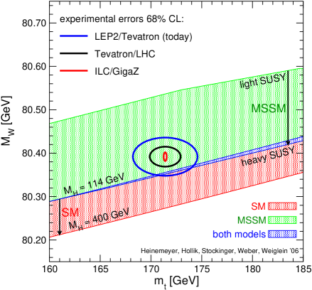
Abbildung 45: Comparison of predictions of the SM and MSSM with current and potential future direct measurements of $m_{t}$ and $m_{W}$. The figure is from [108] and has been prepared including calculations described in [109]. The area allowed in the SM corresponds to Higgs masses within the range $114\,\,\mathrm{Ge\kern-1.00006ptV}<m_{H}<400\,\,\mathrm{Ge\kern-1.00006ptV}$, while the MSSM region has been obtained in a parameter scan. The blue ellipse shows the current direct measurements, while the sizes of the black and red contours indicate potential future improvements of the uncertainties with data from the LHC and a future linear $e^{+}e^{-}$ collider, respectively (the central values for these contours are arbitrary).

Even though the central measurement values of $m_{t}$ and $m_{W}$ are not within the SM allowed region, based on the current data it is not possible to distinguish between the SM and MSSM. Nevertheless, it is evident that with increasing precision on $m_{t}$ and $m_{W}$, a comparison with model predictions may provide important constraints on the model parameters — or provide a cross-check of models to help decide which one is correct should physics effects beyond the Standard Model be discovered in the future.

Similar to the consistency check performed within the SM described in Section 12.2.1, it is possible to evaluate for models beyond the Standard Model which sets of parameter values are most likely. Such an analysis has for example been carried out in [110] for various constrained versions of the MSSM. The results tend to favor a relatively low MSSM scale, which would make the discovery of light supersymmetric particles possible at the LHC or even the Tevatron; an actual determination of parameter values of the MSSM can however not be performed with the current data.

12.3 Potential for Improved Top Quark Mass Measurements

Given the interpretation of the top quark mass measurement outlined in Section 12.2 above, it is clear that a further improvement of the experimental precision is desirable. The uncertainty on the current world average discussed in Section 12.1 is already dominated by systematic uncertainties. In the future, the focus will therefore have to shift from an optimization of the statistical uncertainty to a detailed study of the systematics listed in Section 11. In this quest, larger event samples will still help in two ways: First, some of the systematic errors are expected to improve with increasing sample sizes, and second, large event samples will allow to select small subsamples which are less prone to systematics than the rest.

In the following, the evolving situation at the Tevatron experiments is discussed first. Second, the prospects for measuring the top quark mass at the LHC are described. Finally, an outline of the potential for top quark mass measurements at a future linear $e^{+}e^{-}$ collider (ILC) is given.

12.3.1 Future Top Quark Mass Measurements at the Tevatron

With the Run IIa dataset not even fully analyzed, the Tevatron experiments have already surpassed the expectation that a combined top quark mass uncertainty of $2$-$3\,\,\mathrm{Ge\kern-1.00006ptV}$ would be possible with the full Run II dataset. This shows how important the newly developed techniques (Matrix Element method, in situ calibration) are, and how delicate it is to extrapolate from the current situation into the future. An extrapolation from the current combined result is particularly difficult as the world average combines different types of measurements based on data sets corresponding to different integrated luminosities. A general picture can however still be obtained from an analysis of how various measurements contribute to the current world average and of how the individual uncertainties of the most sensitive measurements will evolve.

From Table 5 it is obvious that the Run II measurements in the $\ell$$+$jets channel carry by far the largest weight (the two measurements that exploit full event reconstruction have a combined weight of $80.6\%$). The statistical sensitivities of the CDF [66] and D0 [39] Matrix Element measurements in the $\ell$$+$jets channel are quite similar; the difference in uncertainties comes from the difference in the size of the data sets analyzed so far and also from the fact that the observed D0 error is slightly larger than expected from simulations. Also, the systematic uncertainties are similar. Figure 46 shows how the uncertainties of the D0 measurement will evolve with statistics if the analysis is unchanged. All errors are assumed to remain constant except the statistical and $JES$ uncertainties which will be reduced with larger statistics. At the end of Run II, signal modeling and the $b$-jet energy scale will give rise to the limiting uncertainties. To estimate the reach of a combination of CDF and D0 analyses it is a good approximation to read off the diagram at the sum of integrated luminosities analyzed: The signal modeling uncertainties are fully correlated, and even the error due to the $b$-jet energy scale will be partly correlated as it is a combination of calorimeter response ($e/h$) and hadronization uncertainties.

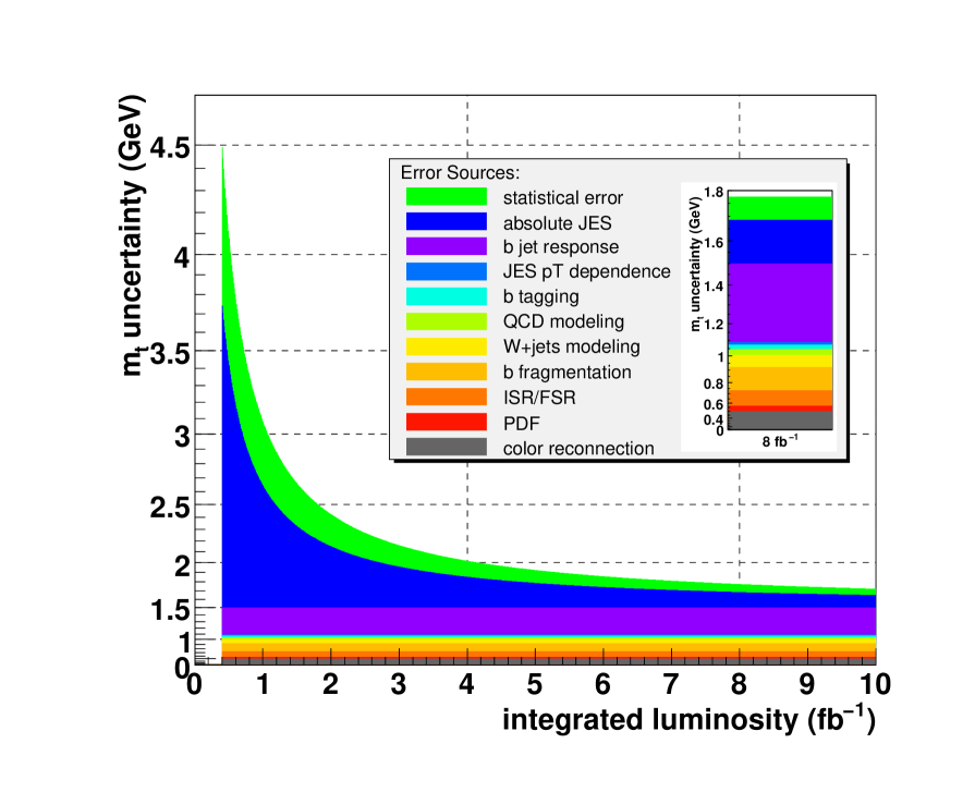
Abbildung 46: The composition of the uncertainty in the D0 Matrix Element measurement in the $\ell$$+$jets channel [39], which is based on an integrated luminosity of $0.4\,\,\rm fb^{-1}$, and the expected evolution of the uncertainty with integrated luminosity when the measurement technique is kept unchanged. An uncertainty of $0.5\,\,\mathrm{Ge\kern-1.00006ptV}$ to cover color reconnection effects, which have been shown in [18] to give rise to an effect of the order of $\Lambda_{\rm QCD}$, has conservatively been added (grey band), while the errors from semileptonic $b$- or $c$-hadron decays and from trigger efficiencies are negligible and have been omitted. The color code for the individual error contributions is explained in the figure. The widths of the colored bands indicate the individual squared uncertainties; the vertical axis is therefore non-linear and accounts for their quadratic addition. The two vertical dashed lines indicate the range of expectations for the integrated luminosity delivered to each Tevatron experiment by the end of Run II. The inset shows the expected uncertainties if the method is applied unchanged to an $8\,\,\rm fb^{-1}$ dataset. The figure is only intended to visualize the relative importance of various sources of uncertainty; it cannot provide accurate predictions for future measurements of the top quark mass.

While it is not justified to make more precise extrapolations into the future, the above indicates the areas where improvements are most needed. On the one hand, it will become important to develop measurement strategies that are less sensitive to the $b$-jet energy scale. An extreme example is the measurement based on the secondary vertex decay length [68]. One could also envisage for example a measurement based on the Matrix Element method which minimizes the combined statistical and systematic error by artificially worsening the $b$-jet energy resolution used in the probability computation, or which is extended to determine a $b$-jet energy response factor. On the other hand, it will be possible to repeat the studies of the $Z$ $p_{T}$ spectrum described in Section 11.1.2 with much larger samples, extend the invariant mass range, and obtain a more precise extrapolation to $t\bar{t}$ events. Dilepton measurements will be less affected by uncertainties on final-state radiation than those in the other channels. Currently, the dilepton channel contributes less than $5\%$ to the world average, which is mainly because no in situ calibration of the jet energy scale is used here. It would be very worthwhile to check if this is possible, as it would yield information on the $b$-jet energy scale. Even without in situ calibration, the CDF measurement in the all-jets channel [69] contributes to the world average with a weight of $10\%$. While events in this channel are well constrained kinematically, it remains to be seen if uncertainties due to hadronization and color reconnection can be kept under control.

In summary, it appears feasible that the total uncertainty on the top quark mass will be reduced from the current value of $2.1\,\,\mathrm{Ge\kern-1.00006ptV}$ to about $1.5\,\,\mathrm{Ge\kern-1.00006ptV}$ by the end of Tevatron Run II. The actual precision reachable will depend more on further innovative ideas on the treatment of systematics than on the exact integrated luminosity delivered.

12.3.2 Future Top Quark Mass Measurements at the LHC

The Tevatron measurements of the top quark mass have only been possible with a very good understanding of the detectors. After the startup of the LHC, it will still take some time until the LHC experiments will be able to improve the combined Tevatron result significantly. On the other hand, the physics of $t\bar{t}$ production will be well-understood from the Tevatron, and large samples will be selected, which can be used for the commissioning and calibration of the detectors – most notably, to determine the absolute jet energy scale and the $b$-jet identification efficiency.

Consequently, studies for the LHC experiments focus on two aspects: Detector commissioning with $t\bar{t}$ events [111, 112] and innovative measurements with reduced top quark mass systematics that are not feasible with Tevatron statistics [89, 93, 94]. Surely, top quark mass measurements will become a field of precision studies of systematic effects, but it is difficult to say today exactly what precision will finally be reached at the LHC for the top quark pole mass, as that depends on techniques that are only being developed now and will be developed further when the data is being taken.

An interesting proposal has been made in [113] to identify double-diffractive $t\bar{t}$ events at the LHC. In these events, the $t\bar{t}$ center-of-mass energy could be measured from the reconstructed protons, and a measurement of the $t\bar{t}$ cross section as a function of this center-of-mass energy would lead to a determination of the top quark mass. This technique would be complementary to measurements of the top quark pole mass from the properties of the decay products, and would rather be similar to a $t\bar{t}$ threshold scan at an $e^{+}e^{-}$ collider, which is outlined in the following section. If the cross section and integrated luminosity are large enough and the experimental challenges are solved, this measurement technique might be a way to overcome the principal theoretical limitations of top quark pole mass measurements at a hadron collider.

12.3.3 Future Top Quark Mass Measurements at the ILC

When a top-antitop cross section measurement is compared to predictions, this comparison yields a measurement of the parameter “top quark mass” that was used in the calculation of the prediction. Because of its large width, the top quark does not hadronize, but the $e^{+}e^{-}\to t\bar{t}$ production cross section still rises steeply at the energy corresponding to a 1S resonance, and the top quark mass can be determined from the energy where this rise is observed. (At larger energies, the cross section varies much less rapidly with center-of-mass energy, leading to a larger uncertainty when interpreted in terms of the top quark mass.) Suitable definitions of the top quark mass for such calculations (so-called “threshold mass” definitions) are discussed in [21].

At an $e^{+}e^{-}$ collider, $t\bar{t}$ events will have a striking experimental signature and can be selected with very low backgrounds. This means that the event selection can be kept simple enough so that it does not (or only very marginally, thus not introducing large uncertainties) depend on the exact properties of the top quark decay products — which would otherwise result in a measurement of the top quark pole mass, as discussed before in Section 2.1. In addition to the clean signature by which $t\bar{t}$ events can be selected, another prerequisite for this type of measurement is that the initial state is well-known. This is the case for an $e^{+}e^{-}$ collider (where only initial-state photon radiation has to be taken into account), but not for a hadron collider where the partons that initiate the hard interaction are only a part of the colliding hadrons.

References [114, 115] quote experimental uncertainties of $20$-$30\,\,\mathrm{Me\kern-1.00006ptV}$ on the 1S top quark mass. An uncertainty of $\Delta\alpha_{s}(m_{Z})=0.001$ corresponds to an uncertainty of $70\,\,\mathrm{Me\kern-1.00006ptV}$ in the conversion of the threshold mass to the $\overline{\rm MS}$ scheme [116], leading to an overall uncertainty on the $\overline{\rm MS}$ top quark mass of less than $100\,\,\mathrm{Me\kern-1.00006ptV}$.

In addition to the threshold scan, measurements of the top quark pole mass will of course also be possible at the ILC above the $t\bar{t}$ threshold; while the statistical and experimental systematic uncertainties may be small, the interpretation of such measurements will be limited by an additional uncertainty of order $\Lambda_{\rm QCD}$ as discussed before. Thus complex analysis techniques like the Matrix Element method will no longer be needed for the measurement of the top quark mass for which they were originally developed (but this does not invalidate them as a means of minimizing the statistical uncertainty in any other measurement based on few events whose kinematic properties are well-understood).

The possibility to determine the top quark mass via a threshold scan at the ILC corresponds to an order of magnitude improvement of the current uncertainty that will to current knowledge not be possible via explicit mass reconstruction from the decay products. The resulting constraints on the Standard Model or models beyond it will be very precise, as shown in Figure 45, and since the parametric uncertainties in the model predictions resulting from the top quark mass will be much smaller than today, stringent consistency tests of the models will be possible, as outlined for example in [117].

13 Summary and Conclusions

A measurement of the top quark mass is interesting per se because the top quark is by far the heaviest known elementary fermion. It is interesting also because the top quark mass is needed as an input parameter to calculations of electroweak precision variables – measurements of which can then be used to perform consistency tests of models or to obtain indirect information on as yet unmeasured parameters like the Higgs boson mass.

To date, top quarks can only be produced at the Fermilab Tevatron collider. The physics of top-antitop pair production and the resulting event topologies have been outlined. The reconstruction of the events has been described, it has been discussed how an accurate calibration of the detectors is indispensable for the measurement of the top quark mass, and the calibration procedures applied at the Tevatron experiments have been introduced. The determination of the absolute calorimeter energy scale is particularly challenging but also of particular importance for the measurement of the top quark mass.

Since the discovery of the top quark at Tevatron Run I, our understanding of $t\bar{t}$ production at hadron colliders has matured, much more integrated luminosity has been accumulated, and sophisticated techniques to measure the top quark mass have been developed that have led to an unanticipatedly large reduction of the uncertainty. These experimental techniques have been described in detail. On the one hand, this allows the reader to understand the details of the measurements of the top quark mass. On the other hand, this report is also intended as a reference for the methods, which can be used in the future for other measurements of similar experimental nature.

The current world-average value of the top quark mass is already dominated by systematic uncertainties. Their various sources have been discussed to identify the current limitations and to point out possible future improvements.

The interpretation of our current knowledge of the top quark mass within the Standard Model of particle physics has been presented. Current results of precision electroweak measurements are in striking agreement with Standard Model predictions, and thus the top quark mass can serve as an input to calculations with which constraints on the mass of the Standard Model Higgs boson can be placed. A similar interpretation can also be performed within extended models, and an analysis in the Minimal Supersymmetric Standard Model has been shown. Within the Standard Model, a light Higgs boson is clearly favored, and the data is also consistent with predictions within the Minimal Supersymmetric Standard Model.

Finally, the prospects for future measurements at the LHC and a linear $e^{+}e^{-}$ collider have been outlined. Many studies have been performed of how to measure the top quark mass based on the reconstruction of the final state in $t\bar{t}$ events at the LHC. At the LHC much larger event samples will be available than at the Tevatron. The LHC experiments will thus be able to improve the Tevatron results: Given the large event samples, systematic uncertainties related to detector calibration can be reduced, and other uncertainties may be improved by a careful selection of special subsamples of $t\bar{t}$ events for the mass measurement. Measurements of the top quark pole mass will however always be limited by an intrinsic uncertainty of $\Lambda_{\rm QCD}$. This uncertainty can be overcome in a threshold scan by comparing the measured $t\bar{t}$ production cross section as a function of the $t\bar{t}$ center-of-mass energy with predictions calculated as a function of the top quark mass (where calculations are not done in terms of the pole mass). This measurement technique, applied at a future $e^{+}e^{-}$ collider, will allow for an order of magnitude improvement of the uncertainty on the top quark mass measurement.

Measurements of the top quark mass have already become so precise that interesting constraints can be placed on the Standard Model. It is foreseeable how the precision will further improve in the future. The measurement of the top quark mass will remain an important input for stringent consistency checks of the Standard Model or of models describing potential new discoveries.