TUM-HEP 753/10

Stringy surprises

Michael Ratz

Physik-Department T30, Technische Universität München,
James-Franck-Straße, 85748 Garching, Germany

There are many conceivable possibilities of embedding the MSSM in string theory. These proceedings describe an approach which is based on grand unification in higher dimensions. This allows one to obtain global string-derived models with the exact MSSM spectrum and built-in gauge coupling unification. It turns out that these models exhibit various appealing features such as (i) see-saw suppressed neutrino masses, (ii) an order one top Yukawa coupling and potentially realistic flavor structures, (iii) non-Abelian discrete flavor symmetries relaxing the supersymmetric flavor problem, (iv) a hidden sector whose scale of strong dynamics is consistent with TeV-scale soft masses, and (v) a solution to the $\mu$-problem. The crucial and unexpected property of these features is that they are not put in by hand nor explicitly searched for but happen to occur automatically, and might thus be viewed as “stringy surprises”.

1 Goals of string model building

The standard model (SM) of elementary particle physics is remarkably successful in describing experiments. There are three main reasons for going beyond the SM:

1. observational: neither the observed cold dark matter nor the baryon asymmetry can be explained in the SM;

2. conceptual: the SM is based on quantum field theory, in which, however, it appears difficult to incorporate gravity;

3. aesthetical: the structure and the parameters of the SM ask for a simple, arguably more fundamental explanation.

Solid observations contradicting the SM so far are mostly astrophysical and/or cosmological. There are many ways to extend the SM such as to explain these observations; perhaps even too many. One might therefore argue that one should search for theoretical guidelines that, in a way, reduce the arbitrariness in model building. In these proceedings, the guideline will be the requirement that the extension of the SM should be embedded into string theory, which is believed to unify quantum gauge theory with gravitation. This choice is motivated by the above reasons ➁ ‣ 1 and ➂ ‣ 1, and sort of ignores the most concrete arguments ➀ ‣ 1 for going beyond the SM. This approach builds on the observation that the gauge couplings appear to meet in the minimal supersymmetric extension of the SM, the MSSM, at the scale

$$M_{\mathrm{GUT}}~{}=~{}\text{few}\cdot 10^{16}\,\mathrm{GeV}\;,$$ (1)

and that the four-dimensional Planck scale $M_{\mathrm{P}}$ is numerically not too far from $M_{\mathrm{GUT}}$. Explanations of the smallness of the neutrino masses often rely on a similarly high scale. Even more, the fact that one generation of SM matter fits into the $\boldsymbol{16}$-plet of $\mathrm{SO}(10)$ is interpreted as strong evidence for unification along the exceptional chain [1]

$$\mathrm{E}_{3}=G_{\mathrm{SM}}~{}\subset~{}\mathrm{E}_{4}=\mathrm{SU}(5)~{}\subset~{}\mathrm{E}_{5}=\mathrm{SO}(10)~{}\subset~{}\mathrm{E}_{6}~{}\subset~{}\mathrm{E}_{7}~{}\subset~{}\mathrm{E}_{8}\;,$$ (2)

which is beautifully realized in the heterotic string  [2, 3] (cf. the discussion in [4]). Here $G_{\mathrm{SM}}$ denotes the SM gauge group,

$$G_{\mathrm{SM}}~{}=~{}\mathrm{SU}(3)_{C}\times\mathrm{SU}(2)_{\mathrm{L}}\times\mathrm{U}(1)_{Y}\;,$$ (3)

The main purpose of these proceedings is to show that the emerging route from the SM to string theory, the “heterotic road”, has particularly promising features.

One of the main motivations of building a string model is as follows. A string-derived model has to be ‘complete’ in the following sense: once one has obtained a globally consistent construction that reproduces the SM in its low-energy limit, unlike in field theory one cannot ‘amend’ it by extra ingredients such as extra hidden sectors, further states or additional interactions. Instead, we have to live with what string theory gives us. In particular, solutions to the usual open questions, such as the strong CP problem, have to be already included in a global string-derived model. Since spectrum and couplings are, in principle, calculable, one might hope to arrive thus at non-trivial predictions. The strategy would then be to

1. first construct a model that reproduces the SM in its low-energy limit and

2. then identify solutions to long-standing puzzles in this construction.

The main problem with this strategy is that the first step is highly non-trivial. In fact, the first item ➊ has been around for a rather long time; already in 1987 L. Ibáñez made the statement more concise [5] by defining a sort of “wish list”:

1. chirality;

2. gauge group contains (and can be broken to) $\mathrm{SU}(3)\times\mathrm{SU}(2)\times\mathrm{U}(1)$;

3. $N=1$ supersymmetry in $d=4$;

4. contains standard quark-lepton families;

5. contains Weinberg-Salam doublets;

6. three quark-lepton generations;

7. proton is sufficiently stable ($\tau_{p}\gtrsim 10^{3\color[rgb]{1,0,0}{\xcancel{\color[rgb]{0,0,0}0}4}}\,$years);

8. correct prediction $\sin^{2}\theta_{\mathrm{W}}\simeq 0.2\color[rgb]{1,0,0}{\xcancel{\color[rgb]{0,0,0}1}}\color[rgb]{1,0,0}{3}$, $M_{X}\simeq M_{\mathrm{P}}\simeq 10^{18}\,\mathrm{GeV}$;

9. no exotic gauge boson with mass  $\lesssim\color[rgb]{1,0,0}{\xcancel{\color[rgb]{0,0,0}100\,\mathrm{GeV}}~{}1\,\mathrm{TeV}}$ nor fermions $\lesssim\color[rgb]{1,0,0}{\xcancel{\color[rgb]{0,0,0}40}~{}100}\,\mathrm{GeV}$;

10. no flavour-changing neutral currents;

11. $\color[rgb]{1,0,0}{\xcancel{\color[rgb]{0,0,0}\text{massless}}}$ (or so) left-handed neutrino;

12. weak CP violation exists;

13. potentially realistic Yukawa couplings (fermion masses);

14. $\mathrm{SU}(2)\times\mathrm{U}(1)$ breaking feasible;

15. small supersymmetry breaking;

16. …

It is remarkable that the experimental situation did not change much at the qualitative level since then (the updates to the traditional wish list are marked in red). Clearly, if one was to go back from 1987 by additional 22 years, analogous wish lists would have changed dramatically. Yet, despite the relatively long time of rather little changes to the wish list, string theory did not yet give us a clear answer. In fact, so far only few models have been found which come close to the (MS)SM. Some of the most common problems are that concrete string compactifications predict unwanted states that cannot be decoupled, so-called chiral exotics, and/or unrealistic interaction patterns such as a hierarchically small top Yukawa coupling.

One important comment to make in this context is the following: if a model predicts wrong quantum numbers, it is certainly ruled out. On the other hand, a model is definitely not ruled out if it does not comply with the currently most popular ideas of moduli fixing. In other words, it is by far more likely that string theorists have missed some possibilities for moduli stabilization than that experimentalists have overlooked some chiral exotics at LEP 2 or the Tevatron. Therefore, our strategy is to seek for models that give rise to the right states and interaction patterns, and to approach the really tough questions like the breakdown of supersymmetry, moduli stabilization and the vacuum energy in this class of models in a second step. As we shall see later, this strategy has led to novel ideas in moduli fixing and explaining the hierarchy between the Planck and electroweak scales.

These proceedings might be viewed as an addendum to the earlier reviews [6, 7, 8], where heterotic orbifold compactifications have been described that exhibit the exact MSSM spectra at low energies. Before entering the details, a couple of disclaimers and apologies are in order:

1. this is not going to be a complete survey of all attempts to find the MSSM;

2. the focus will be on models with the exact MSSM spectrum at low energies and built-in gauge coupling unification;

3. only globally consistent string models will be discussed;

4. the focus is on models with a clear geometric interpretation;

5. there are alternatives, satisfying the above criteria, which will also not be discussed in detail [13, 14, 15].

2 Exact MSSM spectra from heterotic orbifolds

The focus of these proceedings will be on MSSM models based on the $\mathbbm{Z}_{6}$-II orbifold [16, 17, 18, 19, 20, 21]. They were obtained by marrying the bottom-up idea of orbifold GUTs [22, 23, 24, 25, 26, 27, 28, 29] (for a review, see e.g. [30]) to the orbifold compactifications of the heterotic string [31, 32, 33, 34, 35, 36, 37, 38]. A key ingredient of these constructions is a non-trivial gauge group topography [39], i.e. different gauge groups are realized at different positions in compact space. More precisely, the bulk gauge group $\mathrm{E}_{8}\times\mathrm{E}_{8}$ gets broken to different subgroups, which will be referred to as “local groups”, at different orbifold fixed points or planes. The effective gauge group after compactification is given by the intersection of the various local groups in $\mathrm{E}_{8}\times\mathrm{E}_{8}$. By demanding that one $\mathrm{E}_{8}$ factor gets broken to $G_{\mathrm{SM}}$, one is then lead to the picture of “local grand unification” (LGU) [40, 41, 6]. Here, the local gauge groups are larger than $G_{\mathrm{SM}}$,

$$G_{\mathrm{local}}~{}\supset~{}G_{\mathrm{SM}}\;;$$ (4)

hence these groups are precisely those discussed in the context of (4D) grand unification,

$$G_{\mathrm{local}}~{}=~{}\mathrm{SU}(5),~{}G_{\mathrm{PS}},~{}\mathrm{SO}(10)\quad\text{etc.}\;,$$ (5)

where $G_{\mathrm{PS}}=\mathrm{SU}(4)\times\mathrm{SU}(2)_{\mathrm{L}}\times\mathrm{SU}(2)_{\mathrm{R}}$ is the Pati-Salam group [42]. The key ingredient of the LGU scheme is that states confined to a region with a GUT symmetry, equation (5), necessarily furnish complete representations of that symmetry. On the other hand, bulk fields turn out to ”feel” symmetry breaking everywhere, and hence come in split multiplets.

Although LGU scenarios can be obtained in the context of field theory, we will argue that it is advantageous to embed the LGU scheme into string theory. Apart from the reasons described in section 1, strings are – unlike gauge field theories in more than four dimensions – well behaved, i.e. they are believed to be UV complete. On the practical side, a stringy computation of the spectrum of a given orbifold model is straightforward whereas in field theory it is very hard to figure out what the states at the fixed points are. Moreover, in string-derived models, all anomalies, including those in higher dimensions, cancel. This has been verified explicitly in an example [43]; looking a the complexity of the constraints it appears very hard to construct a model in the bottom-up approach where they all are satisfied.

Let us briefly outline how such stringy orbifold compactifications work. (For a detailed description and recipes on orbifold computations see [44, 45]; for the $\mathbbm{Z}_{6}$-II case see [17].) A model is defined by the geometry and the so-called gauge embedding (figure 1). Notice that a model has many vacua with very different phenomenological properties. The geometry of a string $\mathbbm{Z}_{N}$ orbifold is defined by a 6D torus $\mathbbm{T}^{6}$ and a symmetry operation $\theta$ which can be modded out. This symmetry operation is to be embedded into the gauge degrees of freedom. This is described by the so-called gauge shift $V$. Moreover, the torus translations $e_{\alpha}$ can be associated to discrete Wilson lines $W_{\alpha}$, which have to comply with the discrete symmetry operation $\theta$.

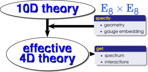
Figure 1: Orbifold model building.

Consistency conditions then limit the possible number of models to a finite number. A complete classification of all gauge embeddings has first been attempted for the $\mathbbm{Z}_{3}$ orbifold [46, 47]. The main problem is that there is a huge redundancy in the shift $V$ and Wilson lines. In orbifold models, two sets $(V,W_{\alpha})$ and $(V^{\prime},W_{\alpha}^{\prime})$ are equivalent if they are related by Weyl reflections. If they differ by vectors in the root lattice of $\mathrm{E}_{8}\times\mathrm{E}_{8}$, $\Lambda_{\mathrm{E}_{8}\times\mathrm{E}_{8}}$, they are equivalent, or fall into a small number of equivalence classes, called brother models in [48]. However, the Weyl group of $\mathrm{E}_{8}$ is enormously large, the number of elements is 696729600, so that in practice it is impossible to check whether two shifts are equivalent or not. Giedt’s method [46, 47] allows one to eliminate these redundancies to a large extent, but not completely. To obtain the true number of models, in [21] a statistical method, based on proposals made in a different context [49, 50], has been described. There shifts and Wilson lines are generated randomly, and the spectra are computed. One builds up sets of models by the following procedure: generate a first model. Then generate randomly further models and add them to the set as long as they are not already contained in this set; if the model was already present, terminate. The criterion if two models are equivalent or not is taken to be whether or not the spectra coincide; this underestimates the true number of models somewhat. The size of thus generated model sets goes as $\sqrt{N}$, where $N$ denotes the number of inequivalent models. Using this strategy, one finds that the $\mathbbm{Z}_{6}$-II orbifold admits roughly $10^{7}$ inequivalent gauge embeddings.

Let us now come to how the promising models with the exact MSSM spectra were found. The search strategy was based on the concept of LGU, as explained above. In the context of the heterotic orbifolds, this means that one should look at compactifications that exhibit fixed points with local GUT groups and localized GUT representations, which eventually give rise to complete SM representations. The simplest way to obtain a three-generation model is to look at models in which there are three fixed points with an $\mathrm{SO}(10)$ symmetry and localized $\boldsymbol{16}$-plets [51]. However, it turns out that stringy consistency conditions (such as modular invariance) are so restrictive that in all settings of this type one has to buy extra states which imply that one either has to allow for chiral exotics or play with the normalization of hypercharge, thus giving up the simple picture of MSSM gauge coupling unification [17, 18].

Since the idea of three sequential families does not work smoothly, one has to look for alternatives. The perhaps simplest possibility is to go for “$2+1$ family models”, i.e. settings where two families are explained as completely localized $\boldsymbol{16}$-plets while the third family comes from ‘somewhere else’. Models of this type have first been studied in the context of string-derived Pati-Salam models [52, 53]. In what follows, we shall focus on MSSM models with this structure [16, 17, 18, 41, 20, 54]. It turns out that $2+1$ family models are indeed promising:

1. one can find $\mathcal{O}(100)$ models with the chiral MSSM spectra, which denote the so-called “heterotic mini-landscape”;

2. exotics are vector-like w.r.t. $G_{\mathrm{SM}}$ and can be decoupled consistently with vanishing $F$- and $D$-terms;

3. these settings exhibit various additional good features automatically, i.e. one does not have to search for these features, they are simply there.

It is the last point which motivates the title of these proceedings, and which will be the focus of the subsequent discussion.

Before discussing the surprising features, let us note that, in order to get rid of the vector-like exotics, one has to switch on VEVs of certain SM singlet fields $s_{i}$. Giving VEVs to states localized at certain fixed points corresponds to resolving or ‘blowing up’ the respective singularity (for a recent discussion see [55, 56]). Often one can blow up an orbifold completely, thus arriving at a smooth Calabi-Yau space. However, in the models we shall discuss it turns out that a complete blow-up always destroys some phenomenologically important features of the models, for instance breaks hypercharge at a high scale [57]. This fact has been interpreted in different ways. The authors of [57] regard it as fine tuning if not all singularities are blown up. On the other hand, string theory is known to be well-behaved at the orbifold point since the very first papers on this subject [32]. Even more, the orbifold point denotes a symmetry-enhanced configuration in moduli space, and it is well known that moduli tend to settle at such points [58, 59] (for a recent field-theoretic example demonstrating this see [60]). This is because these are typically stationary points of the scalar potential. It is also clear that in the presence of a 4D Fayet-Iliopoulos (FI) term, not all fields can reside at the orbifold point. Instead, one has to go to a ‘nearby vacuum’ in which the FI term is canceled [61]. In such a situation, some fields get driven somewhat away from the orbifold point while other stay there. Of course, these arguments do not tell us why only some SM singlets attain VEVs, yet they might nevertheless allow us to give a preference for so-called partial against full blow-ups.

The search for MSSM models in the $\mathbbm{Z}_{6}$-II orbifold has been completed in [21]. It turns out that there are $\mathcal{O}(100)$ models without the $2+1$ family structure, still giving rise to the exact MSSM spectra. In this scan, about $5\cdot 10^{6}$ out of a total of $\sim 10^{7}$ inequivalent models has been analyzed. Most MSSM candidates are based on two and some on one local GUTs (see table 1). Interestingly, although the subset of models with 2 equivalent families, i.e. the models with two out of three possible non-trivial Wilson lines, is very small, only about $3\cdot 10^{4}$ out of $10^{7}$ models have this structure, the majority of MSSM candidates is based on 2 Wilson lines.

local GUT	“family”	2 WL	3 WL
$\mathrm{E}_{6}$	$\boldsymbol{27}$	$14$	$53$
$\mathrm{SO}(10)$	$\boldsymbol{16}$	$87$	$7$
$\mathrm{SU}(6)$	$\boldsymbol{15}$+$\boldsymbol{\bar{6}}$	$2$	$4$
$\mathrm{SU}(5)$	$\boldsymbol{10}$	$51$	$10$
rest		$39$	$0$
total		$193$	$74$

Table 1: Result of a random scan for MSSM models in the $\mathbbm{Z}_{6}$-II orbifold. “2 WL” and “3 WL” means that two or three Wilson lines are switched on.

Only a small subset of 39 candidates does not exhibit local GUT structures at all. This might be interpreted as evidence for the importance of incorporating elements of grand unification into string model building.

3 Phenomenological properties

Let us now discuss some of the most important phenomenological properties oof these models. We will mainly focus on the 2WL models, since they are, as of now, better explored. They fall into two classes, depending on the shift; it can be either

$$V_{\mathrm{KRZ}}~{}=~{}\left(\frac{1}{3},\frac{1}{3},\frac{1}{3},0,0,0,0,0\right)\left(\frac{1}{6},\frac{1}{6},0,0,0,0,0,0\right)$$ (6a)

or

$$V_{\mathrm{BHLR}}~{}=~{}\left(\frac{1}{2},\frac{1}{2},\frac{1}{3},0,0,0,0,0\right)\left(\frac{1}{3},0,0,0,0,0,0,0\right)\;.$$ (6b)

$V_{\mathrm{KRZ}}$ has been first used in the context of Pati-Salam models [52, 53] while the first MSSM models in the $\mathbbm{Z}_{6}$-II orbifold were based on $V_{\mathrm{BHLR}}$ [16, 17].

3.1 Neutrino masses

One of the most striking observations supporting the picture of the great desert between the electroweak and GUT scales comes from neutrino masses, which are known to be small,

$$m_{\nu}~{}\lesssim~{}0.1\,\mathrm{eV}\;.$$ (7)

The smallness of $m_{\nu}$ can, in a very compelling way, be related to the hierarchy between the GUT and electroweak scales. The most prominent realization is the see-saw [62], where the neutrino masses are given by the famous formula

$$m_{\nu}~{}\sim~{}\frac{v^{2}}{M_{\bar{\nu}}}$$ (8)

with $v$ and $M_{\bar{\nu}}$ denoting the electroweak VEV and the mass of right-handed neutrinos $\bar{\nu}_{i}$, respectively. Data, in particular from the atmospheric neutrino oscillations, seem to indicate that $M_{\bar{\nu}}$ has to be somewhat below the GUT scale. It turns out that the mini-landscape has a built-in mechanism to lower the see-saw scale against the mass scale of vector-like exotics, which can be argued to be of the order of the GUT or compactification scale. The mechanism relies on the presence of $\mathcal{O}(100)$ instead of three right-handed neutrinos $\bar{\nu}_{i}$. To understand this, let us explain what a neutrino in these constructions is. To be specific, we focus on vacua with matter or $R$ parity, some of which have been explored in [18, 20, 54]. A neutrino is then simply an $R$-parity odd $G_{\mathrm{SM}}$ singlet. To obtain the see-saw formula (8), one has to integrate out the right-handed neutrinos. In other words, the effective neutrino masses get contributions from all neutrinos (figure 2).

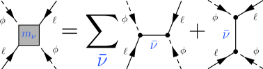
Figure 2: See-saw.

In the presence of $N_{\bar{\nu}}>3$ neutrinos, $m_{\nu}$ gets enhanced against what one gets in the the 3-neutrino case [63], with the enhancement factor going roughly as $\sqrt{N_{\bar{\nu}}}$ [64]. Because of the contributions of many neutrinos outside the $\mathrm{SO}(10)$ $\boldsymbol{16}$-plet, the flavor structure of $m_{\nu}$ is not directly related to the flavor structure of the quarks and charged leptons. To first approximation, one gets some flavor anarchy [65]; deriving reliable textures in specific vacua along the lines of [66] appears also feasible.

3.2 Flavor structure

Let us now take a closer look at the Yukawa couplings of charged fermions. Here, we focus on the $\mathcal{O}(100)$ models based on $V_{\mathrm{BHLR}}$ (equation (6b)). They turn out to have the following family structure (up to vector-like states):

• $1^{\mathrm{st}}$ and $2^{\mathrm{nd}}$ families come from $\boldsymbol{16}$-plets localized at $\mathrm{SO}(10)$ fixed points;

• $3^{\mathrm{rd}}$ family $\bar{d}$ and $\ell$ (i.e. the $3^{\mathrm{rd}}$ family $\overline{\boldsymbol{5}}$ in $\mathrm{SU}(5)$ language) come from the $T_{2/4}$ sectors and therefore correspond to states localized on two-dimensional submanifolds in compact 6D space;

• $3^{\mathrm{rd}}$ family $\bar{u}$, $\bar{e}$ and $q$ as well as the Higgs fields $h_{u}$ and $h_{d}$ are bulk fields, i.e. free to propagate everywhere in compact space.

Let us discuss implications of these facts at a naive, field-theoretic level. Yukawa couplings connecting the Higgs fields to matter may be written as overlap integrals, one could then expect that the couplings of the first two generations are suppressed by the total 6D volume while the $\tau$ and $b$ Yukawas, $y_{\tau}$ and $y_{b}$, are suppressed by the 4D volume transverse to the two-dimensional submanifold and the top Yukawa $y_{t}$ is unsuppressed, thus leading to the hierarchy

$$\text{Yukawa couplings of the first two generations}~{}\ll~{}y_{\tau},y_{b}~{}\ll~{}y_{t}\;.$$

Needless to say that this is not against data. It is somewhat surprising that, at least in the search based on local GUTs, the heterotic string did not allow us to get MSSM models with three sequential families, where the flavor structure would have been unrealistic. On the contrary, it forced us to go to models where the appearance of the third family is somewhat miraculous, but the flavor structure is qualitatively realistic.

The top Yukawa coupling $y_{t}$ plays a special role as it is directly related to the (unified) gauge coupling. At tree level, one obtains an equality between $y_{t}$ and the unified gauge coupling [41]

$$y_{t}~{}=~{}g\;.$$ (9)

This relation is subject to various corrections. Apart from the usual 4D renormalization group running, the most important modifications of this relation stem from non-trivial localization effects. To discuss these, consider an orbifold GUT limit in which the $\mathrm{SO}(4)$ plane gets large. Here, the right-handed top quark and the third generation quark doublet are contained in a hypermultiplet [41]. The two different $N=1$ components of this hypermultiplet attain different non-trivial profiles due to the presence of localized Fayet-Iliopoulos (FI) terms [67]. As a consequence, the prediction for $y_{t}$ at the compactification scale gets reduced against the gauge coupling $g$, where the suppression depends the geometry of internal space [68]. On the other hand, the value of $y_{t}$ at the compactification or GUT scale translates into a prediction for the ratio of Higgs VEVs $\tan\beta$. It turns out that the reduction is phenomenologically welcome, and allows us to obtain moderately large (or even large) $\tan\beta$, which seem to be favored by phenomenology, in particular by the LEP bound on the lightest Higgs mass. A rough estimate of the reduction seems to indicate that rather anisotropic geometries, allowing for an orbifold GUT interpretation, are favored [68].

Such anisotropic geometries allow us, at the same time, to reconcile the GUT scale with the string scale [69, footnote 3]. This can be accomplished by associating $M_{\mathrm{GUT}}$ to the inverse of the largest radius, while all (or most of) the other radii are much smaller. In this case, the volume of compact space can be small enough to ensure that the perturbative description of the setting is still appropriate. This idea has been studied in some detail more recently [70]. The outcome of the analysis is that the above puzzle can be resolved if the largest radius is by a factor 50 or so larger than the other radii. Amazingly, the estimate of the suppression of the top Yukawa coupling reveals that, in order to obtain phenomenologically attractive values for $\tan\beta$, one has to go to a rather anisotropic orbifold. This gives further support for this idea of reconciling the GUT and string scales.

Another important issue is the flavor structure of the soft supersymmetry breaking terms. The fact that the two light generations reside at two equivalent fixed points has important implications. As a consequence, the two light generations transform as a doublet under a $D_{4}$ discrete flavor symmetry [52, 75]. Therefore, the structure of the soft masses is [76]

$$\widetilde{m}^{2}~{}=~{}\left(\begin{array}[]{ccc}a&0&0\\ 0&a&0\\ 0&0&b\end{array}\right)+\text{terms proportional to $D_{4}$ breaking VEVs}\;.$$ (10)

This structure is very much reminiscent of the scheme of “minimal flavor violation” (MFV) [77, 78, 79], in which the soft masses are of the form

$$\widetilde{m}^{2}_{\mathrm{MFV}}~{}=~{}a\,\mathbbm{1}+b\,Y^{\dagger}\,Y\;.$$ (11)

Here the $Y^{\dagger}\,Y$ term represents operators built up from Yukawa matrices transforming appropriately under the classical flavor symmetry $G_{\mathrm{flavor}}~{}=~{}\mathrm{SU}(3)_{u}\times\mathrm{SU}(3)_{d}\times\mathrm{SU}(3)_{q}\times\mathrm{SU}(3)_{e}\times\mathrm{SU}(3)_{\ell}$ that appears in the SM when all Yukawas are set to zero. It turns out that, if one imposes (11) at the GUT scale, the form of $\widetilde{m}^{2}$ stays preserved under the renormalization group. Even more, the coefficients $a$ and $b$ in (11) get driven to non-trivial quasi-fixed points [80, 81], which makes it practically impossible to distinguish experimentally between zero and non-zero $b$, i.e. an mSUGRA ansatz or its MFV-inspired generalization, at the GUT scale. Moreover, the supersymmetric CP phases get driven to zero [81], thus relaxing the supersymmetric CP problems. Hence, the $D_{4}$ flavor symmetry ensures phenomenological properties very close to those of the so-called mSUGRA ansatz, which is known to evade the phenomenological constraints. In summary, the $D_{4}$ symmetry seems to represent an appropriate means to ameliorate or even avoid the supersymmetric flavor problems, without the need to rely on a specific scenario of mediation of supersymmetry breaking.

3.3 Scale of supersymmetry breakdown and moduli stabilization

This brings us to another very important question: how is supersymmetry broken and why is the weak scale so far below the scale where gauge couplings meet? The traditional answer to these questions relies on dimensional transmutation [82], i.e. supersymmetry is broken by some hidden sector that gets strong at an intermediate scale $\Lambda$. The gravitino mass, setting the scale for the MSSM soft masses, is then given by [83]

$$m_{3/2}~{}\sim~{}\frac{\Lambda^{3}}{M_{\mathrm{P}}^{2}}\;.$$ (12)

However, if one is to embed this attractive scheme into string theory, one first has to fix the moduli, in particular the dilaton, whose VEV sets the gauge coupling and thus determines the scale of hidden sector strong dynamics $\Lambda$. Often this re-introduces the problem of hierarchies. This is perhaps most transparent in the effective superpotential obtained in the framework of flux compactifications (a.k.a. KKLT [88] superpotential)

$$\mathscr{W}_{\mathrm{KKLT}}~{}=~{}c+A\,\mathrm{e}^{-a\,S}\;,$$ (13)

where $c$ is a constant and the second term represents the hidden sector strong dynamics, and $\operatorname{Re}S\propto 1/g^{2}$. In the minimum, the second term adjusts its size to $c$. In particular, the scale of the gravitino mass is set by $c$,

$$m_{3/2}~{}\sim~{}c$$ (14)

in Planck units. In the landscape picture [89, 90] $c$ happens to be small by anthropic reasons, i.e. although the natural scale for $c$ in flux compactifications is order one in Planck units, due to a huge number of vacua there are some with strongly suppressed $c$, and we happen to live in such a vacuum.

In [91] an alternative has been proposed where $c$ emerges as the VEV of the perturbative superpotential and its smallness is explained by a symmetry (and hence in agreement with the more traditional criteria of “naturalness” [92]). It turns out that $R$ symmetries allow us to control the VEV of the superpotential. First, a continuous $\mathrm{U}(1)_{R}$ implies that, for configurations that satisfy the global supersymmetry $F$ term equations of a polynomial, perturbative superpotential $\mathscr{W}_{\mathrm{pert}}$

$$F_{i}~{}:=~{}\frac{\partial\mathscr{W}_{\mathrm{pert}}}{\partial\phi_{i}}~{}=~{}0\;,$$ (15)

the expectation value of the superpotential vanishes [91],

$$\langle\mathscr{W}_{\mathrm{pert}}\rangle~{}=~{}0\;.$$ (16)

This statement holds regardless of whether $\mathrm{U}(1)_{R}$ is unbroken, where the statement is trivial, or (spontaneously) broken. Further, in the presence of an approximate $\mathrm{U}(1)_{R}$ symmetry, this statement gets modified to

$$\langle\mathscr{W}_{\mathrm{pert}}\rangle~{}\sim~{}\langle\phi\rangle^{N}\;,$$ (17)

where $N$ is the order at which explicit $R$ symmetry breaking terms appear and $\langle\phi\rangle$ denotes the typical size of field VEVs. As it turns out, orbifold models give us approximate $\mathrm{U}(1)_{R}$ symmetries. They are a consequence of exact, discrete $R$ symmetries, reflecting a discrete rotational symmetry of compact 6D space. Specifically, in the $\mathbbm{Z}_{6}$-II orbifold based on the Lie lattice $\Lambda_{\mathrm{G}_{2}\times\mathrm{SU}(3)\times\mathrm{SO}(4)}$, one has a

$$[\mathbbm{Z}_{6}\times\mathbbm{Z}_{3}\times\mathbbm{Z}_{2}]_{R}$$ (18)

symmetry [53, 93]; other orbifolds have similar discrete symmetries. Some vacua of the mini-landscape models have been analyzed; the result is that the expectation value of the perturbative superpotential is

$$\langle\mathscr{W}_{\mathrm{pert}}\rangle~{}=~{}10^{-\mathcal{O}(10)}\;.$$ (19)

Since the $R$ symmetry is only approximate, the notoriously troublesome $R$ axion is massive and therefore harmless. One retains instead an approximate $R$ axion $\eta$, whose mass is slightly enhanced against against $\langle\mathscr{W}_{\mathrm{pert}}\rangle$,

$$m_{\eta}~{}\simeq~{}\frac{\langle\mathscr{W}_{\mathrm{pert}}\rangle}{\langle\phi\rangle^{2}}\;.$$ (20)

Further, in many configurations, this is the only light mode, i.e. the curvature in all other directions is much larger. Explicit examples for simple field-theoretic toy models as well as a description of the situation for the mini-landscape models have been discussed very recently [94].

Let us comment that approximate continuous symmetries, which arise from high-power exact discrete symmetries, might also allow us to solve other fundamental problems, such as the strong CP problem [95].

The hierarchically small vacuum expectation value of the superpotential can be used in order to stabilize the dilaton [91]. One obtains an effective, KKLT-like superpotential,

$$\mathscr{W}_{\mathrm{eff}}~{}=~{}\langle\mathscr{W}_{\mathrm{pert}}\rangle+A\,\mathrm{e}^{-a\,S}+\frac{1}{2}m_{\eta}\,\eta^{2}\;,$$ (21)

which describes the ‘hidden sector’ up to heavier modes. In the supersymmetric minimum, the non-perturbative term $A\,\mathrm{e}^{-a\,S}$ adjusts its size to the VEV of the perturbative superpotential $\langle\mathscr{W}_{\mathrm{pert}}\rangle$. At this level, one obtains a vacuum with a fixed dilaton. The vacuum expectation value of the superpotential, i.e. the gravitino mass, is given by

$$m_{3/2}~{}\simeq~{}\langle\mathscr{W}_{\mathrm{eff}}\rangle~{}\sim~{}\langle\mathscr{W}_{\mathrm{pert}}\rangle\;.$$ (22)

As usual, $m_{3/2}$ will set the scale for the MSSM soft masses and the electroweak scale. One may also speculate that some hidden sector matter fields acquire $F$-terms such as to to correct the vacuum energy in the spirit of ‘$F$-term uplifting’ [97]; a possible way to stabilize the $T$-moduli has been sketched in [98]. This might then lead to a ‘mirage-like’ pattern of soft supersymmetric masses [99], and will be discussed in more detail elsewhere.

An important question concerns whether the size of the non-perturbative term is consistent with a phenomenologically viable gauge coupling $g$, i.e. whether the dilaton gets fixed at realistic values. This question can be answered affirmatively. In order to see this, let us briefly review the analysis of [19], where the scale $\Lambda$ of hidden sector strong dynamics in the mini-landscape has been studied. Here, the hidden sector is defined as the gauge group with the largest $\beta$-function coefficient. It was found that, for a realistic gauge coupling, $\Lambda$ takes values which are, by the relation (12), consistent with TeV-scale soft masses.

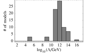
(a) 2 WL (from [19]).

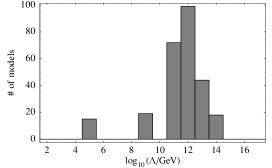
(b) 3 WL (from [21]).

Figure 3: Statistics of the scale of hidden sector gaugino condensation $\Lambda$ in (a) the heterotic mini-landscape and (b) its extension to three Wilson lines. $\Lambda$ is peaked at values, where according to (12) the soft masses are in the TeV range.

This is illustrated in figure 3, where we also show the result of the completion of the mini-landscape search [21]. These statistics show that, under the assumption of a realistic gauge coupling, $\Lambda$ is such that by relation (12) a phenomenologically attractive gravitino mass emerges. Turning this argument around, we see that once we are in a vacuum with $\langle\mathscr{W}_{\mathrm{pert}}\rangle\sim 10^{-15}$, the hidden sector $\beta$-function coefficients are such that the dilaton gets fixed at a realistic value.

The hierarchically small vacuum expectation value of $\mathscr{W}_{\mathrm{pert}}$ has important consequences for the solution of the MSSM $\mu$ problem. In these models, $\langle\mathscr{W}_{\mathrm{pert}}\rangle$ is proportional to the MSSM $\mu$ parameter [100]. This can be shown by expanding the Kähler potential [101] in the holomorphic combination $h_{u}\,h_{d}$ [94]. One then obtains a which correspond to holomorphic [102] term proportional to the VEV of the superpotential and Giudice-Masiero type [103] contribution, so altogether

$$\mu~{}\sim~{}m_{3/2}\;.$$ (23)

Taking into account both contributions, this can lead to consistent boundary conditions for the soft masses. This has been discussed recently in the framework of 5D orbifold GUTs [104], where the possible contribution of a Chern-Simons term to the $\mu$ term has been taken into account. It turns out that the Chern-Simons contribution is crucial in order to obtain a viable phenomenology [104]. It appears also interesting to see if, by having a better understanding of the origin of the MSSM $\mu$ parameter, one might be able to shed some light on the MSSM fine tuning problem.

Before summarizing the good features in the last section, let us briefly comment on open questions and potential problems. There might be a mild tension between the estimated size of the coefficients of dimension five proton decay operators and the observed proton longevity; on the other hand, we have not really obtained a full understanding of the patterns of the Yukawa couplings. It might well turn out that, once we fully understand why the $u$ and $d$ Yukawa couplings are so small, we will also be able to explain why the first generations coefficients of the $qqq\ell$ and $\bar{u}\bar{u}\bar{d}\bar{e}$ operators are highly suppressed (cf. also [105] for a recent, very similar discussion). We have further argued that highly anisotropic compactifications might allow us to reconcile the discrepancy between the string and GUT scales. However, so far we do not have obtained a dynamical mechanism that allows us to understand why there is a hierarchy between the radii. And, of course, we have not much to say on the most fundamental questions such as the observed vacuum energy.

4 Summary

In these proceedings, some progress of embedding ideas of grand unification into string theory is described. Field-theoretic orbifold GUTs provided us with the geometric intuition for how to efficiently search for realistic models. This has lead to the concept of local grand unification which gives a simple explanation for the simultaneous existence of complete GUT multiplets and split multiplets in Nature. Using this as a guideline, potentially realistic models with the exact MSSM spectra and a simple geometric interpretation have been obtained. These models have vacua with $R$ parity and are consistent with MSSM gauge coupling unification. That is, we imposed our prejudices of supersymmetry and unification in our model search, where we had to disregard models which are not consistent with our criteria. Amazingly, those of the models which survive this selection process have many unexpected features, which were not ‘put in by hand’ but happen to occur automatically. The most striking of these ‘stringy surprises’ are:

• neutrino see-saw with the see-saw scale somewhat below the GUT or compactification scale;

• “gauge-top unification” and a correlation between reasonable values for $\tan\beta$ and anisotropy of the model;

• a potential solution to the supersymmetric flavor and CP problems based on the non-Abelian discrete flavor symmetry $D_{4}$;

• high-power discrete $R$ symmetries explaining a hierarchically small gravitino mass;

• a hidden sector whose scale of strong dynamics is consistent with a TeV scale gravitino mass;

• a relation between the $\mu$ term and the scale of supersymmetry breakdown.

Future might tell us whether these are just accidents or connected to the real world.

Acknowledgments

It is a pleasure to thank F. Brümmer, W. Buchmüller, K. Hamaguchi, P. Hosteins, R. Kappl, T. Kobayashi, O. Lebedev, H.P. Nilles, P. Paradisi, F. Plöger, S. Raby, S. Ramos-Sánchez, R. Schieren, K. Schmidt-Hoberg, C. Simonetto and P. Vaudrevange for very fruitful collaborations, and K. Schmidt-Hoberg and P. Vaudrevange for comments. Further thanks go to the organizers of the Yukawa symposium for the wonderful meeting and the fantastic conference dinner. This research was supported by the DFG cluster of excellence Origin and Structure of the Universe and the SFB-Transregio 27 ”Neutrinos and Beyond” by Deutsche Forschungsgemeinschaft (DFG).

References

- [1] D. I. Olive, Invited talk given at Study Conf. on Unification of Fundamental Interactions II, Erice, Italy, Oct 6-14, 1981.
- [2] D. J. Gross, J. A. Harvey, E. J. Martinec, and R. Rohm, Phys. Rev. Lett. 54 (1985), 502–505.
- [3] D. J. Gross, J. A. Harvey, E. J. Martinec, and R. Rohm, Nucl. Phys. B256 (1985), 253.
- [4] H. P. Nilles, (2004), hep-th/0410160.
- [5] L. E. Ibáñez, (1987), Based on lectures given at the XVII GIFT Seminar on Strings and Superstrings, El Escorial, Spain, Jun 1-6, 1987 and Mt. Sorak Symposium, Korea, Jul 1987 and ELAF ’87, La Plata, Argentina, Jul 6-24, 1987.
- [6] M. Ratz, (2007), arXiv:0711.1582 [hep-ph].
- [7] H. P. Nilles, S. Ramos-Sánchez, M. Ratz, and P. K. S. Vaudrevange, Eur. Phys. J. C59 (2009), 249–267, [0806.3905].
- [8] S. Raby, Eur. Phys. J. C59 (2009), 223–247, [0807.4921].
- [9] F. Gmeiner and G. Honecker, JHEP 09 (2007), 128, [arXiv:0708.2285 [hep-th]].
- [10] F. Gmeiner and G. Honecker, JHEP 07 (2008), 052, [0806.3039].
- [11] G. B. Cleaver, (2007), hep-ph/0703027.
- [12] R. Donagi and K. Wendland, (2008), 0809.0330.
- [13] V. Bouchard and R. Donagi, Phys. Lett. B633 (2006), 783–791, [hep-th/0512149].
- [14] V. Braun, Y.-H. He, B. A. Ovrut, and T. Pantev, JHEP 05 (2006), 043, [hep-th/0512177].
- [15] J. E. Kim, J.-H. Kim, and B. Kyae, JHEP 06 (2007), 034, [hep-ph/0702278].
- [16] W. Buchmüller, K. Hamaguchi, O. Lebedev, and M. Ratz, Phys. Rev. Lett. 96 (2006), 121602, [hep-ph/0511035].
- [17] W. Buchmüller, K. Hamaguchi, O. Lebedev, and M. Ratz, Nucl. Phys. B785 (2007), 149–209, [hep-th/0606187].
- [18] O. Lebedev, H. P. Nilles, S. Raby, S. Ramos-Sánchez, M. Ratz, P. K. S. Vaudrevange, and A. Wingerter, Phys. Lett. B645 (2007), 88, [hep-th/0611095].
- [19] O. Lebedev, H. P. Nilles, S. Raby, S. Ramos-Sánchez, M. Ratz, P. K. S. Vaudrevange, and A. Wingerter, Phys. Rev. Lett. 98 (2007), 181602, [hep-th/0611203].
- [20] O. Lebedev, H. P. Nilles, S. Raby, S. Ramos-Sánchez, M. Ratz, P. K. S. Vaudrevange, and A. Wingerter, Phys. Rev. D77 (2007), 046013, [arXiv:0708.2691 [hep-th]].
- [21] O. Lebedev, H. P. Nilles, S. Ramos-Sánchez, M. Ratz, and P. K. S. Vaudrevange, Phys. Lett. B668 (2008), 331–335, [0807.4384].
- [22] Y. Kawamura, Prog. Theor. Phys. 103 (2000), 613–619, [hep-ph/9902423].
- [23] Y. Kawamura, Prog. Theor. Phys. 105 (2001), 999–1006, [hep-ph/0012125].
- [24] G. Altarelli and F. Feruglio, Phys. Lett. B511 (2001), 257–264, [hep-ph/0102301].
- [25] L. J. Hall and Y. Nomura, Phys. Rev. D64 (2001), 055003, [hep-ph/0103125].
- [26] A. Hebecker and J. March-Russell, Nucl. Phys. B613 (2001), 3–16, [hep-ph/0106166].
- [27] T. Asaka, W. Buchmüller, and L. Covi, Phys. Lett. B523 (2001), 199–204, [hep-ph/0108021].
- [28] L. J. Hall, Y. Nomura, T. Okui, and D. R. Smith, Phys. Rev. D65 (2002), 035008, [hep-ph/0108071].
- [29] G. Burdman and Y. Nomura, Nucl. Phys. B656 (2003), 3–22, [hep-ph/0210257].
- [30] M. Quiros, (2003), hep-ph/0302189.
- [31] L. J. Dixon, J. A. Harvey, C. Vafa, and E. Witten, Nucl. Phys. B261 (1985), 678–686.
- [32] L. J. Dixon, J. A. Harvey, C. Vafa, and E. Witten, Nucl. Phys. B274 (1986), 285–314.
- [33] L. E. Ibáñez, H. P. Nilles, and F. Quevedo, Phys. Lett. B187 (1987), 25–32.
- [34] L. E. Ibáñez, J. E. Kim, H. P. Nilles, and F. Quevedo, Phys. Lett. B191 (1987), 282–286.
- [35] J. A. Casas, E. K. Katehou, and C. Muñoz, Nucl. Phys. B317 (1989), 171.
- [36] J. A. Casas and C. Muñoz, Phys. Lett. B214 (1988), 63.
- [37] A. Font, L. E. Ibáñez, H. P. Nilles, and F. Quevedo, Nucl. Phys. B307 (1988), 109, Erratum ibid. B310.
- [38] A. Font, L. E. Ibáñez, H. P. Nilles, and F. Quevedo, Phys. Lett. B213 (1988), 274.
- [39] S. Förste, H. P. Nilles, P. K. S. Vaudrevange, and A. Wingerter, Phys. Rev. D70 (2004), 106008, [hep-th/0406208].
- [40] W. Buchmüller, K. Hamaguchi, O. Lebedev, and M. Ratz, (2005), hep-ph/0512326.
- [41] W. Buchmüller, C. Lüdeling, and J. Schmidt, JHEP 09 (2007), 113, [arXiv:0707.1651 [hep-ph]].
- [42] J. C. Pati and A. Salam, Phys. Rev. D10 (1974), 275–289.
- [43] J. Schmidt, (2009), 0906.5501.
- [44] P. K. S. Vaudrevange, (2008), 0812.3503.
- [45] S. Ramos-Sánchez, (2008), 0812.3560.
- [46] J. Giedt, Ann. Phys. 289 (2001), 251, [hep-th/0009104].
- [47] J. Giedt, Nucl. Phys. B671 (2003), 133–147, [hep-th/0301232].
- [48] F. Plöger, S. Ramos-Sánchez, M. Ratz, and P. K. S. Vaudrevange, JHEP 04 (2007), 063, [hep-th/0702176].
- [49] K. R. Dienes, Phys. Rev. D73 (2006), 106010, [hep-th/0602286].
- [50] K. R. Dienes and M. Lennek, Phys. Rev. D75 (2007), 026008, [hep-th/0610319].
- [51] W. Buchmüller, K. Hamaguchi, O. Lebedev, and M. Ratz, Nucl. Phys. B712 (2005), 139–156, [hep-ph/0412318].
- [52] T. Kobayashi, S. Raby, and R.-J. Zhang, Phys. Lett. B593 (2004), 262–270, [hep-ph/0403065].
- [53] T. Kobayashi, S. Raby, and R.-J. Zhang, Nucl. Phys. B704 (2005), 3–55, [hep-ph/0409098].
- [54] W. Buchmüller and J. Schmidt, Nucl. Phys. B807 (2009), 265–289, [0807.1046].
- [55] S. Groot Nibbelink, T.-W. Ha, and M. Trapletti, Phys. Rev. D77 (2008), 026002, [arXiv:0707.1597 [hep-th]].
- [56] S. Groot Nibbelink, D. Klevers, F. Plöger, M. Trapletti, and P. K. S. Vaudrevange, JHEP 04 (2008), 060, [0802.2809].
- [57] S. Groot Nibbelink, J. Held, F. Ruehle, M. Trapletti, and P. K. S. Vaudrevange, JHEP 03 (2009), 005, [0901.3059].
- [58] M. Dine, Prog. Theor. Phys. Suppl. 134 (1999), 1–17, [hep-th/9903212].
- [59] L. Kofman et al., JHEP 05 (2004), 030, [hep-th/0403001].
- [60] W. Buchmüller, R. Catena, and K. Schmidt-Hoberg, (2009), 0902.4512.
- [61] J. J. Atick, L. J. Dixon, and A. Sen, Nucl. Phys. B292 (1987), 109–149.
- [62] P. Minkowski, Phys. Lett. B67 (1977), 421.
- [63] W. Buchmüller, K. Hamaguchi, O. Lebedev, S. Ramos-Sánchez, and M. Ratz, Phys. Rev. Lett. 99 (2007), 021601, [hep-ph/0703078].
- [64] J. R. Ellis and O. Lebedev, Phys. Lett. B653 (2007), 411–418, [arXiv:0707.3419 [hep-ph]].
- [65] L. J. Hall, H. Murayama, and N. Weiner, Phys. Rev. Lett. 84 (2000), 2572–2575, [hep-ph/9911341].
- [66] A. Y. Smirnov, Phys. Rev. D48 (1993), 3264–3270, [hep-ph/9304205].
- [67] H. M. Lee, H. P. Nilles, and M. Zucker, Nucl. Phys. B680 (2004), 177–198, [hep-th/0309195].
- [68] P. Hosteins, R. Kappl, M. Ratz, and K. Schmidt-Hoberg, JHEP 07 (2009), 029, [0905.3323].
- [69] E. Witten, Nucl. Phys. B471 (1996), 135–158, [hep-th/9602070].
- [70] A. Hebecker and M. Trapletti, Nucl. Phys. B713 (2005), 173–203, [hep-th/0411131].
- [71] B. Dundee, S. Raby, and A. Wingerter, (2008), 0805.4186.
- [72] B. Dundee, S. Raby, and A. Wingerter, (2008), 0811.4026.
- [73] J. E. Kim and B. Kyae, (2007), 0712.1596.
- [74] M. A. Klaput and C. Paleani, (2010), 1001.1480.
- [75] T. Kobayashi, H. P. Nilles, F. Plöger, S. Raby, and M. Ratz, Nucl. Phys. B768 (2007), 135–156, [hep-ph/0611020].
- [76] P. Ko, T. Kobayashi, J.-h. Park, and S. Raby, Phys. Rev. D76 (2007), 035005, [arXiv:0704.2807 [hep-ph]].
- [77] R. S. Chivukula and H. Georgi, Phys. Lett. B188 (1987), 99.
- [78] A. J. Buras, P. Gambino, M. Gorbahn, S. Jäger, and L. Silvestrini, Phys. Lett. B500 (2001), 161–167, [hep-ph/0007085].
- [79] G. D’Ambrosio, G. F. Giudice, G. Isidori, and A. Strumia, Nucl. Phys. B645 (2002), 155–187, [hep-ph/0207036].
- [80] P. Paradisi, M. Ratz, R. Schieren, and C. Simonetto, Phys. Lett. B668 (2008), 202–209, [0805.3989].
- [81] G. Colangelo, E. Nikolidakis, and C. Smith, Eur. Phys. J. C59 (2009), 75–98, [0807.0801].
- [82] E. Witten, Nucl. Phys. B188 (1981), 513.
- [83] H. P. Nilles, Phys. Lett. B115 (1982), 193.
- [84] N. V. Krasnikov, Phys. Lett. B193 (1987), 37–40.
- [85] P. Binétruy, M. K. Gaillard, and Y.-Y. Wu, Nucl. Phys. B481 (1996), 109–128, [hep-th/9605170].
- [86] J. A. Casas, Phys. Lett. B384 (1996), 103–110, [hep-th/9605180].
- [87] M. K. Gaillard and B. D. Nelson, Int. J. Mod. Phys. A22 (2007), 1451, [hep-th/0703227].
- [88] S. Kachru, R. Kallosh, A. Linde, and S. P. Trivedi, Phys. Rev. D68 (2003), 046005, [hep-th/0301240].
- [89] F. Quevedo, Phys. World 16N11 (2003), 21–22.
- [90] L. Susskind, (2003), hep-th/0302219.
- [91] R. Kappl, H. P. Nilles, S. Ramos-Sánchez, M. Ratz, K. Schmidt-Hoberg, and P. K. Vaudrevange, Phys. Rev. Lett. 102 (2009), 121602, [0812.2120].
- [92] G. ’t Hooft, NATO Adv. Study Inst. Ser. B Phys. 59 (1980), 135.
- [93] T. Araki, K.-S. Choi, T. Kobayashi, J. Kubo, and H. Ohki, (2007), arXiv:0705.3075 [hep-ph].
- [94] F. Brümmer, R. Kappl, M. Ratz, and K. Schmidt-Hoberg, (2010), 1003.0084.
- [95] K.-S. Choi, H. P. Nilles, S. Ramos-Sánchez, and P. K. S. Vaudrevange, (2009), 0902.3070.
- [96] S. Weinberg, Rev. Mod. Phys. 61 (1989), 1–23.
- [97] O. Lebedev, H. P. Nilles, and M. Ratz, Phys. Lett. B636 (2006), 126–131, [hep-th/0603047].
- [98] B. Dundee, S. Raby, and A. Westphal, (2010), 1002.1081.
- [99] V. Löwen and H. P. Nilles, Phys. Rev. D77 (2008), 106007, [0802.1137].
- [100] J. A. Casas and C. Muñoz, Phys. Lett. B306 (1993), 288–294, [hep-ph/9302227].
- [101] I. Antoniadis, E. Gava, K. S. Narain, and T. R. Taylor, Nucl. Phys. B432 (1994), 187–204, [hep-th/9405024].
- [102] J. E. Kim and H. P. Nilles, Phys. Lett. B138 (1984), 150.
- [103] G. F. Giudice and A. Masiero, Phys. Lett. B206 (1988), 480–484.
- [104] F. Brümmer, S. Fichet, A. Hebecker, and S. Kraml, JHEP 08 (2009), 011, [0906.2957].
- [105] C. Smith, (2008), 0809.3152.