Binary black hole merger in the extreme-mass-ratio limit: a multipolar analysis.

Abstract

Building up on previous work, we present a new calculation of the gravitational wave emission generated during the transition from quasi-circular inspiral to plunge, merger and ringdown by a binary system of nonspinning black holes, of masses $m_{1}$ and $m_{2}$, in the extreme mass ratio limit, $m_{1}m_{2}\ll(m_{1}+m_{2})^{2}$. The relative dynamics of the system is computed without making any adiabatic approximation by using an effective one body (EOB) description, namely by representing the binary by an effective particle of mass $\mu=m_{1}m_{2}/(m_{1}+m_{2})$ moving in a (quasi-)Schwarzschild background of mass $M=m_{1}+m_{2}$ and submitted to an ${\cal O}(\nu)$ 5PN-resummed analytical radiation reaction force, with $\nu=\mu/M$. The gravitational wave emission is calculated via a multipolar Regge-Wheeler-Zerilli type perturbative approach (valid in the limit $\nu\ll 1$). We consider three mass ratios, $\nu=\{10^{-2},10^{-3},10^{-4}\}$, and we compute the multipolar waveform up to $\ell=8$. We estimate energy and angular momentum losses during the quasiuniversal and quasigeodesic part of the plunge phase and we analyze the structure of the ringdown. We calculate the gravitational recoil, or “kick”, imparted to the merger remnant by the gravitational wave emission and we emphasize the importance of higher multipoles to get a final value of the recoil $v/(c\nu^{2})=0.0446$. We finally show that there is an excellent fractional agreement ($\sim 10^{-3}$) (even during the plunge) between the 5PN EOB analytically-resummed radiation reaction flux and the numerically computed gravitational wave angular momentum flux. This is a further confirmation of the aptitude of the EOB formalism to accurately model extreme-mass-ratio inspirals, as needed for the future space-based LISA gravitational wave detector.

I Introduction

After the breakthroughs of 2005 Pretorius:2005gq ; Campanelli:2005dd ; Baker:2005vv , state-of-the-art numerical relativity (NR) codes can nowadays routinely evolve (spinning) coalescing binary black hole systems with comparable masses and extract the gravitational wave (GW) signal with high accuracy Hannam:2007ik ; Hannam:2007wf ; Sperhake:2008ga ; Campanelli:2008nk ; Scheel:2008rj ; Chu:2009md ; Mosta:2009rr ; Pollney:2009yz . However, despite these considerable improvements, the numerical computation of coalescing black hole binaries where the mass ratio is considerably different from 1:1 is still challenging. To date, the mass ratio 10:1 (without spin) remains the highest that was possible to numerically evolve through the transition from inspiral to plunge and merger with reasonable accuracy Gonzalez:2008bi ; Lousto:2010tb . In recent years, work at the interface between analytical and numerical relativity, notably using the effective-one-body (EOB) resummed analytical formalism Buonanno:1998gg ; Buonanno:2000ef ; Damour:2000we ; Damour:2001tu ; Buonanno:2005xu ; Damour:2009ic , has demonstrated the possibility of using NR results to develop accurate analytical models of dynamics and waveforms of coalescing black-hole binaries Buonanno:2007pf ; Damour:2007yf ; Damour:2007vq ; Damour:2008te ; Boyle:2008ge ; Buonanno:2009qa ; Damour:2009kr ; Pan:2009wj ; Barausse:2009xi .

By contrast, when the mass ratio is large, approximation methods based on black-hole perturbation theory are expected to yield accurate results, therefore enlarging our black-hole binaries knowledge by a complementary perspective. In addition, when the larger black-hole mass is in the range $10^{5}M_{\odot}$-$10^{7}M_{\odot}$, the GWs emitted by the radiative inspiral of the small object fall within the sensitivity band of the proposed space-based detector LISA lisa1 ; lisa2 , so that an accurate modelization of these extreme-mass-ratio-inspirals (EMRI) is one of the goals of current GW research.

The first calculation of the complete gravitational waveform emitted during the transition from inspiral to merger in the extreme-mass-ratio limit was performed in Refs. Nagar:2006xv ; Damour:2007xr , thanks to the combination of 2.5PN Padé resummed radiation reaction force Damour:1997ub with Regge-Wheeler-Zerilli perturbation theory Regge:1957td ; Zerilli:1970se ; Nagar:2005ea ; Martel:2005ir . This test-mass laboratory was then used to understand, element by element, the physics that enters in the dynamics and waveforms during the transition from inspiral to plunge (followed by merger and ringdown), providing important inputs for EOB-based analytical models. In particular, it helped to: (i) discriminate between two expressions of the resummed radiation reaction force; (ii) quantify the accuracy of the resummed multipolar wavefom; (iii) quantify the effect of non-quasi-circular corrections (both to waveform and radiation reaction); (iv) qualitatively understand the process of generation of quasi-normal modes (QNMs); and (v) improve the matching procedure of the “insplunge” waveform to a “ringdown” waveform with (several) QNMs. In the same spirit, the multipolar expansion of the gravitational wave luminosity of a test-particle in circular orbits on a Schwarzschild background Cutler:1993vq ; Yunes:2008tw ; Pani:2010em was helpful to devise an improved resummation procedure Damour:2007yf ; Damour:2008gu of the PN (Taylor-expanded) multipolar waveform Kidder:2007rt ; Blanchet:2008je . Such resummation procedure is one of the cardinal elements of what we think is presently the best EOB analytical model Damour:2009kr ; Pan:2009wj . Similarly, Ref. Yunes:2009ef compared “calibrated” EOB-resummed waveforms Boyle:2008ge with Teukolsky-based perturbative waveforms, and confirmed that the EOB framework is well suited to model EMRIs for LISA.

In addition, recent numerical achievement in the calculation of the conservative gravitational self-force (GSF) of circular orbits in a Schwarzschild background Detweiler:2008ft ; Barack:2009ey ; Barack:2010tm prompted the interplay between post-Newtonian (PN) and GSF efforts Blanchet:2009sd ; Blanchet:2010zd , and EOB and GSF efforts Damour:2009sm . In particular, the information coming from GSF data helped to break the degeneracy (among some EOB parameters) which was left after using comparable-mass NR data to constrain the EOB formalism Damour:2009sm . (See also Ref. Barausse:2009xi for a different way to incorporate GSF results in EOB).

In this paper we present a revisited computation of the GWs emission from the transition from inspiral to plunge in the test-mass limit. We improve the previous calculation of Nagar et al. Nagar:2006xv in two aspects: one numerical and the other analytical. The first is that we use a more accurate (4th-order) numerical algorithm to solve the Regge-Wheeler-Zerilli equations numerically; this allows us to capture the higher order multipolar information (up to $\ell=8$) more accurately than in Nagar:2006xv . The second aspect is that we have replaced the 2.5PN Padé resummed radiation reaction force of Nagar:2006xv with the 5PN resummed one that relies on the results of Ref. Damour:2008gu .

The aim of this paper is then two-fold. On the one hand, our new test-mass perturbative allows us to describe in full, and with high accuracy, the properties of the gravitational radiation emitted during the transition inspiral-plunge-merger and ringdown, without making the adiabatic approximation which is the hallmark of most existing approaches to the GW emission by EMRI systems Glampedakis:2002cb ; Hughes:2005qb . We compute the multipolar waveform up to $\ell=8$, we discuss the relative weight of each multipole during the nonadiabatic plunge phase, and describe the structure of the ringdown. In addition, from the multipolar waveform we compute also the total recoil, or kick, imparted to the system by the wave emission, thereby complementing NR results Gonzalez:2008bi . On the other hand, we can use our upgraded test-mass laboratory to provide inputs for the EOB formalism, notably for completing the EOB multipolar waveform during the late-inspiral, plunge and merger. As a first step in this direction, we show that the analytically resummed radiation reaction introduced in Damour:2008gu ; Damour:2009kr gives an excellent fractional agreement ($\sim 10^{-3}$) with the angular momentum flux computed á la Regge-Wheeler-Zerilli even during the plunge phase.

This paper is organized as follows. In Sec. II we give a summary of the formalism employed. In Sec. III we describe the multipolar structure of the waveforms; details on the energy and angular momentum emitted during the plunge-merge-ringdown transition are presented as well as an analysis of the ringdown phase. Section IV is devoted to present the computation of the final kick, emphasizing the importance of high multipoles. The following Sec. V is devoted to some consistency checks: on the one hand, we discuss the aforementioned agreement between the mechanical angular momentum loss and GW energy flux during the plunge; on the other hand, we investigate the influence of EOB “self-force” terms (either in the conservative and non conservative part of the dynamics) on the waveforms. We present a summary of our findings in Sec. VI. In Appendix A we supply some technical details related to our numerical framework, while in Appendix B we list some useful numbers. We use geometric units with $c=G=1$.

II Analytic framework

II.1 Relative dynamics

The relative dynamics of the system is modeled specifying the EOB dynamics to the small-mass limit. The formalism that we use here is the specialization to the test-mass limit of the improved EOB formalism introduced in Ref. Damour:2009kr that crucially relies on the “improved resummation” procedure of the multipolar waveform of Ref. Damour:2008gu . Let us recall that the EOB approach to the general relativistic two-body dynamics is a nonperturbatively resummed analytic technique which has been developed in Refs. Buonanno:1998gg ; Buonanno:2000ef ; Damour:2000we ; Damour:2001tu ; Buonanno:2005xu . This technique uses, as basic input, the results of PN theory, such as: (i) PN-expanded equations of motion for two pointlike bodies, (ii) PN-expanded radiative multipole moments, and (iii) PN-expanded energy and angular momentum fluxes at infinity. For the moment, the most accurate such results are the 3PN conservative dynamics Damour:2001bu ; Blanchet:2003gy , the 3.5PN energy flux Blanchet:2001aw ; Blanchet:2004bb ; Blanchet:2004ek for the $\nu\neq 0$ case, and 5.5PN Tanaka:1997dj accuracy for the $\nu=0$ case. Then the EOB approach “packages” this PN-expanded information in special resummed forms which extend the validity of the PN results beyond the expected weak-field-slow-velocity regime into (part of) the strong-field-fast-motion regime. In the EOB approach the relative dynamics of a binary system of masses $m_{1}$ and $m_{2}$ is described by a Hamiltonian $H_{\rm EOB}(M,\mu)$ and a radiation reaction force ${\cal F}_{\rm EOB}(M,\mu)$, where $M\equiv m_{1}+m_{2}$ and $\mu\equiv m_{1}m_{2}/M$. In the general comparable-mass case $H_{\rm EOB}$ has the structure $H_{\rm EOB}(M,\mu)=M\sqrt{1+2\nu(\hat{H}_{\nu}-1)}$ where $\nu\equiv\mu/M\equiv m_{1}m_{2}/(m_{1}+m_{2})^{2}$ is the symmetric mass ratio. In the test mass limit that we are considering, $\nu\ll 1$, we can expand $H_{\rm EOB}$ in powers of $\nu$. After subtracting inessential constants we get a Hamiltonian per unit ($\mu$) mass $\hat{H}=\lim_{\nu\to 0}(H-{\rm const.})/\mu=\lim_{\nu\to 0}\hat{H}_{\nu}$. As in Refs. Nagar:2006xv ; Damour:2007xr , we replace the Schwarzschild radial coordinated $r_{*}=r+2M\log[r/(2M)-1]$ and, correspondingly, the radial momentum $P_{R}$ by the conjugate momentum $P_{R_{*}}$ of $R_{*}$, so that the specific Hamiltonian has the form

$$\hat{H}=\sqrt{A\left(1+\frac{p_{\varphi}^{2}}{\hat{r}^{2}}\right)+p_{r_{*}}^{2}}\ .$$ (1)

Here we have introduced dimensionless variables ${\hat{r}}\equiv R/M$,${\hat{r}}_{*}\equiv R_{*}/M$, $p_{r_{*}}\equiv P_{R_{*}}/\mu$, $p_{\varphi}\equiv P_{\varphi}/(\mu M)$ and $A=1-2/{\hat{r}}$. Hamilton’s canonical equations for $({\hat{r}},r_{*},p_{r_{*}},p_{\varphi})$ in the equatorial plane ($\theta=\pi/2$) yield

$$\dot{{\hat{r}}}_{*} =\dfrac{p_{{\hat{r}}_{*}}}{\hat{H}}\ ,$$ (2)

$$\dot{{\hat{r}}} =\dfrac{A}{\hat{H}}p_{r_{*}}\equiv v_{r}\ ,$$ (3)

$$\dot{\varphi} =\dfrac{A}{\hat{H}}\dfrac{p_{\varphi}}{{\hat{r}}^{2}}\equiv\Omega\ ,$$ (4)

$$\dot{p}_{r_{*}} =-\dfrac{{\hat{r}}-2}{{\hat{r}}^{3}\hat{H}}\left[p_{\varphi}^{2}\left(\dfrac{3}{{\hat{r}}^{2}}-\dfrac{1}{{\hat{r}}}\right)+1\right]\ ,$$ (5)

$$\dot{p}_{\varphi} =\hat{\cal F}_{\varphi}\ .$$ (6)

Note that the quantity $\Omega$ is dimensionless and represents the orbital frequency in units of $1/M$. In these equations the extra term $\hat{\cal F}_{\varphi}$ [of order $O(\nu)$] represents the non conservative part of the dynamics, namely the radiation reaction force. Following Damour:2006tr ; Nagar:2006xv ; Damour:2007xr , we use the following expression:

$$\hat{{\cal F}}_{\varphi}\equiv-\dfrac{32}{5}\nu\Omega^{5}{\hat{r}}^{4}\hat{f}_{\rm DIN}(v_{\varphi}),$$ (7)

where $v_{\varphi}=\hat{r}\Omega$ is the azimuthal velocity and $\hat{f}_{\rm DIN}=F^{\ell_{\rm max}}/F_{\rm Newt}$ denotes the (Newton normalized) energy flux up to multipolar order $\ell_{\rm max}$(in the $\nu=0$ limit) resummed according to the “improved resummation” technique of Ref. Damour:2008gu . This resummation procedure is based on a particular multiplicative decomposition of the multipolar gravitational waveform. The energy flux is written as

$$F^{\ell_{\rm max}}=\dfrac{1}{8\pi}\sum_{\ell=2}^{\ell_{\rm max}}\sum_{m=1}^{\ell}(m\Omega)^{2}|rh_{\ell m}|^{2}.$$ (8)

where $h_{\ell m}$ is the factorized waveform of Damour:2008gu ,

$$h_{\ell m}=h_{\ell m}^{(N,\epsilon)}\hat{S}_{\rm eff}^{(\epsilon)}T_{\ell m}e^{{\rm i}\delta_{\ell m}}\rho^{\ell}_{{\ell m}}$$ (9)

where $h_{\ell m}^{(N,\epsilon)}$ represents the Newtonian contribution given by Eq. (4) of Damour:2008gu , $\epsilon=0$ (or $1$) for $\ell+m$ even (odd), $\hat{S}^{\epsilon}_{\rm eff}$ is the effective “source”, Eqs. (15-16) of Damour:2008gu ; $T_{\ell m}$ is the “tail factor” that resums an infinite number of “leading logarithms” due to tail effects, Eq. (19) of Damour:2008gu ; $\delta_{\ell m}$ is a residual phase correction, Eqs. (20-28) of Damour:2008gu ; and $\rho_{\ell m}$ is the residual modulus correction, Eqs. (C1-C35) in Damour:2008gu . In our setup we truncate the sum on $\ell$ at $\ell_{\rm max}=8$. We refer the reader to Fig. 1 (b) of Damour:2008gu to figure out the capability of the new resummation procedure to reproduce the actual flux (computed numerically) for the sequence of circular orbits in Schwarzshild.

II.2 Gravitational wave generation

The computation of the gravitational waves generated by the relative dynamics follows th same line of Refs. Nagar:2006xv ; Damour:2007xr , and relies on the numerical solution, in the time domain, of the Regge-Wheeler-Zerilli equations for metric perturbations of the Schwarzschild black hole with a point-particle source. Once the dynamics from Eqs. (2)-(6) is computed, one needs to solve numerically (for each multipole $(\ell,m)$ of even (e) or odd (o) type) a couple of decoupled partial differential equations

$$\partial_{t}^{2}\Psi^{(\rm e/o)}_{\ell m}-\partial_{r_{*}}^{2}\Psi^{(\rm e/o)}_{\ell m}+V^{(\rm e/o)}_{\ell}\Psi^{(\rm e/o)}_{\ell m}=S^{(\rm e/o)}_{\ell m}\$$ (10)

with source terms $S^{(\rm e/o)}_{\ell m}$ linked to the dynamics of the binary. Following Nagar:2006xv , the sources are written in the functional form

$$S^{(\rm e/o)}_{\ell m} =G^{(\rm e/o)}_{\ell m}(r,t)\delta(r_{*}-R_{*}(t))$$

$$+F^{(\rm e/o)}_{\ell m}(r,t)\partial_{r_{*}}\delta(r_{*}-R_{*}(t))\ ,$$ (11)

with $r$-dependent [rather than $R(t)$-dependent] coefficients $G(r)$ and $F(r)$. The explicit expression of the sources is given in Eqs. (20-21) of Nagar:2006xv , to which we address the reader for further technical details. We mention, however, that in our approach the distributional $\delta$-function is approximated by a narrow Gaussian of finite width $\sigma\ll M$. In Ref. Nagar:2006xv it was already pointed out that, if $\sigma$ is sufficiently small and the resolution is sufficiently high (so that the Gaussian can be cleanly resolved) this approximation is competitive with other approaches that employ a mathematically more rigorous treatment of the $\delta$-function Lousto:1997wf ; Martel:2001yf ; Sopuerta:2005gz (see in this respect Table 1 and Fig. 2 of Ref. Nagar:2006xv ). That analysis motivates us to use the same representation of the $\delta$-function also in this paper, but together with an improved numerical algorithm to solve the wave equations. In fact, the solution of Eqs. (10) is now provided via the method of lines by means of a 4th-order Runge-Kutta algorithm with 4th-order finite differences used to approximate the space derivatives. This yields better accuracy in the waveforms (using resolutions comparable to those of Ref. Nagar:2006xv ), and allows to better resolve the higher multipoles. More details about the numerical implementation, convergence properties, accuracy, and comparison with published results are given in Appendix A.

From the numerically calculated master functions $\Psi^{(\rm e/o)}_{\ell m}$, one can then obtain, when considering the limit $r\to\infty$, the $h_{+}$ and $h_{\times}$ gravitational-wave polarization amplitude

$$h_{+}-{\rm i}h_{\times}=\dfrac{1}{r}\sum_{\ell\geq 2,m}\sqrt{\frac{(\ell+2)!}{(\ell-2)!}}\left(\Psi^{(\rm e)}_{\ell m}+{\rm i}\Psi^{(\rm o)}_{\ell m}\right)\;_{-2}Y^{\ell m}\ ,$$ (12)

where $\;{}_{-2}Y^{\ell m}\equiv\,_{-2}Y^{\ell m}(\theta,\varphi)$ are the $s=2$ spin-weighted spherical harmonics goldberg67 . From this expression, all the interesting second-order quantities follow. The emitted power,

$$\dot{E}=\frac{1}{16\pi}\sum_{\ell\geq 2,m}\frac{(\ell+2)!}{(\ell-2)!}\left(\left|\dot{\Psi}^{(\rm o)}_{\ell m}\right|^{2}+\left|\dot{\Psi}^{(\rm e)}_{\ell m}\right|^{2}\right)\;,\\$$ (13)

the angular momentum flux

$$\dot{J}=\frac{1}{32\pi}\sum_{\ell\geq 2,m}\bigg{\{}{\rm i}m\frac{(\ell+2)!}{(\ell-2)!}\left[\dot{\Psi}^{(\rm e)}_{\ell m}\Psi^{(\rm e)*}_{\ell m}+\dot{\Psi}_{\ell m}^{({\rm o})}\Psi^{(\rm o)*}_{\ell m}\right]+c.c.\bigg{\}}\\$$ (14)

and the linear momentum flux Thorne:1980ru ; Pollney:2007ss ; Ruiz:2007yx

$${\cal F}^{\bf P}_{x}+{\rm i}{\cal F}^{\bf P}_{y} =\dfrac{1}{8\pi}\sum_{\ell\geq 2,m}\bigg{[}{\rm i}a_{{\ell m}}\dot{\Psi}_{{\ell m}}^{({\rm e})}\dot{\Psi}^{({\rm o})*}_{\ell,m+1}$$

$$+b_{{\ell m}}\left(\dot{\Psi}^{(\rm e)}_{{\ell m}}\dot{\Psi}^{(\rm e)*}_{\ell+1,m+1}+\dot{\Psi}^{(\rm o)}_{{\ell m}}\dot{\Psi}^{(\rm o)*}_{\ell+1,m+1}\right)\bigg{]}\ .$$ (15)

with

$$a_{{\ell m}} =2(\ell-1)(\ell+2)\sqrt{(\ell-m)(\ell+m+1)}$$ (16)

$$b_{\ell m} =\dfrac{(\ell+3)!}{(\ell+1)(\ell-2)!}\sqrt{\dfrac{(\ell+m+1)(\ell+m+2)}{(2\ell+1)(2\ell+3)}}.$$ (17)

III Relative dynamics and waveforms

Figure 1: Transition from quasicircular inspiral orbit to plunge. Initial position is $r_{0}=7M$ and $\nu=10^{-3}$.

Let us now consider the dynamics and waveforms obtained within our new setup. Evidently, at the qualitative level our results are analogous to those of Refs. Nagar:2006xv ; Damour:2007xr . By contrast, at the quantitative level, dynamics and waveforms are slightly different due to the new, more accurate, radiation reaction force. The particle is initially at $r=7M$. The dynamics is initiated with the so called post-circular initial data for ($p_{\varphi}$,$p_{r}$) introduced in Ref. Buonanno:2000ef and specialized to the $\mu\to 0$ limit (see Eqs. (9)-(13) of Ref. Nagar:2006xv ). Because of the smallness of the value of $\mu$ we are using, this approximation is sufficient to guarantee that the initial eccentricity is negligible. To have a better modelization of the extreme-mass-ratio limit regime we considered three values of the mass ratio $\nu$, namely $\nu=\{10^{-2},\,10^{-3},\,10^{-4}\}$. The values of $\nu$ are chosen so that the particle passes through a long (when $\nu\leq 10^{-3}$) quasicircular adiabatic inspiral before entering the nonadiabatic plunge phase. Fig 1 displays the relative trajectory for $\nu=10^{-3}$. The system executes about 40 orbits before crossing the LSO at $r=6M$ while plunging into the black hole.

Figure 2: Complete $\ell=m=2$ gravitational (Zerilli) waveform corresponding to the dynamics depicted in Fig. 1. The waveform is extracted at $r_{*}^{\rm obs}/M=1000$.

The main multipolar contribution to the gravitational signal is clearly the $\ell=m=2$. The real part of the corresponding waveform is displayed in Fig. 2. It is extracted at $r_{*}^{\rm obs}=1000M$ and it is shown versus observer’s retarded time $u=(t^{\rm obs}-r_{*}^{\rm obs})M$. Note how the amplitude of the long wavetrain emitted during the adiabatic quasicircular inspiral grows very slowly for about $4000M$, until the transition from inspiral to plunge around the crossing of the adiabatic LSO frequency. In the following we want however to focus on the higher order multipolar contributions to the waveform, as they are particularly relevant in our test-mass setup. The computation of these multipoles and their inclusion in the analysis is one of the new results of this paper .

Figure 3 summarizes the information a bout the multipolar waveforms up to $\ell=8$. The left panels show the moduli (normalized by the mass ratio $\nu$), while the right panels show the corresponding instantaneous gravitational wave frequencies $M\omega_{\ell m}$. We show, for each value of $\ell$, the dominant (even-parity) ones, i.e. those with $m=\ell$, together with some subdominant (odd-parity) ones. The comparison between the moduli highlights how the amplitude of higher modes, that is almost negligible during the adiabatic inspiral, can be magnified of about factor two (see the $\ell=2$, $m=1$ case) or three (see the $m=\ell=6$ case) during the nonadiabatic plunge phase. This fact is expected to have some relevance in those computations that are dominated by the nonadiabatic plunge phase, like the computation of the recoil velocity imparted to the center of mass of the system due to the linear momentum carried away by GWs Damour:2006tr . As we will see in Sec. IV, high-order multipoles are, in fact, needed to obtain an accurate result. An analysis of the relative importance of the different multipoles based on energy considerations is the subject of Sec. III.1.

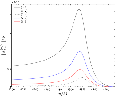
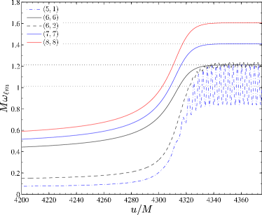
Figure 3: Multipolar structure of the waveform. The left panels exhibit the moduli; the right panels the instantaneous gravitational wave frequencies for some representative multipoles. Note the oscillation pattern during ringdown (especially in the $\ell=2$, $m=1$ modulus and frequency) due to the interference between positve and negative frequency QNMs. The waveform refer to the $\nu=10^{-3}$ mass ratio.

As for the instantaneous GW frequency, the right-panels of Fig. 3 show the same kind of behavior for each multipole: $M\omega_{\ell m}$ is approximately equal to $m\Omega$ during the inspiral, to grow abruptly during the nonadiabatic plunge phase until it saturates at the ringdown frequency (indicated by dashed lines in the plot). As already pointed out in Ref. Nagar:2006xv ; Damour:2007xr the oscillation pattern that is clearly visible for some multipoles is due to the contemporary (but asymmetric) excitation of the positive and negative frequency QNMs of the black hole. We shall give details on this phenomenon in Sec. III.2.

III.1 quasiuniversal plunge

In this section we discuss in quantitative terms the relative contribution of each multipole during the plunge, merger and ringdown phase. The analysis is based on the energy and angular momentum computed from the emitted GW. While these quantities represent a “synthesis” of the information we need, their computation and interpretation have some subtle points that are discussed below.

For a (adiabatic) sequence of circular orbits, this information was originally obtained in Cutler et al. Cutler:1993vq ; for the radial plunge of a particle initially at rest at infinity, the classical work of Davis, Ruffini, Press and Price Davis:1971gg found that about the $90\%$ of the total energy is quadrupole ($\ell=2$) radiation, and about the $8\%$ is octupole ($\ell=3$) radiation. Concerning the transition from quasicircular inspiral to plunge, Ref. Nagar:2006xv performed a (preliminary) calculation of the total energy and angular momentum losses during a “plunge” phase (that was defined by the condition $r<5.9865M$, with $\nu=0.01$) followed by merger and ringdown, computing all the multipolar contributions up to $\ell=4$ (see Table 2 in Nagar:2006xv ).

We will follow up and improve the calculation of Ref. Nagar:2006xv . Let us first point out some conceptual difficulties. As a matter of fact, any kind of computation of the losses during the transition from inspiral to plunge in our setup will depend both on the value of $\nu$, and on the initial time from which one starts the integration of the fluxes (for instance on the time when one defines the beginning of the “plunge” phase). It follows that, if robust and meaningful results are desired, the calculation has to be focused on the part of the waveforms that is quasiuniversal (i.e., with negligible dependence on $\nu$). As was pointed out in Nagar:2006xv , the quasiuniversal behavior reached in the $\nu\to 0$ limit is linked to the quasigeodesic character of the plunge motion, which approaches the geodesic which starts from the LSO in the infinite past with zero radial velocity.

In this respect, let us recall that, as shown in Ref. Buonanno:2000ef , the transition from the adiabatic inspiral to the nonadiabatic plunge is not sharp, but rather blurred, namely it occurs in a radial domain around the LSO which scaled with $\nu$ as $r-6M\sim\alpha M\nu^{2/5}$, with the radial velocity scaling as $v_{r}\sim-\beta\nu^{3/5}$. In practical terms, this means that the quasiuniversal, quasigeodesic plunge does not really start at $r_{0}=6M$, but at about $r_{0}/M\sim 6-\alpha\nu^{2/5}$. In Ref. Buonanno:2000ef , using a 2.5PN Padé resummed radiation reaction, the coefficients $\alpha$ and $\beta$ were determined to be $\alpha_{\rm 2.5PN}=1.89$ and $\beta_{\rm 2.5PN}=-0.072$. However, since our setup is based on the 5PN resummed radiation reaction force, we do not expect those numbers to remain unchanged, so that they do not represent for us a reliable estimate to extract the part of the waveforms we are interested in. Taking a pragmatical approach, we can determine this quasiuniversal region by contrasting our simulations at different $\nu$, so to see when the dependence on $\nu$ is sufficiently “small” (say at $1\%$ level in the energy and angular momentum losses, see below).

Figure 4, displays the “convergence” to the $\ell=m=2$ modulus (upper panel) and frequency (lower panel) for the three values of $\nu$. For convenience the waveforms have been time-shifted so that the maxima of the waveform mudulus (located at $u-u_{\rm max}=0$ in the figure) coincide. The plot clearly shows that the late-time part of the waveform has a converging trend to some “universal” pattern that progressively approximates the “exact” $\nu=0$ case. Note that, at the visual level, amplitudes and frequencies for $\nu=\{10^{-3}\,10^{-4}\}$ look barely distinguishable during the late part of the plunge, entailing a very weak dependence on the properties of radiation reaction. From this analysis we can assume a quasiuniversal and quasigeodesic plunge starting at about $u-u_{\rm max}=-50$ (vertical dashed line), which corresponds to $M\omega_{22}\simeq 0.167$, which is about $1.23\times(2\Omega_{\rm LSO})$ (for reference, we indicate with a horizontal line the $2\Omega_{\rm LSO}$ frequency in the lower panel of the figure) . We integrate the multipolar energy and angular momentum fluxes from $u-u_{\rm max}=-50M$ onwards and sum over all the multipoles up to $\ell=8$. The outcome of this computation is listed in Table 1 for the $\nu=\{10^{-3},\,10^{-4}\}$. Note that the agreement of these numbers at the level of $1\%$ is a good indication of the quasigeodesic character of the dynamics behind the part of the waveform that we have selected. The numerical information of Table 1 is completed by Tables 9-10 in Appendix B, were we list the values and the relative weight of each partial multipolar contribution. Coming thus to the main conclusion of this analysis, it turns out that the $\ell=m=2$ multipole contributes to the total energy (angular momentum) for about the $58\%$ ($62\%$), the $\ell=m=3$ for about the $20\%$ ($20\%$) , the $\ell=m=4$ for about the $8\%$ ($7.6\%$) and the $\ell=m=5$ for the $3.5\%$ ($3.3\%$). For what concerns the odd-parity multipole, the dominant one, $\ell=2$, $m=1$, contributes to $4.3\%$ of the total energy and $2.3\%$ of the total angular momentum. We address again the reader to Appendix B for the fully precise quantitative information.

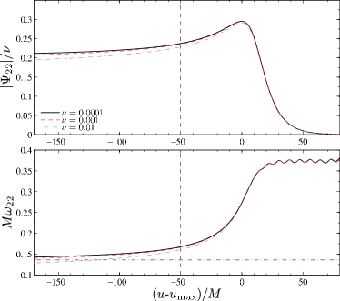
Figure 4: “Convergence” of the waveform when $\nu\to 0$. Retarded times have been shifted so that the zero coincides with the maximum of the waveform modulus $|\Psi^{(\rm e)}_{22}|$ for each value of $\nu$. The horizontal dashed line indicates the adiabatic LSO frequency. The vertical dashed line conventionally identifies the beginning of an approximately quasiuniversal and quasigeodesic plunge phase.

III.2 Ringdown

Let us focus now on the analysis of the waveform during pure ringdown only. Our main aim here is to extract quantitative information from the oscillations that are apparent in the gravitational wave frequency (and modulus) during ringdown (see Fig. 3). As explained in Sec. IIIB of Ref. Damour:2007xr , the physical interpretation of this phenomenon is clear, namely it is due to an asymmetric excitation of the positive and negative QNM frequencies of the black hole triggered by the “sign” of the particle motion (clockwise or counterclockwise). The modes that have the same sign of $m\Omega$ are the dominant ones, while the others with opposite sign are less excited (smaller amplitude). Since QNMs are basically excited by a resonance mechanism, their strength (amplitude) for a given multipole $(\ell,m)$ depends on their “distance” to the critical (real) exciting frequency $m\Omega_{\rm max}$ of the source, where $\Omega_{\rm max}$ indicates the maximum of the orbital frequency. In our setup, the particle is inspiralling counterclockwise (i.e., $\Omega>0$), therefore the positive frequency QNMs are more excited than the negative frequency ones. The amount of (relative) excitation will depend on $m$. Such QNM “interference” phenomenon was noted and explained already in Refs. Nagar:2006xv ; Damour:2007xr , although no quantitative information was actually extracted from the numerical data. We perform here this quantitative analysis.

Table 1: Total energy and angular momentum emitted during the quasiuniversal, quasigeodesic plunge phase, the merger and ringdown (it is defined by the condition $M\omega_{22}\gtrsim 0.167$, see Fig. 4 ).

$\nu$	$M\Delta E/\mu^{2}$	$\Delta J/\mu^{2}$
$10^{-3}$	0.47688	3.48918
$10^{-4}$	0.47097	3.44271

The waveform during the ringdown has the structure

$$\Psi_{{\ell m}}^{(\rm e/o)}=\sum_{n}C_{\ell mn}^{+}e^{-\sigma^{+}_{\ell n}t}+\sum_{n}C_{\ell mn}^{-}e^{-\sigma^{-}_{\ell n}t},$$ (18)

were we use the notation of Refs. Damour:2006tr ; Damour:2007xr , and denote the QNM complex frequencies with $\sigma_{\ell n}^{\pm}=\alpha_{\ell n}\pm\omega_{\ell n}$ and $C^{\pm}_{\ell mn}$ the corresponding complex amplitudes. For each value of $\ell$, $n$ indicates the order of the mode, $\alpha_{\ell n}$ its inverse damping time and $\omega_{\ell n}$ its frequency. For example, defining $a_{\ell mn}e^{{\rm i}{\vartheta}_{\ell mn}}\equiv C^{-}_{\ell mn}/C^{+}_{\ell mn}$, in the presence of only one QNM (e.g., the fundamental one, $n=0$) the instantaneous frequency computed from Eq. (18) reads

$$\omega_{{\ell m}}^{(\rm e/o)} = -\Im\left(\frac{\dot{\Psi}_{\ell m}^{(\rm e/o)}}{\Psi_{\ell m}^{(\rm e/o)}}\right)$$

$$= \frac{\left(1-a_{\ell m0}^{2}\right)\omega_{\ell 0}}{1+a_{\ell m0}^{2}+2a_{\ell m0}\cos\left(2\omega_{\ell 0}t+\vartheta_{\ell m0}\right)}.$$

This simple formula illustrates that, if the two modes are equally excited ($a_{\ell 0}=1$) then there is a destructive interference and the instantaneous frequency is zero; on the contrary, if one mode (say the positive one) is more excited than the other, the instantaneous frequency oscillates around a constant value that asymptotically tends to $\omega^{+}_{\ell 0}$ when $C_{\ell m0}^{-}\rightarrow 0$. In general, one can use a more sofisticated version of Eq. (III.2), that includes various overtones for a given multipolar order, as a template to fit the instantaneous GW frequency and to measure the various $a_{\ell mn}$ and $\vartheta_{\ell mn}$ during the ringdown. For simplicity, we concentrate here only on the measure of $a_{\ell m0}$, and we use directly Eq. (III.2). To perform such a fit (with a least-square method) we consider only the part of the ringdown that is dominated by the fundamental (least-damped) QNM; i.e., the “plateau of oscillations” approximately starting at $u/M=4340$ in the right-panels of Fig. 3.

Table 2: Fit of QNM interference with Eq. (III.2) for a representative sample of multipoles. The numbers refer to $\nu=10^{-2}$. The $M\omega_{\ell 0}$ column lists the values of the fundamental QNMs frequencies gathered from the literature Chandrasekhar:1975zza ; Chandrasekhar:1985kt ; Leaver:1985ax ; Berti:2005ys (see also Ref. Berti:2009kk for a recent review and for highly accurate computations). By contrast, the primed values are obtained from our numerical data by fitting the ringdown frequency for both $a_{\ell m0}$ and $M\omega_{\ell 0}$. Note the good consistency between the two methods.

$\ell$	$m$	$a_{\ell m0}$	$a^{\prime}_{\ell m0}$	$M\omega_{\ell 0}$	$M\omega^{\prime}_{\ell 0}$
2	1	7.2672$\times 10^{-2}$	7.2678$\times 10^{-2}$	0.37367	0.37369
2	2	4.8476$\times 10^{-3}$	4.848$\times 10^{-3}$	0.37367	0.37361
3	1	9.3403$\times 10^{-2}$	9.3403$\times 10^{-2}$	0.59944	0.59944
3	2	8.008$\times 10^{-3}$	$8.011\times 10^{-3}$	0.59944	0.59936
3	3	5.5471$\times 10^{-4}$	5.5477$\times 10^{-4}$	0.59944	0.59943
4	1	9.1560$\times 10^{-2}$	9.1559$\times 10^{-2}$	0.80917	0.80918
4	2	9.1433$\times 10^{-3}$	9.1435$\times 10^{-3}$	0.80917	0.80917
4	3	9.0473$\times 10^{-4}$	9.0475$\times 10^{-4}$	0.80917	0.80917
4	4	6.382$\times 10^{-5}$	6.379$\times 10^{-5}$	0.80917	0.80918

The fundamental frequency $n=0$ has been used as given input, and we fit for the amplitude ratio $a_{\ell m0}$ and relative phase $\theta_{\ell m0}$. The outcome of the fit for some multipoles is exhibited in Table 2. Note that in the third and fourth column we list also the values that one obtains by fitting also for the frequency $\omega_{\ell 0}^{\prime}$. We obtain perfectly consistent results. Note that for the multipole $\ell=8$ we were obliged to compute the frequency only in this way, since we could not find this number in the results of Berti:2009kk : we obtain the value $M\omega_{80}=1.60619$. The table quantifies that the strongest interference pattern, that always occurs for $m=1$ (for any $\ell$), corresponds to a relative contribution of the negative frequency mode of the order of about $9\%$. This trend remains true for all values of $\ell$. For example, we have $a_{810}=9.54\times 10^{-2}$ and $a_{710}=9.48\times 10^{-2}$. Note finally that the presence of the negative mode for the $\ell=2$, $m=1$ shows up also in the corresponding modulus $|\Psi_{21}|/\nu$, with the characteristic oscillating pattern superposed to the exponential decay (see top-left panel of Fig. 3). [See also Ref. Hadar:2009ip for an analytical treatment of the ringdown excitation amplitudes during the plunge].

IV Gravitational recoil

Let us now come to the computation of the gravitational recoil, or “kick”, imparted to the system due to the anisotropic emission of gravitational radiation. The calculation of these kicks in general relativity has been carried out in a variety of ways, that before 2005 relied mainly on analytical and semianalytical techniques. In particular, let us mention that, after the pioneering calculation of Fitchett Fitchett:1983 and Fitchett and Detweiler Fitchett:1984qn , earlier estimates included a perturbative calculation Favata:2004wz , a close-limit calculation Sopuerta:2006wj and a post-Newtonian calculation valid during the inspiral phase only Blanchet:2005rj . This latter calculation has been recently improved by bringing together post-Newtonian theory and the close limit approximation, yielding close agreement with purely NR results LeTiec:2009yg . In addition, a first attempt to compute the final kick within the EOB approach Damour:2006tr yielded the analytical understanding (before any numerical result were available) of the qualitative behavior of the kick velocity (notably the so-called “antikick” phase), as driven by the intrinsically nonadiabatic character of the plunge phase. Such preliminary EOB calculation was then improved in Schnittman:2007sn , which included also inputs from NR simulations. On the numerical side, after the pioneering computation of Baker et al. Baker:2006vn , there has been a plethora of computations of the kick from spinning black holes binaries, focusing in particular on the so-called superkick configurations. By contrast, for the nonspinining case, Refs. Gonzalez:2006md ; Gonzalez:2008bi represent to date the largest span of mass ratios for which the final kick velocity is known (see also Ref. Pollney:2007ss for the nonprecessing, equal-mass spinning case). In addition, the use of semianalytical models prompted a deeper understanding of the structure of the gravitational recoil as computed in NR simulations Schnittman:2007ij . However, despite all these numerical efforts, to date there are no “numerical” computations of the final recoil velocity in the $\nu\to 0$ limit: the only estimates rely on fits to NR data of the form

$$v^{\rm kick}=A\nu^{2}\sqrt{1-4\nu}(1+B\nu)\ ,$$ (20)

with the coefficient $A$ giving the extrapolated value in the $\nu\to 0$ limit Gonzalez:2006md ; Gonzalez:2008bi . The aim of this section is to provide a value of $A$ that comes from an actual (numerical) computation within perturbation theory.

It is convenient to treat the kick velocity vector imparted to the system by GW emission as a complex quantity, i.e. $v\equiv v_{x}+{\rm i}v_{y}$. By integrating Eq. (II.2) in time and by changing the sign, the (complex) velocity accumulated by the system up to a certain time $t$ is given by

$$v\equiv v_{x}+{\rm i}v_{y}=-\dfrac{1}{M}\int_{-\infty}^{t}\left({\cal F}_{x}^{\bf P}+{\rm i}{\cal F}_{y}^{\bf P}\right)dt^{\prime}.$$ (21)

Since in practical situations one is always dealing with a finite timeseries for the linear momentum flux, it is not possible to begin the integration from $t=-\infty$, but rather at a finite initial time $t_{0}$. This then amounts in the need of fixing some (vectorial) integration constant $v_{0}$ that accounts for the velocity that the system has acquired in evolving from $t=-\infty$ to $t=t_{0}$, i.e.

$$v=v_{0}-\dfrac{1}{M}\int_{t_{0}}^{t}\left({\cal F}_{x}^{\bf P}+{\rm i}{\cal F}_{y}^{\bf P}\right)dt.$$ (22)

As it was emphasized in Ref. Pollney:2007ss , the proper inclusion of $v_{0}$ is crucial to get the correct (monotonic) qualitative and quantitative behavior of the time evolution of the magnitude $|v|$ of the recoil velocity. Typically, not only the final value of $|v|$ may be wrong of about a $10\%$, but one can also have spurious oscillations in $|v|$ during the inspiral phase if $v_{0}$ is not properly determined or simply set to zero. See in this respect Sec. IVA of Ref. Pollney:2007ss .

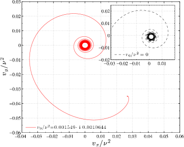
Figure 5: Parametric plot of $v_{x}$ versus $v_{y}$ (for $\nu=10^{-3}$) obtained from Eq. (22) with $v_{0}/\nu^{2}=(1.549-{\rm i}1.0644)\times 10^{-3}$. The analogous plot with $v_{0}=0$ is shown in the inset.

As in Ref. Pollney:2007ss , the numerical determination of $v_{0}$ can be done with the help of the “hodograph”, i.e., a parametric plot of the instantaneous velocity vector in the complex velocity plane $(v_{x},v_{y})$. This hodograph is displayed in Fig. 5 for $\nu=10^{-3}$. Let us focus first on the inset, that exhibits the outcome of the time integration with $v_{0}=0$. Note that the center of the inspiral (corresponding to the velocity accumulated during the quasiadiabatic inspiral phase) is displaced with respect to the correct value $v=(0,0)$, corresponding to $v_{0}=0$ at $t=-\infty$. The initial $v_{x}^{0}$ and $v_{y}^{0}$ are determined as the translational “shifts” that one needs to add (in both $v_{x}$ and $v_{y}$) so that the “center” of this inspiral is approximately zero. The result of this operation led (for $\nu=10^{-3}$) to $v_{x}^{0}/\nu^{2}=1.1549\times 10^{-3}$ and $v_{y}^{0}/\nu^{2}=-1.0644\times 10^{-3}$; this is displayed in the main panel of Fig. 5.

This judicious choice of the integration constant is such that the modulus $|v|=\sqrt{v_{x}^{2}+v_{y}^{2}}$ of the accumulated recoil velocity grows essentially monotonically in time and no spurious oscillations are present during the inspiral phase. This is emphasized by Fig. 6. In the figure, we show, as a solid line, the modulus of the total accumulated kick velocity versus observer’s retarded time (as before, waveforms are extracted at $r_{*}^{\rm obs}/M=1000$). This “global” computation is done including in the sum of Eq. (II.2) all the partial multipolar contribution up to $\ell=7$ (which actually means considering also the interference terms between $\ell=7$ and $\ell=8$ modes). To guide the eye, we added a vertical dashed line locating the maximum of $|\Psi^{(\rm e)}_{22}|$, that approximately corresponds to the dynamical time when the particle crosses the light-ring. Note the typical shape of $|v|$, with a clean local maximum and the so-called “antikick” behavior, that is qualitatively identical to the corresponding curves computed (for different mass ratios) by NR simulations (see for example Fig. 1 of Ref. Schnittman:2007ij for the 2:1 mass ratio case).

In addition to the total recoil magnitude computed up to $\ell=7$, we display on the same plot also the “partial” contribution, i.e. computations of $|v|$ where we truncate the sum over $\ell$ in Eq. (II.2) at a given value $\ell^{*}<7$. In the figure we show (depicted as various type of nonsolid lines) the evolution of recoil with $2\leq\ell^{*}\leq 6$.

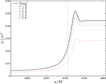
Figure 6: Time-evolution of the magnitude of the recoil velocity. The figure shows the monotonic “multipolar” convergence to the final result. The plot refers to mass ratio $\nu=10^{-3}$.

Note that each partial-$\ell$ contribution to the linear momentum flux has been integrated in time (with the related choice of integration constants) before performing the vectorial sum to obtain the total $v$. The fact that each curve nicely grows monotonically without spurious oscillations during the late-inspiral phase is a convincing indication of the robustness of the procedure we used to determine $v_{0}^{\ell^{*}}$ by means of hodographs.

Table 3: Magnitude of the final and maximum kick velocities for the three values of $\nu$ considered. The last row lists the values extrapolated to $\nu=0$ from $\nu=\{10^{-3},10^{-4}\}$ data.

$\nu$	$|v^{\rm end}|/\nu^{2}$	$|v^{\rm max}|/\nu^{2}$
$10^{-2}$	0.043234	0.050547
$10^{-3}$	0.044401	0.052058
$10^{-4}$	0.044587	0.052298
0	0.0446	0.0523

The figure highlights at a visual level the influence of high multipoles to achieve an accurate results. To give some meaningful numbers, if we consider $\ell^{*}=6$, we obtain $|v_{6}^{\rm fin}|/\nu^{2}=0.0437$ (i.e. $1.7\%$ difference), while $|v_{5}^{\rm fin}|/\nu^{2}=0.0424$ ($4.5\%$ difference).

The information conveyed by Fig. 6 is completed by Table 3, where we list the final value of the modulus of the recoil velocity of the center of mass $|v^{\rm end}|/\nu^{2}$ (as well as the corresponding maximum value $|v^{\rm max}|/\nu^{2}$) obtained in our setup for the three values of $\nu$ that we have considered. The computation of the kick for the other values of $\nu$ is procedurally identical and thus we show only the final numbers. The good agreement between the three numbers is consistent with the interpretation that the recoil is almost completely determined by the nonadiabatic plunge phase of the system (as emphasized in Ref. Damour:2006tr ), and thus it is almost unaffected by the details of the inspiral phase. Because of the late-plunge consistency between waveforms that we showed above for $\nu=\{10^{-3},\,10^{-4}\}$, we have decided to extrapolate the corresponding values of the kick for $\nu=0$. The corresponding numbers are listed (in bold) in the last row of Table 3.

Table 4: Recoil velocities in the test-mass limit obtained by (extrapolating) different finite-mass results. Our “best” value is shown in bold. See text for explanations.

Reference	$|v^{\rm end}|/\nu^{2}$
González et al. Gonzalez:2006md	0.04
Damour and Gopakumar Damour:2006tr	[0.010, 0.035]
Schnittman and Buonanno Schnittman:2007sn	[0.018, 0.041]
Sopuerta et al. Sopuerta:2006wj	[0.023, 0.046]
Le Tiec, Blanchet and Will LeTiec:2009yg	0.032
This work	0.0446

In Table 4 we compare the value of the final recoil with that (extrapolated to the test-mass limit) obtained from NR simulations Gonzalez:2006md and with semianalytical or seminumerical predictions, like the EOB Damour:2006tr ; Schnittman:2007sn , the close-limit approximation Sopuerta:2006wj (that all give a range, with rather large error bars) and the recent calculation of Le Tiec et al. LeTiec:2009yg based on a hybrid post-Newtonian-close-limit calculation

We conclude this section by discussing in more detail the comparison of our result with the NR-extrapolated value. Since the NR-extrapolated value that we list in Table 4 was obtained using only the data of Ref. Gonzalez:2006md (without the 10:1 mass ratio simulation of Gonzalez:2008bi ), we have decided to redo the fit with all the NR data together (that have been kindly given to us by the Authors). To improve the sensitivity of the fit when $\nu$ gets small, we first factor out the $\nu^{2}$ dependence in the data (i.e., we consider $v^{\rm NR}/\nu^{2}$, by continuity with the test-mass result). We then fit the data with the function

$$\tilde{f}(\nu)=A\sqrt{1-4\nu}\left(1+B\nu\right)\ .$$ (23)

Table 5 displays the results of the fit obtained using: the NR data of Ref. Gonzalez:2006md (consistent with the published result), first row; the joined information of Refs. Gonzalez:2006md ; Gonzalez:2008bi , second row; and the NR data of Gonzalez:2006md ; Gonzalez:2008bi together with the test-mass result calculated in this paper. Note that the NR fit are perfectly consistent with the test-mass value: in particular, our extrapolated value $|v^{\rm end}|/\nu^{2}=0.0446$ shows an agreement of $1.5\%$ with the value of $A$ obtained from the fit to the most complete NR information (in bold in Table 5).

The information of the table is completed by Fig. 7, that displays $\tilde{f}(\nu)$ (as a dash-dot line) obtained from the complete NR data of Refs. Gonzalez:2006md ; Gonzalez:2008bi . Note the visual good agreement between this extrapolation and the test-mass point when $\nu\to 0$. For contrast, we also show on the plot (as a dashed line) the outcome of the fit with the simple Newtonian-like formula ($B=0$) Fitchett:1983 . We also tested the effect of adding a quadratic correction [i.e. a term $C\nu^{2}$ in the polynomial multiplying the square root in $\tilde{f}(\nu)$], but we found that it does not really improve the description of the data.

Table 5: Fit coefficients for the final magnitude of the kick velocity from NR simulations as a function of $\nu$, Eq. (23). See text for discussion.

Data	$A$	$B$
González et al. Gonzalez:2006md	0.04070	-0.9883
González et al. Gonzalez:2006md ; Gonzalez:2008bi	0.04396	-1.3012
González et al. Gonzalez:2006md ; Gonzalez:2008bi + This work	0.04446	-1.3482

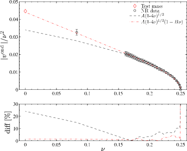
Figure 7: Results of the fit of NR data of Refs. Gonzalez:2006md ; Gonzalez:2008bi using Eq. (23). Note the good agreement between the NR-extrapolation and our test-mass result. The bottom panel contains the relative difference with the data. This plot corresponds to the second row of Table 5, without the test-mass point. See text for details.

V Consistency checks

In this section, we finally come to the discussion of some internal consistency checks of our approach. These consist in: (i) the verification of the consistency between the mechanical angular momentum loss (as driven by our analytical, resummed radiation reaction force) and the actual gravitational wave energy flux computed from the waves (as a follow up of a similar analysis done in Ref. Damour:2007xr ); (ii) a brief analysis of the influence on the (quadrupolar) waveform of the higher-order $\nu$-dependent EOB corrections entering the conservative and nonconservative part of the relative dynamics.

V.1 Angular momentum loss

One of the results of Ref. Damour:2007xr was about the comparison between the mechanical angular momentum loss provided by the resummed radiation reaction $\hat{{\cal F}}_{\varphi}$ and the angular momentum flux computed from the multipolar waveform. At that time, the main focus of Ref. Damour:2007xr was on to use of the “exact” instantaneous gravitational wave angular momentum flux $\dot{J}$ [see Eq. (14)], to discriminate between two different expression of the 2.5PN Padé resummed angular momentum flux ${\cal F}_{\varphi}^{\rm 2.5PN}$ that are degenerate during the adiabatic early inspiral. In addition , in that setup it was also possible to: (i) check consistency between $\dot{J}$ and $-{\cal F}_{\varphi}$ during the inspiral and early plunge; (ii) argue that non-quasicircular corrections in the radiation reaction are present to produce a good agreement between the “analytical” and the exact angular momentum fluxes also during the plunge, almost up to merger and (iii) show that the “exact” flux is practically insensitive to (any kind of) NQC corrections. Since we are now using a new radiation reaction force with respect to Ref. Damour:2007xr , it is interesting to redo the comparison between the Regge-Wheeler-Zerilli “exact” flux and the “analytical” mechanical loss computed along the relative dynamics.

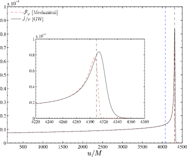
Figure 8: Comparison between two angular momentum losses: the GW flux (solid line) computed à la Regge-Wheeler-Zerilli including up to $\ell=8$ radiation multipoles, and the mechanical angular momentum loss $-{\cal F}_{\varphi}$ (dash line). The two vertical lines correspond (from left to right) to the particle crossing respectively the adiabatic LSO location ($r=6M$) and the light-ring location ($r=3M$). The plot refers to $\nu=10^{-3}$.

The result of this comparison is displayed in Fig. 8, that is the analogous of (part of) Fig. 2 of Ref. Damour:2007xr . We show in the figure the mechanical angular momentum loss (changed of sign) $-\hat{{\cal F}}_{\varphi}/\nu$ versus the mechanical time $t/M$ together with the instantaneous angular momentum flux $\dot{J}/\nu$ (computed from $\Psi^{(\rm e/o)}_{{\ell m}}$ including all contributions up to $\ell=8$) versus observer’s retarded time. Note that we did not introduce here a possible shift between the mechanical time $t$ and observer’s retarded time $u$. As such a shift is certainly expected to exist, our results should be viewed as giving a lower bound on the agreement between ${\cal F}_{\varphi}$ and $\dot{J}$. Note the very good visual agreement, not only above the LSO (vertical dashed line) but also below the LSO, and actually almost during the entire plunge phase. In fact, the accordance between the two fluxes is actually visually very good almost up to the merger (approximately identified by the maximum of the $\ell=m=2$ waveform, see dash-dot line in the inset).

We inspect this agreement at a more quantitative level in Fig. 9, where we plot the (relative) difference between $\dot{J}/\nu$ and $-\hat{{\cal F}}_{\varphi}/\nu$ versus (twice) the orbital frequency. The inset shows the relative difference from initial frequency to $2\Omega_{\rm max}$, where $\Omega_{\rm max}$ is the maximum of the orbital frequency. The main panel is a close-up centered around the LSO frequency.

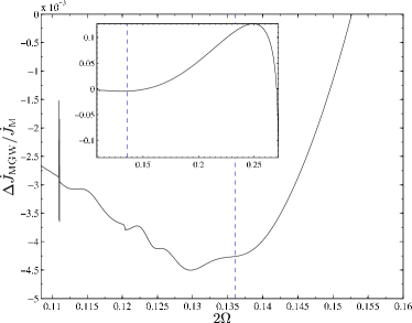
Figure 9: Difference between mechanical angular momentum loss and GW energy flux shown versus twice the orbital frequency $2\Omega$. The vertical line locates the adiabatic LSO frequency. The main panel focuses on the inspiral phase, while the inset shows the full range until the $2\Omega_{\rm max}$, where $\Omega_{\rm max}$ indicates the maximum of orbital frequency.

Note that the relative difference is of the order of $10^{-3}$ during the late inspiral and the plunge, increasing at about only a $10\%$ just before merger. We have performed the same analysis for $\nu=10^{-2}$ and $\nu=10^{-4}$, obtaining similar results. This is an indication that we have reached the limit of accuracy of our resummation procedure, limit that evidently is more apparent during the late part of the plunge. It is however remarkable that the fractional different is so small, confirming the validity of the improved $\rho$-resummation of Ref. Damour:2008gu . In this respect, we mention in passing that this fractional difference can be made even smaller by further Padé resumming the residual amplitude corrections $\rho_{\ell m}$ in a proper way. This route was explored in Ref. Damour:2008gu for the $\rho_{22}$ amplitude, yielding indeed better agreement with the “exact” circularized waveform amplitude. A more detailed analysis of these delicate issues lies out of the purpose of this paper, but will be investigated in future work.

V.2 Influence of dynamical “self-force” $\nu$-dependent effects on the waveforms.

In the work that we have presented so far we have included in the relative dynamics only the leading order part of the radiation reaction force, namely the one proportional to $\nu$. This allowed us to compute, consistently as shown above, Regge-Wheeler-Zerilli-type waveforms. In doing so we have neglected all the finite-$\nu$ effects that are important in the (complete) EOB description of the two-body problem, that is: (i) $\nu$-dependent corrections to the conservative part of the dynamics and (ii) higher order $\nu$ dependent corrections in the nonconservative part of the dynamics, i.e. corrections entering in the definition of the angular momentum flux $\hat{{\cal F}}_{\varphi}$.

In this section we want to quantify the effects entailed by these corrections on our result. To do so, we switch on the “self-force” $\nu$-dependent corrections in the Hamiltonian and in the flux defining the complete EOB relative dynamics and we compute EOB waveforms for $\nu=\{10^{-2},10^{-3},10^{-4}\}$. Since this analysis aims at giving us only a general quantitative idea of the effect of “self-force” corrections, we restrict ourself only to the computation of the $\ell=m=2$ “insplunge” waveform, without the matching to QNMs Damour:2009kr . Note also that we neglect the non-quasi-circular corrections advocated in Eq. (5) of Damour:2009kr . (See also Ref. Damour:2009ic ).

Table 6: Accumulated phase difference (computed from $\omega_{1}=0.10799$ up to $\omega_{2}\equiv 2\Omega_{\rm LSO}=0.13608$ ) [in radians] between $\ell=m=2$ EOB waveforms. $\Delta\phi_{\rm LSO}^{\rm EOB_{5PN}}$ is the phase difference accumulated between the EOB_5PN and the EOB_testmass insplunge waveforms, while $\Delta\phi_{\rm LSO}^{\rm EOB_{\rm 1PN}}$ is the phase difference accumulated between the EOB_1PN and the EOB_testmass insplunge waveforms. See text for more precise explanations.

$\nu$	$\Delta\phi_{\rm LSO}^{\rm EOB_{5PN}}$ [rad]	$\Delta\phi_{\rm LSO}^{\rm EOB_{1PN}}$ [rad]
$10^{-2}$	3.2	0.40
$10^{-3}$	3.8	0.43
$10^{-4}$	4.1	0.44

For each value of $\nu=\{10^{-2},10^{-3},10^{-4}\}$, we compute three insplunge $h_{22}$ resummed waveforms with increasingly physical complexity. The first, EOB_testmass insplunge waveform, is obtained within the ${\cal O}(\nu)$ approximation used so far; i.e., we set to zero all the $\nu$ dependent EOB corrections in $H_{\rm EOB}$ and in the normalized flux, $\hat{f}_{\rm DIN}\equiv\hat{f}_{\rm DIN}(v_{\varphi};\nu=0)$. The second, EOB_5PN insplunge waveform, is computed from the full EOB dynamics, with the complete $H_{\rm EOB}$ and $\nu$-dependent (Newton normalized) flux $\hat{f}_{\rm DIN}(v_{\varphi};\nu)$ replaced in Eq. 7. The radial potential $A(u;a_{5},a_{6},\nu)$ is given by the Padé resummed form of Eq. (2) of Ref. Damour:2009kr and $a_{5}$ and $a_{6}$ are EOB flexibility parameters that take into account 4PN and 5PN corrections in the conservative part of the dynamics. They have been constrained by comparison with numerical results Damour:2009kr ; Damour:2009sm . Following Damour:2009sm , we use here the values $a_{5}=-22.3$ and $a_{6}=+252$ as “best choice”. The third, EOB_1PN insplunge waveform, is obtained by keeping the same flux $\hat{f}_{\rm DIN}(v_{\varphi};\nu)$ of the EOB_5PN case, but only part of the EOB Hamiltonian. More precisely, we restrict the effective Hamiltonian $\hat{H}_{\rm eff}$ at 1PN level. This practically means using $A(r;0)\equiv 1-2M/r$ and dropping the $p_{r_{*}}^{4}/r^{2}$ correction term that enters in $\hat{H}_{\rm eff}$ at the 3PN level. See Eq. (1) in Damour:2009sm . We compute the relative phase difference, accumulated between frequencies $(\omega_{1},\omega_{2})$, between the EOB_testmass waveform and the other two. We chose $\omega_{1}=0.10799$, that corresponds to the initial (test-mass) GW frequency, and $\omega_{2}=2\Omega_{\rm LSO}\simeq 0.13608$. Instead of comparing the waveforms versus time, we found it convenient to do the following comparison versus frequency. For each waveform, we compute the following auxiliar quantity

$$Q_{\omega}=\dfrac{\omega^{2}}{\dot{\omega}}.$$ (24)

This quantity measures the effective number of GW cycles spent around GW frequency $\omega$ (and correspondingly weighs the signal-to-noise ratio Damour:2000gg ), and is a useful diagnostics for comparing the relative phasing accuracy of various waveforms DNTrias . Then, the gravitational wave phase $\phi_{(\omega_{1},\omega_{2})}$ accumulated between frequencies $(\omega_{1},\omega_{2})$ is given by

$$\phi_{(\omega_{1},\omega_{2})}=\int_{\omega_{1}}^{\omega_{2}}Q_{\omega}d\log\omega.$$ (25)

We can then define the relative dephasing accumulated between two waveforms as

$$\Delta\phi_{(\omega_{1},\omega_{2})}^{{\rm EOB}_{n{\rm PN}}}=\int_{\omega_{1}}^{\omega_{2}}\Delta Q_{\omega}^{{\rm EOB}_{n{\rm PN}}}d\log(\omega),$$ (26)

where $\Delta Q_{\omega}^{{\rm EOB}_{n{\rm PN}}}\equiv Q_{\omega}^{{\rm EOB}_{n{\rm PN}}}-Q_{\omega}^{\rm EOB_{testmass}}$. The results of this comparison are contained in Table 6. Note the influence of the correction due to the conservative part of the self force. Since this correction changes the location of the adiabatic $r$-LSO position Buonanno:1998gg , it entails a larger effect on the late-time portion of the binary dynamics and waveforms, resulting in a more consistent dephasing.

VI Conclusions

We have presented a new calculation of the gravitational wave emission generated through the transition from adiabatic inspiral to plunge, merger and ringdown of a binary systems of nonspinning black holes in the extreme mass ratio limit. We have used a Regge-Wheeler-Zerilli perturbative approach completed by leading order EOB-based radiation reaction force. With respect to previous work, we have improved (i) on the numerical algorithm used to solve the Regge-Wheeler-Zerilli equations and (ii) on the analytical definition of the improved EOB-resummed radiation reaction force.

Our main achievements are listed below.

1. We computed the complete multipolar waveform up to multipolar order $\ell=8$. We focused on the relative impact (at the level of energy and angular momentum losses) of the subdominant multipoles during the part of the plunge that can be considered quasiuniversal (and quasigeodesic) in good approximation. We analyzed also the structure of the ringdown waveform at the quantitative level. In particular, we measured the relative amount of excitation of the fundamental QNMs with positive and negative frequency. We found that, for each value of $\ell$, the largest excitation of the negative modes always occurs for $m=1$ and is of the order of $9\%$ of the corresponding positive mode.

2. The central numerical result of the paper is the computation of the gravitational recoil, or kick, imparted to the center of mass of the system due to the anisotropic emission of gravitational waves. We have discussed the influence of high modes in the multipolar expansion of the recoil. We showed that one has to consider $\ell\geq 4$ to have a $\sim 10\%$ accuracy in the final kick. We found for the magnitude of the final and maximum recoil velocity the values $|v^{\rm end}|/\nu^{2}=0.0446$ and $|v^{\rm max}|/\nu^{2}=0.0523$. The value of the final recoil shows a remarkable agreement ($<2\%$) with the one extrapolated from a sample of NR simulations, $|v^{\rm end}_{\rm NR}|/\nu^{2}\simeq 0.0439$.

3. The “improved resummation” for the radiation reaction used in this paper yields a better consistency agreement between mechanical angular momentum losses and gravitational wave energy flux than the previously employed Padé resummed procedure. In particular, we found an agreement between the angular momentum fluxes of the order of $0.1\%$ during the plunge (well below the LSO), with a maximum disagreement of the order of $10\%$ reached around the merger. This is a detailed piece of evidence that EOB waveforms computed via the resummation procedure of Damour:2008gu can yield accurate input for LISA-oriented science.

While writing this paper, we became aware of a similar calculation of the final recoil by Sundararajan, Khanna and Hughes PKH . Their calculation is based on a different method to treat the transition from inspiral to plunge (see Refs. Sundararajan:2007jg ; Sundararajan:2008bw ; Sundararajan:2008zm and references therein). In the limiting case of a nonspinning binary, their results for the final and maximum kick are fully consistent with ours.

Appendix A Numerical framework, tests and comparison with the literature

The numerical procedure adopted is similar to the one of Ref. Nagar:2006xv , but it has been improved on several aspects. In particular, the original code has been fully rewritten and optimized and a new finite-differencing algorithm to solve the Regge-Wheeler-Zerilli equation has been implemented.

The Regge-Wheeler-Zerilli equations, Eqs. (10), are solved as a first-order-in-time second-order-in-space system adopting the method of lines. Time advancing is done by means of a 4th order Runge-Kutta algorithm, while centered 4th order finite differences are used to approximate the space derivative. Standard Sommerfeld-maximally dissipative boundary conditions are adopted and implemented as described in Calabrese:2005fp

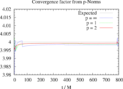
Figure 10: Self-convergence factor computed from $p$-norms of $(\ell=8,m=8)$ inspiral plunge waveforms. Resolutions used are: $\Delta r_{*}=\{0.05,\,0.025,\,0.0125\}$. The particle is initially at $R(0)=6.5M$ and $\nu=0.01$.

We solve the equations given in Sec. II for the particle dynamics using a standard 4th order Runge-Kutta algorithm with adaptive stepsize. Then we insert the resulting position and momenta in the source terms $S_{\ell m}^{(\rm e/o)}$ using a Gaussian-function representation of $\delta(r_{*}-R_{*}(t))$ (see below). The distributional $\delta$-function that appears in the source terms is approximated by a smooth function $\delta_{\sigma}(r_{*})$. We use

$$\delta(r_{*}-R_{*}(t))\rightarrow\delta_{\sigma}(r_{*})=\frac{1}{\sigma\sqrt{2\pi}}\exp\left[{-\frac{(r_{*}-R_{*}(t))^{2}}{2\sigma^{2}}}\right]\ ,$$ (27)

with $\sigma\geq\Delta r_{*}$. In practice $\sigma\simeq\Delta r_{*}$ works well thanks to the effective averaging entailed by the fact that $R_{*}(t)$ is not restricted to the $r_{*}$ grid, but varies nearly continuously on the $r_{*}$ axis. In Ref. Nagar:2006xv it was already pointed out that, if $\sigma$ is sufficiently small and the resolution sufficiently high (so that the Gaussian function is resolved by a sufficiently high number of points) this technique is competitive with other approaches that prefer a mathematically more rigorous treatment of the $\delta$-function Lousto:1997wf ; Martel:2001yf ; Sopuerta:2005gz (see in this respect Table 1 in Ref. Nagar:2006xv ). Since in this paper we use a different numerical method to solve Eqs. (10), we have performed exnovo all the accuracy tests for circular orbits and radial plunge that were formerly discussed in Nagar:2006xv .

Self-convergence tests showed the correct convergence rate both in norm, see Fig. 10 for an example, and pointwise, both with and without the particle source. In the latter case however results were not satisfactory if the Gaussian in the source was not enough resolved. We found the correct convergence rate using, for the lowest resolution, a Gaussian width of $\sigma\geq 3\Delta r_{*}$, optimal results were obtained with $\sigma\sim 10\Delta r_{*}$, while smaller values gives experimental rate around 2nd ($\sigma=\Delta r_{*}$) and 3rd order ($\sigma=2\Delta r_{*}$). Together with the physical requirement $\sigma\ll M$ and the necessity of extracting waveforms at large radii, this fact poses some limits on the resolution to be used and on the minimal computational time necessary for the simulations. As expected, no spurious oscillations were found in the Regge-Wheeler-Zerilli solution in the region across the (smoothed) delta function.

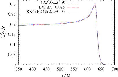
Figure 11: Comparison between the old and the new code. The plot shows the amplitude of the $(2,2)$ mode of the Regge-Wheeler-Zerilli as computed with the old code (at resolutions $\Delta r_{*}=0.5$ and $0.25$) based on the Lax-Wendroff scheme and with the new code (at resolution $\Delta r_{*}=0.5$). Other parameters of the runs are $\mu=0.001$, $R(0)=6.5$ and $c_{\rm cfl}=0.9$.

A direct comparison with the old code, Fig. 11, shows clearly that the numerical improvements lead to quantitative better results. The amplitude of $\Psi_{2\,2}$ is computed for two different resolution $\Delta r_{*}=0.5$ and $0.25$ using the old code based on the Lax-Wendroff scheme and with $\Delta r_{*}=0.5$ with the new scheme.

The differences are due only to the numerical scheme employed for the wave equation, since also the new radiation reaction has been used in the old code. As expected, the new numerical scheme shows a faster convergence and strongly suppresses the spurious oscillations coming from the boundaries; note in this respect the small “bumps” at $t\sim 400$ that are present only in the data computed with the old code.

To validate the physical results of the code at a more quantitative level we performed “standard” comparisons with the literature considering circular orbits and radial plunge, following the line of Nagar:2006xv .

Table 7: Gravitational wave (multipolar) energy flux $\dot{E}_{\ell m}/\mu^{2}$ of a particle on a circular orbit of radius $r_{0}=7.9456M$. Comparison between our results and those present in the literature. Our waveforms are extracted at $r_{*}=1000M$.

$\ell$ $m$	This work	Ref. Sopuerta:2005gz	Diff.[%]	Ref. Martel:2003jj	Diff.[%]	Ref. Poisson	Diff.[%]
2 1	8.1733$\times 10^{-7}$	8.1662$\times 10^{-7}$	0.086	8.1623$\times 10^{-7}$	0.134	8.1633$\times 10^{-7}$	0.122
2 2	1.7069$\times 10^{-4}$	1.7064$\times 10^{-4}$	0.029	1.7051$\times 10^{-4}$	0.105	1.7063$\times 10^{-4}$	0.035
3 1	2.1785$\times 10^{-9}$	2.1732$\times 10^{-9}$	0.242	2.1741$\times 10^{-9}$	0.200	2.1731$\times 10^{-9}$	0.246
3 2	2.5218$\times 10^{-7}$	2.5204$\times 10^{-7}$	0.057	2.5164$\times 10^{-7}$	0.217	2.5199$\times 10^{-7}$	0.077
3 3	2.5483$\times 10^{-5}$	2.5475$\times 10^{-5}$	0.031	2.5432$\times 10^{-5}$	0.201	2.5471$\times 10^{-5}$	0.047
4 1	8.3699$\times 10^{-13}$	8.4055$\times 10^{-13}$	0.423	8.3507$\times 10^{-13}$	0.230	8.3956$\times 10^{-13}$	0.306
4 2	2.5125$\times 10^{-9}$	2.5099$\times 10^{-9}$	0.103	2.4986$\times 10^{-9}$	0.556	2.5091$\times 10^{-9}$	0.135
4 3	5.7792$\times 10^{-8}$	5.7765$\times 10^{-8}$	0.046	5.7464$\times 10^{-8}$	0.571	5.7751$\times 10^{-8}$	0.071
4 4	4.7283$\times 10^{-6}$	4.7270$\times 10^{-6}$	0.027	4.7080$\times 10^{-6}$	0.430	4.7256$\times 10^{-6}$	0.056
5 1	1.2904$\times 10^{-15}$	1.2607$\times 10^{-15}$	2.357	1.2544$\times 10^{-15}$	2.871	1.2594$\times 10^{-15}$	2.462
5 2	2.7874$\times 10^{-12}$	2.7909$\times 10^{-12}$	0.126	2.7587$\times 10^{-12}$	1.040	2.7896$\times 10^{-12}$	0.080
5 3	1.0946$\times 10^{-9}$	1.0936$\times 10^{-9}$	0.095	1.0830$\times 10^{-9}$	1.074	1.0933$\times 10^{-9}$	0.122
5 4	1.2334$\times 10^{-8}$	1.2329$\times 10^{-8}$	0.038	1.2193$\times 10^{-8}$	1.154	1.2324$\times 10^{-8}$	0.078
5 5	9.4630$\times 10^{-7}$	9.4616$\times 10^{-7}$	0.014	9.3835$\times 10^{-7}$	0.847	9.4563$\times 10^{-7}$	0.071

The energy and angular momentum fluxes computed from the waveforms generated by a particle on a circular orbit of radius $r_{0}=7.9456M$ are displayed in Table 7 and Table 8. The numbers are compared with those present in the literature, showing very good agreement. The fractional differences are always well below the $1\%$ except for the multipole $(5,1)$ ($2\%$ in the energy flux) whose absolute value is the smallest. Notice that, differently from Ref. Nagar:2006xv , the accuracy is maintained also for high multipoles. We also computed multipoles for $\ell\geq 6$, although we did not report them here since corresponding data to compare with are not present in the literature.

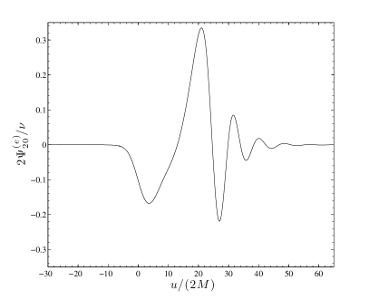
Figure 12: Waveform emitted by a particle plunging radially into the black hole (along the $z$-axis) from $r=10M$. The waveform is extracted at $r_{*}=1000M$.

For what concerns the radial infall, Fig. 12 displays the $\ell=2$, $m=0$ waveform generated by a particle plunging into the black hole radially along the $z$-axis. The particle has zero initial velocity and starts at $r=10M$. We specify conformally flat initial data according to the procedure described at the end of Sec. 4 of Nagar:2006xv . Note that $\Psi^{(\rm e)}_{20}$ has been multiplied by a factor 2 to facilitate the (very satisfactory) comparison with the top-right panel of Fig. 4 in Martel:2001yf and top-left panel of Fig. 6 in Lousto:1997wf .

Table 8: Gravitational wave (multipolar) angolar momentum flux $\dot{J}_{\ell m}/\mu^{2}$ of a particle on a circular orbit of radius $r_{0}=7.9456M$. Comparison between our results and those present in the literature. Our waveforms are extracted at $r_{*}=1000M$.

$\ell$ $m$	This work	Ref. Sopuerta:2005gz	Diff.[%]	Ref. Martel:2003jj	Diff.[%]	Ref. Poisson	Diff.[%]
2 1	1.8305$\times 10^{-5}$	1.8289$\times 10^{-5}$	0.090	1.8270$\times 10^{-5}$	0.194	1.8283$\times 10^{-5}$	0.122
2 2	3.8229$\times 10^{-3}$	3.8219$\times 10^{-3}$	0.027	3.8164$\times 10^{-3}$	0.171	3.8215$\times 10^{-3}$	0.037
3 1	4.8790$\times 10^{-8}$	4.8675$\times 10^{-8}$	0.237	4.8684$\times 10^{-8}$	0.219	4.8670$\times 10^{-8}$	0.247
3 2	5.6481$\times 10^{-6}$	5.6450$\times 10^{-6}$	0.055	5.6262$\times 10^{-6}$	0.389	5.6439$\times 10^{-6}$	0.075
3 3	5.7074$\times 10^{-4}$	5.7057$\times 10^{-4}$	0.030	5.6878$\times 10^{-4}$	0.345	5.7048$\times 10^{-4}$	0.046
4 1	1.8518$\times 10^{-11}$	1.8825$\times 10^{-11}$	1.633	1.8692$\times 10^{-11}$	0.933	1.8803$\times 10^{-11}$	1.517
4 2	5.6272$\times 10^{-8}$	5.6215$\times 10^{-8}$	0.102	5.5926$\times 10^{-8}$	0.619	5.6195$\times 10^{-8}$	0.138
4 3	1.2944$\times 10^{-6}$	1.2937$\times 10^{-6}$	0.052	1.2933$\times 10^{-6}$	0.083	1.2934$\times 10^{-6}$	0.075
4 4	1.0590$\times 10^{-4}$	1.0586$\times 10^{-4}$	0.037	1.0518$\times 10^{-4}$	0.684	1.0584$\times 10^{-4}$	0.056
5 1	2.8558$\times 10^{-14}$	2.8237$\times 10^{-14}$	1.138	2.8090$\times 10^{-14}$	1.667	2.8206$\times 10^{-14}$	1.249
5 2	6.2386$\times 10^{-11}$	6.2509$\times 10^{-11}$	0.197	6.1679$\times 10^{-11}$	1.146	6.2479$\times 10^{-11}$	0.149
5 3	2.4517$\times 10^{-8}$	2.4494$\times 10^{-8}$	0.093	2.4227$\times 10^{-8}$	1.196	2.4486$\times 10^{-8}$	0.125
5 4	2.7625$\times 10^{-7}$	2.7613$\times 10^{-7}$	0.042	2.7114$\times 10^{-7}$	1.883	2.7603$\times 10^{-7}$	0.078
5 5	2.1194$\times 10^{-5}$	2.1190$\times 10^{-5}$	0.020	2.0933$\times 10^{-5}$	1.248	2.1179$\times 10^{-5}$	0.072

An additional test involved the dependence of the results on the Gaussian ampitude $\sigma$. Focusing on $\mu=0.01$ and inspiral plunge simulations with $R(0)=6.5$ M, we experimented with the values $\sigma=\{0.05,0.1,0.5,1\}$ M using typical resolutions. The extreme value $\sigma=M$ (see discussion above) gave reliable waveforms, while spurious modulations due to the extended source were clearly evident for $\sigma>M$. Relative differences between $(2,2)$-waveforms, taking $\sigma=0.05$ M as reference value, were of the order of $\{10^{-2},\,10^{-3},\,10^{-4}\}$ in the amplitudes respectively for $\sigma=\{0.01,0.5,1\}$ M, and 1 order of magnitude less for the phase. For the $(8,8)$ multipole (worst case) they were $\{10^{-1},\,10^{-2},\,10^{-3}\}$ always for $\sigma=\{0.01,0.5,1\}$ M. The relative differences on the energy flux multipoles were of the order of $\{0.0002,\,0.007,\,0.03\}$ in the $(2,2)$ case and $\{0.005,\,0.2,\,0.9\}$ in the $(8,8)$ case. While $\sigma\geq 0.5$ M does not give satisfactory results, differences between $\sigma=0.05$ and $\sigma=0.1$ are quite small, giving the same results up to $0.5\%$ for the energy contribute. In the simulations of the paper we used $\sigma=0.04M$.

We also tested the use of the alternative source term (mathematically equivalent for a distributional source) given by Eq (23) of Nagar:2006xv . Consistently with the analysis of Ref. Nagar:2006xv (see their Fig. 5), for insplunge waveforms we found a relative difference smaller than $10^{-6}$ both in amplitude and phase in the $\ell=m=2$ mode.

We finally mention that in the case of long simulations (i.e., $\nu=10^{-3}$, $r_{0}=7M$) our boundary conditions are not fully satisfactory. In fact, in this case the waveforms might be (slightly) contaminated by small reflections from boundaries, especially for high multipoles. A solution to this problem is discussed in Lau:2005ti (and references therein), in which, basically, the free-data in the Sommerfeld condition (in our case they are set to zero) are specified as an integral convolution between a time-domain boundary kernel and the solution. The method provides an exact radiative outer boundary condition for the wave equations. We mention that an alternative approach is represented by solving the Regge-Wheeler-Zerilli equation on matched hyperboloidal foliations as described in Zenginoglu:2009ey (and references therein). The appealing feature is the fact that it has the double advantage to not need boundary conditions (no incoming modes) and to allow extraction exactly at null infinity.

Appendix B Partial losses during the plunge phase

Let us list here some useful numerical information related to the discussion of Sec. III.1; i.e, the energy and angular momentum emitted during the quasiuniversal part of the late-plunge, merger and ringdown. The pure numbers, up to multuipolar order $\ell=8$, are given in Table 9. The relative percentage (with respect to the “total” energy $E_{\rm TOT}$ and angular momentum $J_{\rm TOT}$) are given in the following Table 10. Note here that by total we indicate the sum over multipoles $(\ell,m)$, with $2\leq\ell\leq 8$ and $|m|\leq\ell$.

Table 9: Multipolar contributions to total energy and angular momentum emitted during the quasiuniversal part of the plunge phase, the merger and the ringdown.

Multipole		$\mu=0.001$		$\mu=0.0001$
$\ell$	$m$	$ME_{\ell m}/\mu^{2}$	$J_{\ell m}/\mu^{2}$	$ME_{\ell m}/\mu^{2}$	$J_{\ell m}/\mu^{2}$
2	0	9.739$\times 10^{-4}$	0	9.739$\times 10^{-4}$	0
	1	2.023 $\times 10^{-2}$	0.787 $\times 10^{-1}$	2.035 $\times 10^{-2}$	0.793 $\times 10^{-1}$
	2	2.733 $\times 10^{-1}$	2.150	2.769 $\times 10^{-1}$	2.179
3	0	3.320 $\times 10^{-5}$	0	3.330$\times 10^{-5}$	0
	1	0.540 $\times 10^{-3}$	1.196 $\times 10^{-3}$	0.543 $\times 10^{-3}$	1.201 $\times 10^{-3}$
	2	0.782 $\times 10^{-2}$	0.370 $\times 10^{-1}$	0.788 $\times 10^{-2}$	0.373 $\times 10^{-1}$
	3	0.929 $\times 10^{-1}$	0.678	0.941 $\times 10^{-1}$	0.687
4	0	1.518 $\times 10^{-6}$	0	1.523$\times 10^{-6}$	0
	1	2.226 $\times 10^{-5}$	0.333 $\times 10^{-4}$	2.234 $\times 10^{-5}$	0.334 $\times 10^{-4}$
	2	3.023 $\times 10^{-4}$	0.998 $\times 10^{-3}$	3.039 $\times 10^{-4}$	1.003 $\times 10^{-3}$
	3	0.330 $\times 10^{-2}$	1.657 $\times 10^{-2}$	0.332 $\times 10^{-2}$	1.674 $\times 10^{-2}$
	4	0.377 $\times 10^{-1}$	2.627 $\times 10^{-1}$	0.382 $\times 10^{-1}$	2.663 $\times 10^{-1}$
5	0	7.932 $\times 10^{-8}$	0	7.957 $\times 10^{-8}$	0
	1	1.042 $\times 10^{-6}$	1.205 $\times 10^{-6}$	1.046 $\times 10^{-6}$	1.209 $\times 10^{-6}$
	2	1.341 $\times 10^{-5}$	0.323 $\times 10^{-4}$	1.347 $\times 10^{-5}$	0.325 $\times 10^{-4}$
	3	1.659 $\times 10^{-4}$	0.642 $\times 10^{-3}$	1.670 $\times 10^{-4}$	0.647 $\times 10^{-3}$
	4	1.478 $\times 10^{-3}$	0.762 $\times 10^{-2}$	1.493 $\times 10^{-3}$	0.770 $\times 10^{-2}$
	5	1.683 $\times 10^{-2}$	1.129 $\times 10^{-1}$	1.705 $\times 10^{-2}$	1.145 $\times 10^{-1}$
6	0	4.182$\times 10^{-9}$	0	4.197$\times 10^{-9}$	0
	1	0.551 $\times 10^{-7}$	0.516 $\times 10^{-7}$	0.552 $\times 10^{-7}$	0.518 $\times 10^{-7}$
	2	0.673 $\times 10^{-6}$	1.312 $\times 10^{-6}$	0.676 $\times 10^{-6}$	1.317 $\times 10^{-6}$
	3	0.782 $\times 10^{-5}$	2.340 $\times 10^{-5}$	0.786 $\times 10^{-5}$	2.352 $\times 10^{-5}$
	4	0.904 $\times 10^{-4}$	0.379 $\times 10^{-3}$	0.910 $\times 10^{-4}$	0.382 $\times 10^{-3}$
	5	0.694 $\times 10^{-3}$	0.361 $\times 10^{-2}$	0.701 $\times 10^{-3}$	0.365 $\times 10^{-2}$
	6	0.799 $\times 10^{-2}$	0.518 $\times 10^{-1}$	0.809 $\times 10^{-2}$	0.526 $\times 10^{-1}$
7	0	2.416$\times 10^{-10}$	0	2.424 -10	0
	1	2.948 $\times 10^{-9}$	2.337 $\times 10^{-9}$	2.959 $\times 10^{-9}$	2.345 $\times 10^{-9}$
	2	0.360 $\times 10^{-7}$	0.586 $\times 10^{-7}$	0.362 $\times 10^{-7}$	0.588 $\times 10^{-7}$
	3	0.423 $\times 10^{-6}$	1.058 $\times 10^{-6}$	0.425 $\times 10^{-6}$	1.063 $\times 10^{-6}$
	4	0.448 $\times 10^{-5}$	1.516 $\times 10^{-5}$	0.451 $\times 10^{-5}$	1.526 $\times 10^{-5}$
	5	0.492 $\times 10^{-4}$	2.168 $\times 10^{-4}$	0.496 $\times 10^{-4}$	2.186 $\times 10^{-4}$
	6	0.337 $\times 10^{-3}$	1.760 $\times 10^{-3}$	0.341 $\times 10^{-3}$	1.781 $\times 10^{-3}$
	7	0.396 $\times 10^{-2}$	2.497 $\times 10^{-2}$	0.401 $\times 10^{-2}$	2.533 $\times 10^{-2}$
8	0	1.359 $\times 10^{-11}$	0	1.364 $\times 10^{-11}$	0
	1	1.699 $\times 10^{-10}$	1.163 $\times 10^{-10}$	1.704$\times 10^{-10}$	1.167$\times 10^{-10}$
	2	1.986 $\times 10^{-9}$	2.792 $\times 10^{-9}$	1.994 $\times 10^{-9}$	2.802 $\times 10^{-9}$
	3	2.303 $\times 10^{-8}$	0.491 $\times 10^{-7}$	2.313 $\times 10^{-8}$	0.493 $\times 10^{-7}$
	4	2.604 $\times 10^{-7}$	0.756 $\times 10^{-6}$	2.618 $\times 10^{-7}$	0.760 $\times 10^{-6}$
	5	2.539 $\times 10^{-6}$	0.931 $\times 10^{-5}$	2.558 $\times 10^{-6}$	0.938 $\times 10^{-5}$
	6	2.696 $\times 10^{-5}$	1.223 $\times 10^{-4}$	2.721 $\times 10^{-5}$	1.235 $\times 10^{-4}$
	7	1.680 $\times 10^{-4}$	0.878 $\times 10^{-3}$	1.701 $\times 10^{-4}$	0.890 $\times 10^{-3}$
	8	2.026 $\times 10^{-3}$	1.248 $\times 10^{-2}$	2.054 $\times 10^{-3}$	1.266 $\times 10^{-2}$

Table 10: Relative contribution of each multipole to the total energy and angular momentum emitted during the quasiuniversal part of the plunge phase, the merger and the ringdown.

Multipole		$\mu=0.001$		$\mu=0.0001$
$\ell$	$m$	$E_{\ell m}/E_{\rm TOT}[\%]$	$J_{\ell m}/J_{\rm TOT}[\%]$	$E_{\ell m}/E_{\rm TOT}$ $[\%]$	$J_{\ell m}/J_{\rm TOT}$ $[\%]$
2	0	0.2068	0	0.2050	0
	1	4.295	2.2868	4.268	2.2730
	2	58.03	62.45	58.07	62.46
3	0	7.0504 $\times 10^{-3}$	0	6.9844 $\times 10^{-3}$	0
	1	1.1475 $\times 10^{-1}$	0.3475 $\times 10^{-1}$	1.1378 $\times 10^{-1}$	0.3443 $\times 10^{-1}$
	2	1.6609	1.0735	1.6530	1.0689
	3	19.724	19.695	19.726	19.698
4	0	3.2237$\times 10^{-4}$	0	3.1947$\times 10^{-4}$	0
	1	0.4727 $\times 10^{-2}$	0.9683 $\times 10^{-3}$	0.4685 $\times 10^{-2}$	0.9586 $\times 10^{-3}$
	2	0.6419 $\times 10^{-1}$	0.2898 $\times 10^{-1}$	0.6372 $\times 10^{-1}$	0.2875 $\times 10^{-1}$
	3	0.6997	0.4814	0.6972	0.4799
	4	8.006	7.631	8.007	7.633
5	0	1.6843 $\times 10^{-5}$	0	1.6686$\times 10^{-5}$	0
	1	2.2133 $\times 10^{-4}$	0.3501 $\times 10^{-4}$	2.1936 $\times 10^{-4}$	0.3466 $\times 10^{-4}$
	2	2.8483 $\times 10^{-3}$	0.9389 $\times 10^{-3}$	2.8252 $\times 10^{-3}$	0.9305 $\times 10^{-3}$
	3	0.3523 $\times 10^{-1}$	0.1865 $\times 10^{-1}$	0.3501 $\times 10^{-1}$	0.1853 $\times 10^{-1}$
	4	0.3139	0.2213	0.3130	0.2208
	5	3.574	3.280	3.575	3.281
6	0	8.8792$\times 10^{-7}$	0	8.8013$\times 10^{-7}$	0
	1	1.1691 $\times 10^{-5}$	1.4994 $\times 10^{-6}$	1.1585 $\times 10^{-5}$	1.148428 $\times 10^{-6}$
	2	1.4293 $\times 10^{-4}$	0.3810 $\times 10^{-4}$	1.4172 $\times 10^{-4}$	0.3774 $\times 10^{-4}$
	3	1.6611 $\times 10^{-3}$	0.6796 $\times 10^{-3}$	1.6492 $\times 10^{-3}$	0.6742 $\times 10^{-3}$
	4	1.9185 $\times 10^{-2}$	1.1019 $\times 10^{-2}$	1.9085 $\times 10^{-2}$	1.0957 $\times 10^{-2}$
	5	1.4729 $\times 10^{-1}$	1.0489 $\times 10^{-1}$	1.4703 $\times 10^{-1}$	1.0470 $\times 10^{-1}$
	6	1.6963	1.5060	1.6970	1.5069
7	0	5.1297$\times 10^{-8}$	0	5.0836$\times 10^{-8}$	0
	1	0.6260 $\times 10^{-6}$	0.6787 $\times 10^{-7}$	0.6205 $\times 10^{-6}$	0.6720 $\times 10^{-7}$
	2	0.7651 $\times 10^{-5}$	1.7025 $\times 10^{-6}$	0.7585 $\times 10^{-5}$	1.6861 $\times 10^{-6}$
	3	0.8986 $\times 10^{-4}$	3.0728 $\times 10^{-5}$	0.8916 $\times 10^{-4}$	3.0458 $\times 10^{-5}$
	4	0.9508 $\times 10^{-3}$	0.4404 $\times 10^{-3}$	0.9450 $\times 10^{-3}$	0.4373 $\times 10^{-3}$
	5	1.0456 $\times 10^{-2}$	0.6296 $\times 10^{-2}$	1.0411 $\times 10^{-2}$	0.6266 $\times 10^{-2}$
	6	0.7152 $\times 10^{-1}$	0.5111 $\times 10^{-1}$	0.7145 $\times 10^{-1}$	0.5106 $\times 10^{-1}$
	7	0.8405	0.7254	0.8412	0.7260
8	0	2.8851$\times 10^{-9}$	0	2.8611$\times 10^{-9}$	0
	1	0.3608 $\times 10^{-7}$	0.3378 $\times 10^{-8}$	0.3574 $\times 10^{-7}$	0.3344 $\times 10^{-8}$
	2	0.4217 $\times 10^{-6}$	0.8109 $\times 10^{-7}$	0.4180 $\times 10^{-6}$	0.8031 $\times 10^{-7}$
	3	0.4889 $\times 10^{-5}$	1.4261 $\times 10^{-6}$	0.4850 $\times 10^{-5}$	1.4132 $\times 10^{-6}$
	4	0.5529 $\times 10^{-4}$	2.1963 $\times 10^{-5}$	0.5490 $\times 10^{-4}$	2.1788 $\times 10^{-5}$
	5	0.5391 $\times 10^{-3}$	2.7038 $\times 10^{-4}$	0.5364 $\times 10^{-3}$	2.6880 $\times 10^{-4}$
	6	0.5725 $\times 10^{-2}$	0.3553 $\times 10^{-2}$	0.5706 $\times 10^{-2}$	0.3539 $\times 10^{-2}$
	7	0.3566 $\times 10^{-1}$	0.2551 $\times 10^{-1}$	0.3566 $\times 10^{-1}$	0.2550 $\times 10^{-1}$
	8	0.4302	0.3624	0.4307	0.3628

References

- (1) F. Pretorius, Phys. Rev. Lett. 95, 121101 (2005) [arXiv:gr-qc/0507014].
- (2) M. Campanelli, C. O. Lousto, P. Marronetti and Y. Zlochower, Phys. Rev. Lett. 96, 111101 (2006) [arXiv:gr-qc/0511048].
- (3) J. G. Baker, J. Centrella, D. I. Choi, M. Koppitz and J. van Meter, Phys. Rev. Lett. 96, 111102 (2006) [arXiv:gr-qc/0511103].
- (4) M. Hannam, S. Husa, U. Sperhake, B. Bruegmann and J. A. Gonzalez, Phys. Rev. D 77, 044020 (2008) [arXiv:0706.1305 [gr-qc]].
- (5) M. Hannam, S. Husa, B. Bruegmann and A. Gopakumar, Phys. Rev. D 78, 104007 (2008) [arXiv:0712.3787 [gr-qc]].
- (6) U. Sperhake, V. Cardoso, F. Pretorius, E. Berti and J. A. Gonzalez, Phys. Rev. Lett. 101, 161101 (2008) [arXiv:0806.1738 [gr-qc]].
- (7) M. Campanelli, C. O. Lousto, H. Nakano and Y. Zlochower, Phys. Rev. D 79, 084010 (2009) [arXiv:0808.0713 [gr-qc]].
- (8) M. A. Scheel, M. Boyle, T. Chu, L. E. Kidder, K. D. Matthews and H. P. Pfeiffer, Phys. Rev. D 79, 024003 (2009) [arXiv:0810.1767 [gr-qc]].
- (9) T. Chu, H. P. Pfeiffer and M. A. Scheel, Phys. Rev. D 80, 124051 (2009) [arXiv:0909.1313 [gr-qc]].
- (10) P. Mosta, C. Palenzuela, L. Rezzolla, L. Lehner, S. Yoshida and D. Pollney, arXiv:0912.2330 [gr-qc].
- (11) D. Pollney, C. Reisswig, E. Schnetter, N. Dorband and P. Diener, arXiv:0910.3803 [gr-qc].
- (12) J. A. Gonzalez, U. Sperhake and B. Brugmann, Phys. Rev. D 79, 124006 (2009) [arXiv:0811.3952 [gr-qc]].
- (13) C. O. Lousto, H. Nakano, Y. Zlochower and M. Campanelli, arXiv:1001.2316 [gr-qc].
- (14) A. Buonanno and T. Damour, Phys. Rev. D 59, 084006 (1999) [arXiv:gr-qc/9811091].
- (15) A. Buonanno and T. Damour, Phys. Rev. D 62, 064015 (2000) [arXiv:gr-qc/0001013].
- (16) T. Damour, P. Jaranowski and G. Schaefer, Phys. Rev. D 62, 084011 (2000) [arXiv:gr-qc/0005034].
- (17) T. Damour, Phys. Rev. D 64, 124013 (2001) [arXiv:gr-qc/0103018].
- (18) A. Buonanno, Y. Chen and T. Damour, Phys. Rev. D 74, 104005 (2006) [arXiv:gr-qc/0508067].
- (19) T. Damour and A. Nagar, arXiv:0906.1769 [gr-qc].
- (20) A. Buonanno, Y. Pan, J. G. Baker, J. Centrella, B. J. Kelly, S. T. McWilliams and J. R. van Meter, Phys. Rev. D 76, 104049 (2007) [arXiv:0706.3732 [gr-qc]].
- (21) T. Damour and A. Nagar, Phys. Rev. D 77, 024043 (2008) [arXiv:0711.2628 [gr-qc]].
- (22) T. Damour, A. Nagar, E. N. Dorband, D. Pollney and L. Rezzolla, Phys. Rev. D 77, 084017 (2008) [arXiv:0712.3003 [gr-qc]].
- (23) T. Damour, A. Nagar, M. Hannam, S. Husa and B. Bruegmann, Phys. Rev. D 78, 044039 (2008) [arXiv:0803.3162 [gr-qc]].
- (24) M. Boyle, A. Buonanno, L. E. Kidder, A. H. Mroue, Y. Pan, H. P. Pfeiffer and M. A. Scheel, Phys. Rev. D 78, 104020 (2008) [arXiv:0804.4184 [gr-qc]].
- (25) A. Buonanno, Y. Pan, H. P. Pfeiffer, M. A. Scheel, L. T. Buchman and L. E. Kidder, Phys. Rev. D 79, 124028 (2009) [arXiv:0902.0790 [gr-qc]].
- (26) T. Damour and A. Nagar, Phys. Rev. D 79, 081503 (2009) [arXiv:0902.0136 [gr-qc]].
- (27) Y. Pan, A. Buonanno, L. T. Buchman, T. Chu, L. E. Kidder, H. P. Pfeiffer and M. A. Scheel, arXiv:0912.3466 [gr-qc].
- (28) E. Barausse and A. Buonanno, Phys. Rev. D 81, 084024 (2010), [arXiv:0912.3517 [gr-qc]].
- (29) http://lisa.nasa.gov
- (30) http://sci.esa.int/home/lisa/
- (31) A. Nagar, T. Damour and A. Tartaglia, Class. Quant. Grav. 24, S109 (2007) [arXiv:gr-qc/0612096].
- (32) T. Damour and A. Nagar, Phys. Rev. D 76, 064028 (2007) [arXiv:0705.2519 [gr-qc]].
- (33) T. Damour, B. R. Iyer and B. S. Sathyaprakash, Phys. Rev. D 57, 885 (1998) [arXiv:gr-qc/9708034].
- (34) T. Regge and J. A. Wheeler, Phys. Rev. 108, 1063 (1957).
- (35) F. J. Zerilli, Phys. Rev. Lett. 24, 737 (1970); Phys. Rev. D 2, 2141 (1970).
- (36) A. Nagar and L. Rezzolla, Class. Quant. Grav. 22, R167 (2005) [Erratum-ibid. 23, 4297 (2006)] [arXiv:gr-qc/0502064].
- (37) K. Martel and E. Poisson, Phys. Rev. D 71, 104003 (2005) [arXiv:gr-qc/0502028].
- (38) C. Cutler, E. Poisson, G. J. Sussman and L. S. Finn, Phys. Rev. D 47, 1511 (1993).
- (39) N. Yunes and E. Berti, Phys. Rev. D 77, 124006 (2008) [arXiv:0803.1853 [gr-qc]].
- (40) P. Pani, E. Berti, V. Cardoso, Y. Chen and R. Norte, Phys. Rev. D 81, 084011 (2010) [arXiv:1001.3031 [gr-qc]].
- (41) T. Damour, B. R. Iyer and A. Nagar, Phys. Rev. D 79, 064004 (2009) [arXiv:0811.2069 [gr-qc]].
- (42) L. E. Kidder, Phys. Rev. D 77, 044016 (2008) [arXiv:0710.0614 [gr-qc]].
- (43) L. Blanchet, G. Faye, B. R. Iyer and S. Sinha, arXiv:0802.1249 [gr-qc].
- (44) N. Yunes, A. Buonanno, S. A. Hughes, M. Coleman Miller and Y. Pan, Phys. Rev. Lett. 104, 091102 (2010) [arXiv:0909.4263 [gr-qc]].
- (45) S. Detweiler, Phys. Rev. D 77, 124026 (2008) [arXiv:0804.3529 [gr-qc]].
- (46) L. Barack and N. Sago, Phys. Rev. Lett. 102, 191101 (2009) [arXiv:0902.0573 [gr-qc]].
- (47) L. Barack and N. Sago, Phys. Rev. D 81, 084021 (2010) [arXiv:1002.2386 [gr-qc]].
- (48) L. Blanchet, S. Detweiler, A. Le Tiec and B. F. Whiting, Phys. Rev. D 81, 064004 (2010) [arXiv:0910.0207 [gr-qc]].
- (49) L. Blanchet, S. Detweiler, A. Le Tiec and B. F. Whiting, Phys. Rev. D 81, 084033 (2010) [arXiv:1002.0726 [gr-qc]].
- (50) T. Damour, Phys. Rev. D 81, 024017 (2010) arXiv:0910.5533 [gr-qc].
- (51) K. Glampedakis, S. A. Hughes and D. Kennefick, Phys. Rev. D 66, 064005 (2002) [arXiv:gr-qc/0205033].
- (52) S. A. Hughes, S. Drasco, E. E. Flanagan and J. Franklin, Phys. Rev. Lett. 94, 221101 (2005) [arXiv:gr-qc/0504015].
- (53) T. Damour, P. Jaranowski and G. Schafer, Phys. Lett. B 513, 147 (2001).
- (54) L. Blanchet, T. Damour and G. Esposito-Farese, Phys. Rev. D 69, 124007 (2004).
- (55) L. Blanchet, B. R. Iyer and B. Joguet, Phys. Rev. D 65, 064005 (2002) [Erratum-ibid. D 71, 129903 (2005)].
- (56) L. Blanchet and B. R. Iyer, Phys. Rev. D 71, 024004 (2005).
- (57) L. Blanchet, T. Damour, G. Esposito-Farese and B. R. Iyer, Phys. Rev. Lett. 93, 091101 (2004).
- (58) T. Tanaka, H. Tagoshi and M. Sasaki, Prog. Theor. Phys. 96, 1087 (1996) [arXiv:gr-qc/9701050].
- (59) J. N. Goldberg, J. MacFarlane, E. T. Newman,F. Rohrlich and E. C. G. Sudarsahn, J. Math. Phys. 8, 2155 (1967).
- (60) M. Davis, R. Ruffini, W. H. Press and R. H. Price, Phys. Rev. Lett. 27, 1466 (1971).
- (61) S. Chandrasekhar, “The mathematical theory of black holes,” Oxford, UK: Clarendon (1992) 646 p.
- (62) S. Chandrasekhar and S. Detweiler, Proc. Roy. Soc. Lond. A 344, 441 (1975).
- (63) E. W. Leaver, Proc. Roy. Soc. Lond. A 402, 285 (1985).
- (64) E. Berti, V. Cardoso and C. M. Will, Phys. Rev. D 73, 064030 (2006) [arXiv:gr-qc/0512160].
- (65) E. Berti, V. Cardoso and A. O. Starinets, Class. Quant. Grav. 26, 163001 (2009) [arXiv:0905.2975 [gr-qc]]. Note that Kerr black-hole frequencies (up to ) can be downloaded here http://wugrav.wustl.edu/people/BERTI/qnms.html
- (66) S. Hadar and B. Kol, arXiv:0911.3899 [gr-qc].
- (67) C. O. Lousto and R. H. Price, Phys. Rev. D 56, 6439 (1997) [arXiv:gr-qc/9705071].
- (68) K. Martel and E. Poisson, Phys. Rev. D 66, 084001 (2002) [arXiv:gr-qc/0107104].
- (69) C. F. Sopuerta and P. Laguna, Phys. Rev. D 73, 044028 (2006) [arXiv:gr-qc/0512028].
- (70) K. S. Thorne, Rev. Mod. Phys. 52, 299 (1980).
- (71) M. Ruiz, R. Takahashi, M. Alcubierre and D. Nunez, Gen. Rel. Grav. 40, 2467 (2008) [arXiv:0707.4654 [gr-qc]].
- (72) D. Pollney et al., Phys. Rev. D 76, 124002 (2007) [arXiv:0707.2559 [gr-qc]].
- (73) T. Damour and A. Gopakumar, Phys. Rev. D 73, 124006 (2006) [arXiv:gr-qc/0602117].
- (74) M. J. Fitchett, Mon. Not. Roy. Astron. Soc. 203, 1042 (1983).
- (75) M. J. Fitchett and S. Detweiler, Mon. Not. Roy. Astron. Soc. 211, 933 (1984).
- (76) M. Favata, S. A. Hughes and D. E. Holz, Astrophys. J. 607, L5 (2004) [arXiv:astro-ph/0402056].
- (77) C. F. Sopuerta, N. Yunes and P. Laguna, Phys. Rev. D 74, 124010 (2006) [Erratum-ibid. D 75, 069903 (2007 ERRAT,D78,049901.2008)] [arXiv:astro-ph/0608600].
- (78) L. Blanchet, M. S. S. Qusailah and C. M. Will, Astrophys. J. 635, 508 (2005) [arXiv:astro-ph/0507692].
- (79) A. Le Tiec, L. Blanchet and C. M. Will, Class. Quant. Grav. 27, 012001 (2010) [arXiv:0910.4594 [gr-qc]].
- (80) J. D. Schnittman and A. Buonanno, arXiv:astro-ph/0702641.
- (81) J. G. Baker, J. Centrella, D. I. Choi, M. Koppitz, J. R. van Meter and M. C. Miller, Astrophys. J. 653, L93 (2006) [arXiv:astro-ph/0603204].
- (82) J. A. Gonzalez, U. Sperhake, B. Bruegmann, M. Hannam and S. Husa, Phys. Rev. Lett. 98, 091101 (2007) [arXiv:gr-qc/0610154].
- (83) J. D. Schnittman et al., Phys. Rev. D 77, 044031 (2008) [arXiv:0707.0301 [gr-qc]].
- (84) T. Damour, A. Nagar and M. Trias, in preparation (2010).
- (85) T. Damour, B. R. Iyer and B. S. Sathyaprakash, Phys. Rev. D 62, 084036 (2000) [arXiv:gr-qc/0001023].
- (86) P. A. Sundararajan, G. Khanna and S. A. Hughes, arXiv:1003.0485 [gr-qc].
- (87) P. A. Sundararajan, G. Khanna and S. A. Hughes, Phys. Rev. D 76, 104005 (2007) [arXiv:gr-qc/0703028].
- (88) P. A. Sundararajan, Phys. Rev. D 77, 124050 (2008) [arXiv:0803.4482 [gr-qc]].
- (89) P. A. Sundararajan, G. Khanna, S. A. Hughes and S. Drasco, Phys. Rev. D 78, 024022 (2008) [arXiv:0803.0317 [gr-qc]].
- (90) G. Calabrese and C. Gundlach, Class. Quant. Grav. 23, S343 (2006) [arXiv:gr-qc/0509119].
- (91) K. Martel, Phys. Rev. D 69, 044025 (2004) [arXiv:gr-qc/0311017].
- (92) E. Poisson, Phys. Rev. D 52, 5719 (1995); Phys. Rev. D 55,7980 (1997).
- (93) S. R. Lau, J. Math. Phys. 46, 102503 (2005) [arXiv:gr-qc/0507140].
- (94) A. Zenginoglu, Class. Quant. Grav. 27, 045015 (2010) [arXiv:0911.2450 [gr-qc]].