Free Infinite Divisibility for Q-Gaussians

Abstract.

We prove that the $q$-Gaussian distribution is freely infinitely divisible for all $q\in[0,1]$.

1. Introduction

In this note we prove that the $q$-Gaussian distribution introduced by Bożejko and Speicher in [10] (see also the paper [9] of Bożejko, Kümmerer and Speicher) is freely infinitely divisible when $q\in[0,1]$.

We shall give a short outline for the context of this problem. In probability theory, the class of infinitely divisible distributions plays a crucial role, in the study of limit theorems, Lévy processes etc. So it was a remarkable discovery of Bercovici and Voiculescu [6] that there exists a corresponding class of freely infinitely divisible distributions in free probability. These distributions are typically quite different from the classically infinitely divisible ones; for example, many of them are compactly supported. Nevertheless, work of numerous authors culminating in the paper by [5] Bercovici and Pata showed that free ID distributions are in a precise bijection with the classical ones, this bijection moreover having numerous strong properties. For example, the semicircular law is the free analog of the normal distribution. From this bijection, one might get the intuition that, perhaps with very rare exceptions such as the Cauchy and Dirac distributions, some measures belong to the “classical” world and some to the “free” world. However, [4, Corollary 3.9] indicates that this intuition may be misleading: the normal distribution, perhaps the most important among the classical ones, is also freely infinitely divisible.

One approach towards understanding the relationship between the classical and free probability theories, and in particular the Bercovici-Pata bijection, have been attempts to construct an interpolation between these two theories. The oldest such construction, due to Bożejko and Speicher, is the construction of the $q$-Brownian motion. In particular, it provides a probabilistic interpretation for a (very classical) family of $q$-Gaussian distributions, which interpolate between the normal ($q=1$) and the semicircle ($q=0$) laws. Probably the best known description of the $q$-Gaussian distributions is in terms of their orthogonal polynomials $H_{n}(x|q)$ - called the $q$-Hermite polynomials - defined by the 3-term recurrence relation $xH_{n}(x|q)=H_{n+1}(x|q)+\frac{1-q^{n}}{1-q}H_{n-1}(x|q)$, with initial conditions $H_{0}(x|q)=1,$ $H_{1}(x|q)=x$. These polynomials have been studied for a long time: probably their first appearance under this guise occurred in L. J. Rogers’ 1893 paper [24]. Bożejko and Speicher construct their example of $q$-Brownian motion using creation-annihilation operators on a “twisted” Fock space: given a separable Hilbert space $H$ and $f\in H$, we let $c^{*}(f)$ be the left creation operator on the Fock space $\mathcal{F}(H)$ and $c(f)$ be its adjoint. The authors provide in [10] a scalar product $(\ \cdot\ |\ \cdot\ )_{q}$ on (a quotient space of) $\mathcal{F}(H)$ for which the so-called $q$-canonical commutation relation holds:

$$c(f)c^{*}(g)-qc^{*}(g)c(f)=(f|g)_{q}{\bf 1},\quad f,g\in H,$$

where 1 is the identity operator on $\mathcal{F}(H)$. It is a fundamental result that, when $(f|f)_{q}=1$, the distribution of the self-adjoint operator $c(f)+c^{*}(f)$ with respect to the vacuum state on $\mathcal{F}(H)$ is the (centered) $q$-Gaussian distribution of variance one, having the $q$-Hermite polynomials as orthogonal polynomials (see [9, Theorem 1.10]). In this case, as mentioned before, when $q=1$, $c(f)+c^{*}(f)$ is distributed according to the classical normal distribution $(2\pi)^{-1/2}\exp(t^{2}/2)dt$, and when $q=0$ according to the free central limit - the Wigner distribution with density $(2\pi)^{-1}\sqrt{4-t^{2}}\chi_{[-2,2]}(t)$. A formula for the density $f_{q}$ of the $q$-Gaussian distribution is provided in [19]: $f_{q}(x)=\pi^{-1}\sqrt{1-q}\sin\theta\prod_{n=1}^{\infty}(1-q)^{n}|1-q^{n}e^{2i\theta}|^{2},$ where $\cos\theta=\frac{x}{2}\sqrt{1-q}.$ The interested reader might want to note [19, Section III] that, up to a multiplicative constant depending only on $q$, $f_{q}$ is a theta function. For numerous details on properties and applications of $q$-Gaussian processes we refer to [9] and references therein.

As the construction described above suggests, $q$-Gaussians provide useful examples in operator algebras. The von Neumann algebras generated by families of $q$-Gaussians are shown to exhibit several interesting properties, and we shall list a few below; however, the structure of these algebras still remains largely mysterious. It is shown in [21] that algebras generated by such families when $f$ runs through $H$ and dim$(H)\geq 2$ are non-injective; the paper [23] proves that algebras generated by at least two $q$-Gaussians corresponding to orthogonal $f$s are always factors when $|q|<1$ (see also [15, 9, 26]), and in [25] Shlyakhtenko provides estimates for the non-microstates free entropy of $n$-tuples of such $q$-Gaussians, estimates which guarantee that the algebra they generate is solid in the sense of Ozawa whenever $q<\sqrt{2}-1$. Moreover, recently Bożejko [8] proved that in von Neumann algebras generated by two $q$-Gaussians, the Bessis-Moussa-Villani conjecture holds.

There are several strictly probabilistic approaches to $q$-Gaussians: we would like to mention the stochastic integration with respect to $q$-Brownian motion of Donati-Martin [14], the $q$-deformed cumulants, a $q$-convolution defined on a restricted class of probability measures and $q$-Poisson processes studied in [2] and a random matrix model provided in [18].

However, classical or free probability aspects of $q$-Gaussians have been less studied. In this paper, we show that all of these distributions, for $0\leq q\leq 1$, are freely infinitely divisible. This may be an indication that the class of freely infinitely divisible distributions, despite the Bercovici-Pata bijection, is quite different from the classical one, and is yet to be understood completely. The conjecture that $q$-Gaussian distributions are freely infinitely divisible when $q\in[0,1]$, formulated initially by the two last named authors and R. Speicher, was motivated among others by the recently proved free infinite divisibility of the classical Gaussian (corresponding to $q=1$). It has been shown in [4] that the Askey-Wimp-Kerov distributions with parameter $c\in[-1,0]$, and in particular the classical normal distribution (corresponding to $c=0)$ are $\boxplus$-infinitely divisible. This provided free infinite divisibility for distributions of several noncommutative Brownian motions (see for example [11, 12, 13]), interpolating between the classical central limit (the normal distribution) and the free central limit (the Wigner semicircle law). However, until now it remained a mystery whether this first (and most famous) such example of interpolation consists also of $\boxplus$-infinitely divisible distributions. Several numerical verifications performed by one of us seemed to indicate this is indeed the case. Here we shall give an answer to this question:

Theorem 1.

The $q$-Gaussian distribution $f_{q}(x)dx$ is freely infinitely divisible for all $q\in[0,1]$.

Our method to prove this result will be the same as in [4], namely we will construct an inverse to the Cauchy transform $G_{f_{q}}$ of the $q$-Gaussian defined on the whole lower half-plane. Then the Voiculescu transform $\phi_{f_{q}}(1/z)=G_{f_{q}}^{-1}(z)-(1/z)$ clearly has an extension to the whole complex upper half-plane $\mathbb{C}^{+}$. An application of the following theorem of Bercovici and Voiculescu from [6] yields the desired result:

Theorem 2.

A Borel probability measure $\mu$ on the real line is $\boxplus$-infinitely divisible if and only if its Voiculescu transform $\phi_{\mu}(z)$ extends to an analytic function $\phi_{\mu}\colon\mathbb{C}^{+}\to\mathbb{C}^{-}$.

The paper is organized as follows: in the second section, we introduce several notions and preliminary results used in our proof, and in the third section we give the proof of Theorem 1.

Acknowledgements. We would like to thank Roland Speicher for many useful discussions regarding this paper.

2. Preliminary results: the importance of an entire function

It is shown in the paper [27] of Pawel Szabłowski (see also [17]) that the density of the $q$-Gaussian distribution of mean zero and variance one, with respect to the Lebesgue measure is given by the formula

$$f_{q}(x)=\frac{\sqrt{1-q}}{2\pi}\sqrt{4-(1-q)x^{2}}\sum_{k=1}^{\infty}(-1)^{k-1}q^{\frac{k(k-1)}{2}}\mathcal{U}_{2k-2}\left(\frac{x\sqrt{1-q}}{2}\right),$$

for $|x|\leq 2/\sqrt{1-q}$, where $\mathcal{U}_{k}$ is the $k^{\rm th}$ Chebyshev polynomial of the second kind - defined by the relation $\mathcal{U}_{k}(\cos\theta)=\frac{\sin((k+1)\theta)}{\sin\theta}$. In our present paper we will consider this as being the definition of the $q$-Gaussian distribution.For simplicity of notation, we will re-normalize this density to being supported on $[-2,2]$, by replacing $x$ with $x/\sqrt{1-q}:$

$$f_{q}(x)=\frac{1}{2\pi}\sqrt{4-x^{2}}\sum_{k=1}^{\infty}(-1)^{k-1}q^{\frac{k(k-1)}{2}}\mathcal{U}_{2k-2}\left(\frac{x}{2}\right),\quad-2\leq x\leq 2.$$

Recall that the Cauchy (or Cauchy-Stieltjes) transform of a Borel probability measure $\mu$ on $\mathbb{R}$ is by definition

$$G_{\mu}(z)=\int_{\mathbb{R}}\frac{1}{z-x}\,d\mu(x),\quad z\in\mathbb{C}\setminus\mathbb{R}.$$

This function maps the upper half-plane $\mathbb{C}^{+}$ into the lower half-plane $\mathbb{C}^{-}$, satisfies $G_{\mu}(\overline{z})=\overline{G_{\mu}(z)}$, and extends analytically through the complement of the support of $\mu$. Also, of some importance for us will be the map $F_{\mu}(z)=\frac{1}{G_{\mu}(z)}$. This function satisfies the inequality $\Im F_{\mu}(z)>\Im z$, $z\in\mathbb{C}^{+}$, whenever $\mu$ is not a point mass. For more details we refer the reader to the third chapter of [1, Chapter III].

Integrating $(z-x)^{-1}f_{q}(x)$ with respect to the Lebesgue measure on $[-2,2]$, we obtain for any $z\in\mathbb{C}^{+}$ that

$$G_{f_{q}}(z) = \int_{-2}^{2}\frac{1}{z-x}f_{q}(x)dx$$

$$= \sum_{k=1}^{\infty}(-1)^{k-1}q^{\frac{k(k-1)}{2}}\left(\frac{1}{2\pi}\int_{-2}^{2}\frac{1}{z-x}\mathcal{U}_{2k-2}\left(\frac{x}{2}\right)\sqrt{4-x^{2}}\,dx\right)$$

$$= \sum_{k=1}^{\infty}(-1)^{k-1}q^{\frac{k(k-1)}{2}}G_{s}(z)^{2k-1}$$

$$= \sum_{k=0}^{\infty}(-1)^{k}q^{\frac{k(k+1)}{2}}G_{s}(z)^{2k+1},$$

where $G_{s}$ is the Cauchy transform of the semicircular law:

$$G_{s}(z)=\frac{1}{2\pi}\int_{-2}^{2}\frac{1}{z-x}\sqrt{4-x^{2}}\,dx=\frac{z-\sqrt{z^{2}-4}}{2},\quad z\in\mathbb{C}^{+}.$$

This function has an analytic extension to the lower half-plane $\mathbb{C}^{-}$ through the interval $(-2,2)$ that does not coincide with $(2\pi)^{-1}\int_{-2}^{2}(z-x)^{-1}\sqrt{4-x^{2}}dx$ when $z\in\mathbb{C}^{-}$: when we consider the same branch of the square root as above, it is of the form $G_{s}(z)=\frac{z+\sqrt{z^{2}-4}}{2}$ (meaning, the asymptotics of this extension at $-i\infty$ is $O(z)$). An analysis of these two formulas guarantee us that $G_{s}$ maps $\mathbb{C}^{+}\cup(-2,2)\cup\mathbb{C}^{-}$ bijectively onto $\mathbb{C}^{-}$ by mapping $\mathbb{C}^{+}$ into the lower half of the unit disc $\mathbb{D}$ (the piece of $\partial G_{s}(\mathbb{C}^{+})$ that forms the interval $[-1,1]$ is $G_{s}([-\infty,-2]\cup[2,+\infty])$, with the two infinities identified and $G_{s}(\infty)=0$), while $G_{s}(\mathbb{C}^{-})$ is the complement of $\overline{G_{s}(\mathbb{C}^{+})}$ in $\mathbb{C}^{-}$. In addition, $G_{s}(i\mathbb{R}_{+})=i[-1,0)$, $G_{s}(i\mathbb{R}_{-})=i(-\infty,-1]$ and, when discarding the $i$, $G_{s}$ is monotonic increasing on the imaginary axis. These simple observations will be essential in our proof.

Now observe that the above remarks translate into $G_{f_{q}}=g_{q}\circ G_{s}$, where

(1) $$g_{q}(w)=\sum_{k=0}^{\infty}(-1)^{k}q^{\frac{k(k+1)}{2}}w^{2k+1},\quad w\in\mathbb{C},$$

is an entire function for any $q\in[0,1)$ (in fact for any $|q|<1$).  (The reader will note that in terms of basic hypergeometric functions $g_{q}$ can be written as $g_{q}(w)=w\cdot{}_{1}\phi_{0}(q^{\frac{1}{2}}|q^{\frac{1}{2}},(iq^{\frac{1}{2}}w)^{2})$; however, we shall not use this fact directly in our proof.) We list below a few properties of $g_{q}$ which will be used in our proof:

1. $\lim_{q\to 0}g_{q}(w)=w,w\in\mathbb{C}$, and the limit is uniform on compacts in $\mathbb{C}$;

2. $\lim_{q\to 1}g_{q}(w)=\frac{w}{w^{2}+1},w\neq\pm i$;

3. $g_{q}(-\overline{w})=-\overline{g_{q}(w)};$

4. $g_{q}(\overline{w})=\overline{g_{q}(w)}$ - in particular $g_{q}(\mathbb{R})\subseteq\mathbb{R}$;

5. $g_{q}(ic)=i\sum_{k=0}^{\infty}q^{\frac{k(k+1)}{2}}c^{2k+1}$ for any real $c$, so that $g_{q}(i(-\infty,0])=i(-\infty,0]$, $g_{q}(i[0,+\infty))=i[0,+\infty)$, with $g_{q}(i(\pm\infty))=i(\pm\infty)$, $g_{q}(0)=0$, and $g_{q}$ is monotonic on the imaginary axis (in the same sense as $G_{s}$ is);

6. $g_{q}^{\prime}(0)=1$.

The limits in items (1), (2) above being uniform on the corresponding compact subsets, we can conclude that, given $M>0$, for $q>0$ sufficiently small, depending on $M$, we have that $g_{q}$ is injective on the ball of radius $M$ centered at the origin, In addition, Equation (4) below guarantees that $g_{q}$ has no limit at infinity along the real axis; items (3) and (4) above together with this remark guarantee that $g_{q}^{\prime}$ will have at least two zeros on the real line, symmetric with respect to zero, if $q>0$.

It is time for stating a few results to be used in our proof:

Theorem 3.

A necessary and sufficient condition that

$$f(z)=\sum_{n=0}^{\infty}a_{n}z^{n}$$

should be an entire function of order $\varrho$ is that

$$\liminf_{n\to\infty}\left(\frac{-\log|a_{n}|}{n\log n}\right)=\frac{1}{\varrho}.$$

(This is [16, Theorem 4.12.1].) Thus, for our $g_{q}$, we can take $\infty=\lim_{n\to\infty}\left(\frac{-n(n+1)\log q}{2(2n+1)\log(2n+1)}\right)=\frac{1}{\varrho}$ to conclude that the order $\varrho$ of $g_{q}$ is zero.

Let us also give the Denjoy-Carleman-Ahlfors Theorem:

Theorem 4.

1. An entire function of order $\varrho$ has at most $2\varrho$ finite asymptotic values.

2. For an entire function of order $\varrho$ the sets $\{z\in\mathbb{C}\colon|f(z)|>c\}$, $c\geq 0$, have at most $\max\{2\varrho,1\}$ components.

In particular, the function $g_{q}$ has no finite asymptotic value and the sets $\{z:|g_{q}(z)|>c\}$ have exactly one connected component.

Two very famous theorems, available in any complex analysis text:

Theorem 5.

Any nonconstant analytic function is open, i.e. maps open sets into open sets. In particular, if $f$ is analytic and nonconstant, $\partial f(D)\subseteq f(\partial D)$ for a given open $D$.

Theorem 6.

Assume that $f,g$ are analytic on the simply connected domain $D$, and $\gamma$ is a rectifiable simple closed curve in $D$. If $|f(z)+g(z)|<|f(z)|+|g(z)|$ for all $z$ in the range of $\gamma$, then $f$ and $g$ have the same number of zeros in the subdomain delimited by $\gamma$ inside $D$.

The first is the open mapping theorem, the second a weakened version of Rouché’s theorem - the variation of argument.

Finally, let us denote following [3], page 81,

(2) $$\theta_{1}(z)=-iq^{1/4}\sum_{n=-\infty}^{\infty}(-1)^{n}q^{n^{2}+n}e^{i(2n+1)z}=-iqG\prod_{n=1}^{\infty}(1-q^{2n-2}e^{-2iz})(1-q^{2n}e^{2iz})e^{iz}.$$

We do the obvious substitution $z=-i\log w$ to get the new function

(3) $$\Theta(w) = -iq^{1/4}\sum_{n=-\infty}^{\infty}(-1)^{n}q^{n^{2}+n}w^{2n+1}$$

$$= -iq^{1/4}\left(g_{q^{2}}(w)-g_{q^{2}}\left(\frac{1}{w}\right)\right).$$

The letter $G$ in formula (2) denotes a complex constant, not a Cauchy transform; we preserve this notation just in order to follow [3]. Second, while $\theta_{1}$ is entire (and one can see that from either of the two formulas - the infinite product or the bi-infinite sum - since, for example, $|(e^{iz})^{(2\pm\frac{1}{n})}|<|q^{-|n|+1}|$ for $|n|$ large enough), this is not the case, of course, with $\Theta$. (We will generally ignore reparametrizations of $q$, since they won’t be important.) This new function is not analytic anymore at zero. Here it is important however to observe the product formula for our function: the above provides us with

(4) $$\Theta(w)=-iq^{1/4}\left(g_{q^{2}}(w)-g_{q^{2}}\left(\frac{1}{w}\right)\right)=-iqG\prod_{n=1}^{\infty}(1-q^{2n-2}w^{-2})(1-q^{2n}w^{2})w.$$

Thus, all zeros of $\Theta:w\mapsto-iq^{1/4}\left(g_{q^{2}}(w)-g_{q^{2}}\left(\frac{1}{w}\right)\right)$ are real (namely $w=\pm q^{n-1}$ and $w=\pm q^{-n}$, $n\in\mathbb{N}$; $w=0$ is not a zero of this function, since zero is an accumulation point of other zeros).

Let us give a few trivial lemmas:

Lemma 7.

Assume that an entire analytic function $h$ has order zero. Then the preimage $h^{-1}(l)$ of any piecewise smooth curve $l$ with both ends at infinity has all its ends tend to infinity and for any component $\gamma$ of $h^{-1}(l)$, we have $h(\gamma)=l$.

Proof.

It is clear from Theorem 5 and the definition of an entire function that the preimage of any curve with both ends at infinity cannot have an end in the complex plane.

On the other hand, by the Denjoy-Carleman-Ahlfors Theorem (Theorem 4), we know that there is no path $\gamma$ going to infinity so that the limit of $h$ along $\gamma$ is finite. If we assume that there is a branch $\gamma$ of $h^{-1}(l)$ so that $h(\gamma)\neq l$, then there exists a complex number $c\in l$ which is an asymptotic value for $h$ at infinity, contradicting Theorem 4. ∎

Lemma 8.

1. If $\gamma$ is the boundary of a simply connected domain $D$ in $\mathbb{C}$, $\gamma$ has both ends at infinity, and $h(\gamma)=\mathbb{R}$, then either $h(D)$ is one of the domains $\mathbb{C}^{+},\mathbb{C}^{-},$ or $\overline{h(D)}=\mathbb{C}$.

2. If $h(\partial D)$ is a half-line $s$ in $\mathbb{C}$, then ${h(D)}\supseteq\mathbb{C}\setminus s$.

Proof.

As seen in Theorem 5, $\partial h(D)\subseteq h(\gamma)=\mathbb{R}$. It is clear that if $h(D)$ is not a half-plane, then its closure must be all of $\mathbb{C}$. This proves (a). The proof of (b) is identical: $\partial h(D)\subseteq h(\partial D)=s$, so ${h(D)}\supseteq\mathbb{C}\setminus s$. ∎

Lemma 9.

With the notations from the previous lemma, if $\gamma$ is a rectifiable path, $h(D)=\mathbb{C}^{+}$, and $h$ is injective on $\gamma$, then $h$ maps $D$ conformally onto $\mathbb{C}^{+}$.

Proof.

This lemma is a direct consequence of [22], Chapters 1 and 2. ∎

3. Proof of free infinite divisibility for $f_{q}(x)dx$

We are now ready to prove the main result. For the comfort of the reader, we restate our main Theorem 1 below.

Theorem 1.

The $q$-Gaussian distribution $f_{q}(x)dx$ is freely infinitely divisible for all $q\in[0,1]$.

Proof.

In our proof, we will follow the outline described in the introduction. Namely, we will find a domain $X_{q}$ in the lower half-plane containing the lower half of the unit disc $\mathbb{D}$ with the property that $g_{q}(X_{q})=\mathbb{C}^{-}$ and $g_{q}$ is injective on $X_{q}$. Since we have shown that $G_{s}$ maps $\mathbb{C}^{+}\cup\mathbb{R}$ injectively into the closure of the lower half of the unit disc and (when considering the correct extension through $(-2,2)$) $\mathbb{C}^{-}$ injectively into $\mathbb{C}^{-}\setminus\overline{\mathbb{D}}$, it will follow that $G_{f_{q}}^{-1}=G_{s}^{-1}\circ g_{q}^{-1}$ extends to $\mathbb{C}^{-}$. Thus,

$$F_{f_{q}}(\cdot)=\frac{1}{g_{q}(G_{s}(\cdot))}\colon G^{-1}_{s}(X_{q})\mapsto\mathbb{C}^{+}$$

is a bijective correspondence. (The reader should keep in mind that $G_{s}^{-1}$ is the inverse of the extension of $G_{s}|_{\mathbb{C}^{+}}$ through $(-2,2)$, so $G^{-1}_{s}(X_{q})\supset\mathbb{C}^{+}$.) Since $X_{q}$ is included in the lower half-plane, the choice of the extension of $G_{s}$ guarantee that $G^{-1}_{s}(X_{q})\cap\mathbb{R}=(-2,2)$. This implies the existence of $\phi_{f_{q}}(z)=F_{f_{q}}^{-1}(z)-z$ for all $z\in\mathbb{C}^{+}$. Recalling now that $\Im F_{f_{q}}(w)>\Im w$ for all $w\in\mathbb{C}^{+}$, we obtain that $\Im F_{f_{q}}(w)>\Im w$ for all $w\in G^{-1}_{s}(X_{q})$, and hence $\Im\phi_{f_{q}}(z)=\Im F_{f_{q}}^{-1}(z)-\Im z<0$ for all $z\in\mathbb{C}^{+}$. An application of Theorem 2 yields the desired conclusion.

First, remark that, since $g_{q}^{\prime}(0)=1$, for any fixed $q\in(0,1)$ there exist two constants $K_{q},M_{q}>0$ so that $g_{q}$ is injective on $K_{q}\mathbb{D}$ and $g_{q}(K_{q}\mathbb{D})\supset M_{q}\mathbb{D}$.

Next, we shall construct the domain $X_{q}$ described in the first paragraph of the proof. Since $g_{q}(z)=-g_{q}(-z)$ and $g_{q}(\overline{z})=\overline{g_{q}(z)}$, $z\in\mathbb{C}$, it will clearly be enough to find the right side of $X_{q}$, as $X_{q}$ must be symmetric with respect to the imaginary axis. As suggested by the last lemma, we shall first find a continuous simple path inside $\overline{\mathbb{C}^{-}}$ whose image via $g_{q}$ is the real line. We observe in addition that, due to the symmetry noted in items (3), (4) and (5) in the above list of properties of $g_{q}$, it will be enough to determine the right half of such a path (see Figure 1.)

We start our path from zero. Let us now “walk” along the real axis, in the positive direction (by item (3) above, it is enough if we cover the right half) until we encounter a zero of $g_{q}^{\prime}$, call it $d_{q}$. Clearly, $g_{q}([0,d_{q}])=[0,g_{q}(d_{q})]$ is a bijective identification. Around $d_{q}$, $g_{q}$ will be an $n$-to-one cover (where $n$ is the order of the zero of $g_{q}(\cdot)-g_{q}(d_{q})$), and we will choose the path “first to the right” which continues $g_{q}^{-1}([0,g_{q}(d_{q})])$ beyond $d_{q}$, to $g_{q}^{-1}([0,+\infty))$. Observe that this path escapes now in the lower half-plane and, since $g_{q}(\mathbb{R})\subseteq\mathbb{R}$, it remains in the lower half-plane. Now whenever we meet another such critical point for $g_{q}$ on this path $g_{q}^{-1}([0,+\infty))$, we turn again “first to the right”, so that immediately to the right of this branch of $g_{q}^{-1}([0,+\infty))$ of ours, $g_{q}$ is injective. Call this branch - which is a rectifiable, piecewise analytic path - $\gamma_{q}$. Observe moreover that, by item (5), $\gamma_{q}$ is confined to the lower right quadrant of the complex plane (it cannot cut the imaginary axis, as the imaginary axis is mapped into itself).

Apriori it is not clear whether this branch of $g_{q}^{-1}([0,+\infty))$ is in fact existing, i.e. $g_{q}(\gamma_{q})=[0,+\infty)$. However, as we have seen above, $g_{q}$ has order zero, so by Lemma 7 (the application of the Denjoy-Carleman-Ahlfors Theorem), $g_{q}$ can have no finite asymptotic values at infinity, so indeed $\gamma_{q}$ as above (i.e. $g_{q}(\gamma_{q})=[0,+\infty)$) exists. Thus $\gamma_{q}\cup(-\overline{\gamma_{q}})$ (here $\overline{\gamma}$ means complex conjugate, not closure) forms the boundary of a unique simply connected domain $X_{q}\subseteq\mathbb{C}^{-}$ which contains the lower half of the imaginary axis and has a piecewise analytic, everywhere continuous, boundary. Clearly the lower half of the unit disc is included in $X_{q}$. Indeed, if $\gamma_{q}\cap\mathbb{D}\neq\varnothing$, then there exists $z_{0}\in\mathbb{C}^{+}$ so that $G_{s}(z_{0})\in\gamma_{q}\cap\mathbb{D}$, and thus $G_{f_{q}}(z_{0})=g_{q}(G_{s}(z_{0}))\in\mathbb{R}$, an obvious contradiction.

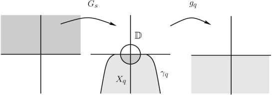
Figure 1. The curve $\gamma_{q}$ is mapped by $g_{q}$ onto the real line. The darker shadings correspond to each other via $G_{s}$, while $g_{q}$ maps the entire shaded area (dark and light) onto the lower half-plane.

Fix now $q\in(0,1)$. It is trivial that $g_{q}$ has a unique inverse, call it $\Phi$, defined around zero (more precise, at least on $M_{q}\mathbb{D}$), which fixes zero. We would like to extend this inverse to the whole lower half-plane; then it would easily follow that $\Phi(\mathbb{C}^{-})=X_{q}$. The lack of finite asymptotic values for $g_{q}$ guarantees that the only impediment to such an analytic extension would be a finite critical value of $g_{q}$. Thus, assume towards contradiction that there exists a $c\in X_{q}$ (for precision, assume $\Re c>0$) so that $g_{q}^{\prime}(c)=0$. Without loss of generality we may assume that $g_{q}(c)\in\mathbb{C}^{-}$ and $g_{q}(c)$ is the point closest to the origin in the lower half-plane to which $\Phi$ does not extend analytically. We consider a half-line $r$ starting at $g_{q}(c)$ and going to infinity inside $\mathbb{C}^{-}\cap i\mathbb{C}^{-}$ without cutting $g_{q}(c)\mathbb{D}$ and so that no $z\in r\setminus\{g_{q}(c)\}$ is a critical value for $g_{q}$ (possible since the set of critical values of $g_{q}$ is at most countable). By the same Lemma 7, we conclude that $r$ has a preimage $p_{q}$ via $g_{q}$ inside $X_{q}$, right of the imaginary axis, with both ends at infinity, which determines a domain $D\subset X_{q}$ that does not contain $i(-\infty,0)$ and having boundary $\partial D=p_{q}$. The choice for $p_{q}$ is made so that there is no other preimage in $X_{q}\setminus D$ of $r$ which is in the same connected component of $g_{q}^{-1}(r)$ as $p_{q}$.

For the sake of clarity, we group most of the rest of the proof in the following lemma. The reader will probably find Figure 2 helpful in following it.

Lemma 10.

1. There exists a point $b\in D$, $|b|>1$, so that $g_{q}(b)=0$.

2. For any $m>|c|+|g_{q}(c)|+1+|b|$, there exists $M\geq m$ and a path $\varpi$ in $\overline{D}$ uniting the two points of $p_{q}\cap g_{q}^{-1}(\partial(M\mathbb{D}))$ so that $g_{q}(\varpi)\cap m\mathbb{D}=\varnothing$.

3. Let $\Pi_{m}$ be the path obtained by concatenating $\varpi$, the bounded part(s) of $p_{q}\setminus(\varpi\cup\mathbb{D})$ and, if existing, the segments $\partial\mathbb{D}\cap D$. Then $\Pi_{m}$ is a closed curve containing $b$ inside it and there exists $m>0$ so that $\{g_{q}(1/w)\colon w\in\Pi_{m}\}\subset\mathbb{C}^{+}$ and $g_{q}(\Pi_{m})\cap\{g_{q}(1/w)\colon w\in\Pi_{m}\}=\varnothing$.

4. In particular, $w\mapsto g_{q}(w)$ and $w\mapsto g_{q}(w)-g_{q}(1/w)$ have the same number of zeros in the simply connected domain determined by the simple closed curve $\Pi_{m}$.

Proof.

Clearly, Lemma 8 guarantees that $g_{q}(D)\supseteq\mathbb{C}\setminus r$, which contains zero. Thus, there exists a point $b\in D$ so that $g_{q}(b)=0$. Moreover, let us recall that $G_{f_{q}}=g_{q}\circ G_{s}$ is the Cauchy transform of a probability measure, and, as such, it maps the upper half-plane into the lower one. Thus, as $G_{s}(\mathbb{C}^{+}\cup[-2,2])=\overline{\mathbb{D}}\cap\mathbb{C}^{-}$, it follows that $g_{q}(w)\neq 0$ for any $w\in\overline{\mathbb{D}}\cap\mathbb{C}^{-}$, so $b\in\mathbb{C}^{-}\setminus\overline{\mathbb{D}},$ so in particular $|b|>1$. This proves (1).

To prove (2), recall that by Theorem 4 the set $\{z\in\mathbb{C}\colon|g_{q}(z)|>m\}$ is connected for any $m\geq 0$ and in particular for $m$ as in the statement of the lemma. Also, from the construction of $r$ and $p_{q}$, it is clear that $p_{q}\cap g_{q}^{-1}(\partial(M\mathbb{D}))$ contains exactly two points for any $M\geq m$. Assume now towards contradiction that there is no path uniting those two points inside the set $D\setminus g^{-1}_{q}(m{\mathbb{D}})$, and in particular, of course, in $D\setminus g^{-1}_{q}(m\overline{\mathbb{D}})$. Thus the open set $g^{-1}_{q}(m{\mathbb{D}})\cap D$ must contain an unbounded smooth path. Choose such a path, and call it $\Gamma$. Choose $0<T=1+2\inf\{|z|\colon z\in\Gamma\}$ (so that $\Gamma\cap T\mathbb{D}\neq\varnothing$) and let $M>2\max\{|g_{q}(z)|\colon|z|\leq T\}+m$. Since $g_{q}(\overline{z})=\overline{g_{q}(z)}$, it follows that $\{z\in\mathbb{C}\colon|g_{q}(z)|>M\}$ does not intersect the set $T\mathbb{D}\cup\Gamma\cup\overline{\Gamma}$ (here again $\overline{\Gamma}$ denotes complex conjugate, not closure). But this set disconnects $\mathbb{C}$: for example, the set $p_{q}\cap\{z\in\mathbb{C}\colon|g_{q}(z)|>M\}$ contains two nonempty connected components separated by $T\mathbb{D}\cup\Gamma\cup\overline{\Gamma}$. This contradicts Theorem 4. Thus a path $\varpi=\varpi_{m}$ as described in our lemma must exist.

The fact that $\Pi_{m}$ exists and surrounds $b$ exactly once is a trivial consequence of (1), (2) and the entireness of $g_{q}$. Moreover, from $\Pi_{m}$’s construction, the set $\{1/w\colon w\in\Pi_{m}\}\subset\mathbb{C}^{+}\cap\overline{\mathbb{D}}$. Thus, as noted in the proofs of (1) and (2), $\{g_{q}(1/w)\colon w\in\Pi_{m}\}\subset g_{q}(\mathbb{D}\cap\mathbb{C}^{+})\subset\mathbb{C}^{+}$ (recall that $g_{q}(\overline{z})=\overline{g_{q}(z)}$) is a bounded set for any $m$ (one can choose the bound $\max g_{q}(\overline{\mathbb{D}})$, which is obviously independent of $m$ and depends only on $q$). To finish the proof of (3) we only need to argue that for $m$ large enough, the set $g_{q}(\Pi_{m})$ does not intersect $\mathbb{C}^{+}\cap(\max g_{q}(\overline{\mathbb{D}})\mathbb{D})$. Indeed, if we have a point $z\in p_{q}$, then $g_{q}(z)\in r\subset\mathbb{C}^{-}$, while if $z\in\partial\mathbb{D}\cap\mathbb{C}^{-}$, then again $g_{q}(z)\in\mathbb{C}^{-}.$ We only need to show that for $m$ large enough $\varpi=\varpi_{m}$ is mapped in the complement of $\max g_{q}(\overline{\mathbb{D}})\mathbb{D}$. However, this follows from part (2) by simply choosing $m\geq\max g_{q}(\overline{\mathbb{D}})$. This proves (3).

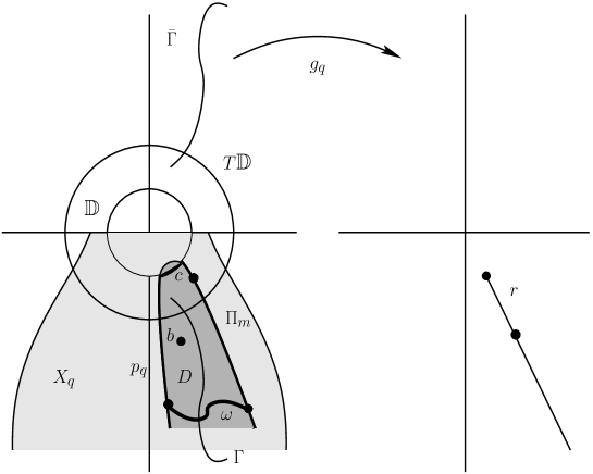
Figure 2. The region shaded in dark grey is mapped by $g_{q}$ surjectively onto $\mathbb{C}\setminus r$.

In order to prove (4), we will apply Theorem 6 to $f(z)=-g_{q}(z)+g_{q}(1/z)$ and $g(z)=g_{q}(z)$. The relation $|g_{q}(z)+(-g_{q}(z)+g_{q}(1/z))|<|g_{q}(z)-g_{q}(1/z)|+|g_{q}(z)|$ is equivalent to $\left|\frac{g_{q}(1/z)}{g_{q}(z)}\right|<\left|\frac{g_{q}(z)-g_{q}(1/z)}{g_{q}(z)}\right|+1=\left|1-\frac{g_{q}(1/z)}{g_{q}(z)}\right|+1,$ for $z\in\Pi_{m}$. Consider two cases: first, if $z\in\varpi$, then $|g_{q}(z)|>m>|g_{q}(1/z)|$, so that $\left|\frac{g_{q}(1/z)}{g_{q}(z)}\right|-1<0<\left|1-\frac{g_{q}(1/z)}{g_{q}(z)}\right|$. Second case, if $z\in\Pi_{m}\setminus\varpi$, then $g_{q}(z)\in\mathbb{C}^{-}$ and $g_{q}(1/z)\in\mathbb{C}^{+}$. Thus, $g_{q}(z)$ and $g_{q}(1/z)$ cannot be positive multiples of each other, i.e. $\frac{g_{q}(1/z)}{g_{q}(z)}\not\in[0,+\infty)$. Generally, for the relation $|a|-1=|a-1|$ to hold it is necessary that $a\geq 1$. Applying this observation to $a=\frac{g_{q}(1/z)}{g_{q}(z)}$, we conclude that the inequality must be strict also for $z\in\Pi_{m}\setminus\varpi$.

Thus, we conclude that $g_{q}(z)$ and $g_{q}(z)-g_{q}(1/z)$ have the same number of zeros in the domain delimited by $\Pi_{m}$. This completes the proof of (4) and of our lemma. ∎

The proof of our main theorem is now almost complete. We will use equation $\eqref{real}$ to obtain a contradiction. Our assumption that $g_{q}$ has a critical point $c$ in $X_{q}$ has led us to conclude by part (1) of the previous lemma that the equation $g_{q}(z)=0$ has a solution $b\in D\subset X_{q}$. By part (4) of the same lemma, the map $D\ni w\mapsto k\Theta(w)=g_{q}(w)-g_{q}(1/w)$ must then have a zero in $D$. But $D\cap\mathbb{R}=\varnothing,$ and we have seen in Equation (4) that the zeros of $\Theta$ are real. This is a contradiction.

We conclude that $g_{q}$ has no critical points in $X_{q}$, and so $\Phi$ has an analytic continuation to the whole lower half-plane. As noted at the beginning of the proof, this implies free infinite divisibility for $f_{q}(x)dx$. ∎

References

- [1] Akhieser, N. I.The classical moment problem and some related questions in analysis. Translated by N. Kemmer. Hafner Publishing Co., New York, 1965.
- [2] Anshelevich, M. Partition-Dependent Stochastic Measures and -Deformed Cumulants. Documenta Mathematica 6 (2001) 343–384.
- [3] Armitage, J. V.; Eberlein, W. F. Elliptic Functions. London Mathematical Society Student Texts 67, Cambridge University Press, 2006.
- [4] Belinschi, S.T.; Bożejko, M; Lehner, F; Speicher, R. The classical normal distribution is -infinitely divisible. Preprint arXiv:0910.4263v2 [math.OA], 2009.
- [5] Bercovici, H.; Pata, V. Stable laws and domains of attraction in free probability theory. With an appendix by Philippe Biane. Ann. of Math. (2) 149 (1999), no. 3, 1023–1060.
- [6] Bercovici, H.; Voiculescu, D. Free convolutions of measures with unbounded support. Indiana Univ. Math. J. 42 (1993), no. 3, 733–773.
- [7] Bonk, M.; Eremenko, A. Schlicht regions for entire and meromorphic functions. Journal d’Analyse Mathématique, Vol 77 (1999), pp. 69–104.
- [8] Bożejko, M. Bessis-Moussa-Villani conjecture and generalized Gaussian random variables. Infin. Dimens. Anal. Quantum Probab. Relat. Top. 11 (2008), no. 3, 313–321.
- [9] Bożejko, M.; Kümmerer, B.; Speicher, R. -Gaussian processes: non-commutative and classical aspects. Comm. Math. Phys. 185 (1997), no. 1, 129–154
- [10] Bożejko, M.; Speicher, R. An example of generalized Brownian motion. Comm. Math. Phys., 137 (3): 519–531, 1991.
- [11] Bożejko, M.; Speicher, R. Interpolations between bosonic and fermionic relations given by generalized Brownian motions. Math. Z., 222 (1): 135–159, 1996.
- [12] Bryc, W.; Dembo, A.; Jiang, T. Spectral measure of large random Hankel, Markov and Toeplitz matrices. Ann. Probab., 34 (1): 1–38, 2006.
- [13] Buchholz, A. New interpolation between classical and free Gaussian processes. To appear in IDAQP.
- [14] Donati-Martin, C. Stochastic integration with respect to Brownian motion. Probab. Theory Related Fields 125 (2003), no. 1, 77–95.
- [15] Hiai, F. -deformed Araki-Woods algebras. Operator algebras and mathematical physics (Constan ta, 2001), 169–202, Theta, Bucharest, 2003.
- [16] Holland, A. S. B. Introduction to the theory of entire functions. Academic Press, Inc. (London) 1973.
- [17] Ismail, Mourad; Stanton, Dennis; Viennot, Gerard. The combinatorics of -Hermite polynomials and the Askey-Wilson integral. European Journal of Combinatorics 8 (1987) 379–392
- [18] Kemp, T. Hypercontractivity in non-commutative holomorphic spaces. Comm. Math. Phys. 259 (2005), no. 3, 615–637.
- [19] van Leeuwen, H.; Maassen, H. A deformation of the Gauss distribution. J. Math. Phys. 36 (1995), no. 9, 4743–4756.
- [20] Nica, Alexandru; Speicher, Roland. Lectures on the combinatorics of free probability. Cambridge University Press, 2006.
- [21] Nou, A. Non injectivity of the -deformed von Neumann algebra. Math. Ann. 330 (2004), no. 1, 17–38.
- [22] Pommerenke, Ch. Boundary behaviour of conformal maps, Grundlehren der Mathematischen Wissenschaften [Fundamental Principles of Mathematical Sciences], Vol 299, Springer-Verlag, Berlin, 1992, PAGES = x+300
- [23] Ricard, É. Factoriality of -Gaussian von Neumann algebras. Comm. Math. Phys. 257 (2005), no. 3, 659–665.
- [24] Rogers, L. G. On a Three-fold Symmetry in the Elements of Heine’s Series. Proc. London. Math. Soc. November 1893, 171–181.
- [25] Shlyakhtenko, D. Some estimates for non-microstates free entropy dimension with applications to -semicircular families. Int. Math. Res. Not. 2004, no. 51, 2757–2772.
- [26] Śniady, P. Factoriality of Bożejko-Speicher von Neumann algebras. Comm. Math. Phys. 246 (2004), no. 3, 561–567.
- [27] Szabłowski, Pawel J. -Gaussian Distributions: Simplifications and Simulations. Journal of Probability and Statistics, Vol. 2009, 1–18.