Abstract

We extend a recent calculation of the nuclear energy density functional in the framework of chiral perturbation theory by computing the isovector surface and spin-orbit terms: $(\vec{\nabla}\rho_{p}-\vec{\nabla}\rho_{n})^{2}\,G_{d}(\rho)+(\vec{\nabla}\rho_{p}-\vec{\nabla}\rho_{n})\cdot(\vec{J}_{p}-\vec{J}_{n})\,G_{so}(\rho)+(\vec{J}_{p}-\vec{J}_{n})^{2}\,G_{J}(\rho)$ pertaining to different proton and neutron densities. Our calculation treats systematically the effects from $1\pi$-exchange, iterated $1\pi$-exchange, and irreducible $2\pi$-exchange with intermediate $\Delta$-isobar excitations, including Pauli-blocking corrections up to three-loop order. Using an improved density-matrix expansion, we obtain results for the strength functions $G_{d}(\rho)$, $G_{so}(\rho)$ and $G_{J}(\rho)$ which are considerably larger than those of phenomenological Skyrme forces. These (parameter-free) predictions for the strength of the isovector surface and spin-orbit terms as provided by the long-range pion-exchange dynamics in the nuclear medium should be examined in nuclear structure calculations at large neutron excess.

PACS: 12.38.Bx, 21.30.Fe, 21.60.-n, 31.15.Ew
Keywords: Nuclear energy density functional; Density-matrix expansion; Chiral pion-nucleon dynamics

1 Introduction

The nuclear energy density functional approach is the many-body method of choice in order to calculate the properties of medium-mass and heavy nuclei in a systematic manner [1]. Parameterized (non-relativistic) Skyrme functionals [2, 3, 4, 5, 6] as well as relativistic mean-field models [7, 8] have been used widely and successfully for such nuclear structure calculations. Likewise, some constraints from chiral (pion-nucleon) dynamics and the symmetry breaking pattern of QCD at low energies have been implemented into a pertinent relativistic point-coupling Lagrangian in ref.[9].

A complementary approach in the quest for a predictive nuclear energy density functional [10, 11, 12] focusses less on the fitting of experimental data, but attempts to constrain the analytical form of the functional and the values of its couplings from many-body perturbation theory and the underlying two- and three-nucleon interactions. Switching from the conventional hard-core NN-potentials to low-momentum interactions is essential in this respect, because the nuclear many-body problem formulated in terms of the latter becomes significantly more perturbative. Indeed, second-order perturbative calculations provide already a good account of the bulk correlations in infinite nuclear matter [13] and in doubly-magic nuclei [14].

In many-body perturbation theory the contributions to the energy are written in terms of density-matrices and propagators convoluted with the finite-range interaction vertices, and are therefore highly non-local in both space and time. In order to make such functionals numerically tractable in heavy open-shell nuclei it is desirable to develop simplified approximations to these functionals expressed in terms of local densities and currents only. In this construction the density-matrix expansion comes prominently into play as it removes the non-local character of the exchange (Fock) contribution to the energy by mapping it onto a generalized Skyrme functional with density-dependent couplings. For some time the prototype for that has been the density-matrix expansion of Negele and Vautherin [15], but recently Gebremariam, Duguet and Bogner [16] have developed an improved version for spin-unsaturated nuclei. They have demonstrated that phase-space averaging techniques allow for a consistent expansion of both the spin-independent (scalar) part as well as the spin-dependent (vector) part of the density-matrix. The accuracy of the new phase-space averaged density-matrix expansion and the original one of Negele and Vautherin [15] has been gauged via the Fock energy (densities) arising from (schematic finite-range) central, tensor and spin-orbit interactions for a large set of semi-magic nuclei. For a central force the Fock energy depends primarily on the spin-independent (scalar) part of the density-matrix and a few percent accuracy is reached for both variants of the density-matrix expansion. On the other hand the Fock energy due to a tensor force is determined by the spin-dependent (vector) part of the density-matrix. In that case the original density-matrix expansion of Negele and Vautherin [15] leads to an error of about $50\%$, whereas the new one based on phase-space averaging techniques reduces the error drastically to only a few percent. For further details on these extensive and instructive test studies we refer to ref.[16].

In order to match with these new developments the nuclear energy density functional as it emerges from chiral pion-nucleon dynamics has been recalculated recently in ref.[17]. That calculation has treated for isospin-symmetric (i.e. $N=Z$) nuclear systems the effects from $1\pi$-exchange, iterated $1\pi$-exchange, and irreducible $2\pi$-exchange with intermediate $\Delta$-isobar excitations, including Pauli-blocking corrections up to three-loop order. It has been found that the effective nucleon mass $M^{*}(\rho)$ entering the energy density functional becomes identical to the one of Fermi-liquid theory when employing the improved density-matrix expansion. The strength $F_{\nabla}(\rho)$ of the $(\vec{\nabla}\rho)^{2}$ surface term as provided by the pion-exchange dynamics comes out in good agreement with empirical values in the density region $\rho_{0}/2<\rho<\rho_{0}=0.16\,{\rm fm}^{-3}$. The spin-orbit coupling strength $F_{so}(\rho)$ receives contributions from iterated $1\pi$-exchange (of the ”wrong sign”) and from three-nucleon interactions mediated by $2\pi$-exchange with virtual $\Delta$-excitation (of the ”correct sign”). In the region around $\rho_{0}/2\simeq 0.08\,$fm^-3 where the spin-orbit interaction in nuclei gains most of its weight these two components tend to cancel, thus leaving all room for the short-range spin-orbit interaction. As a matter of fact the empirical value $F_{so}^{(\rm emp)}\simeq 90\,$MeVfm⁵ of the spin-orbit coupling strength in nuclei agrees well with the one extracted from the short-range spin-orbit component of any realistic NN-potential [18]. This part of the NN-interaction drives at the same time the strong Lorentz scalar and vector mean-fields [19] on which the whole success of the relativistic Dirac phenomenology rests.

The purpose of the present paper is the extend the calculation of the energy density functional in ref.[17] to isospin-asymmetric many-nucleon systems with different proton and neutron densities. The supplementary isovector surface and spin-orbit terms play an important role in the description of long chains of stable isotopes and for nuclei far from stability. Our paper is organized as follows. In section 2, we recall the improved density matrix expansion of Gebremariam, Duguet and Bogner [16] whose Fourier transform to momentum space provides the adequate technical tool to calculate the nuclear energy density functional in a diagrammatic framework. In section 3, we present the analytical results for the density-dependent strength functions $G_{d}(\rho)$, $G_{so}(\rho)$ and $G_{J}(\rho)$ belonging to the isovector surface and spin-orbit terms. These analytical expressions give individually the effects due to $1\pi$-exchange, iterated $1\pi$-exchange, and irreducible $2\pi$-exchange with intermediate $\Delta$-isobar excitations, including Pauli-blocking corrections up to three-loop order. Section 4 is devoted to a discussion of our numerical results and it ends with some concluding remarks and an outlook.

2 Energy density functional and improved density-matrix expansion

Let us begin with writing down the explicit form of the isovector surface and spin-orbit terms in the nuclear energy density functional:

$${\cal E}_{\rm iv}[\rho_{p},\rho_{n},\vec{J}_{p},\vec{J}_{n}]=(\vec{\nabla}\rho_{p}-\vec{\nabla}\rho_{n})^{2}\,G_{d}(\rho)+(\vec{\nabla}\rho_{p}-\vec{\nabla}\rho_{n})\cdot(\vec{J}_{p}-\vec{J}_{n})\,G_{so}(\rho)+(\vec{J}_{p}-\vec{J}_{n})^{2}\,G_{J}(\rho)\,.$$ (1)

Here,

$$\rho_{p,n}(\vec{r}\,)={k_{p,n}^{3}(\vec{r}\,)\over 3\pi^{2}}=\sum_{\alpha}\Psi^{(\alpha)\dagger}_{p,n}(\vec{r}\,)\Psi^{(\alpha)}_{p,n}(\vec{r}\,)\,,$$ (2)

are the local proton and neutron densities written in terms of the corresponding (local) proton and neutron Fermi momenta $k_{p,n}(\vec{r}\,)$, and expressed as sums over the occupied single-particle orbitals $\Psi^{(\alpha)}_{p,n}(\vec{r}\,)$. The spin-orbit densities of protons and neutrons are defined similarly:

$$\vec{J}_{p,n}(\vec{r}\,)=\sum_{\alpha}\Psi^{(\alpha)\dagger}_{p,n}(\vec{r}\,)i\,\vec{\sigma}\times\vec{\nabla}\Psi^{(\alpha)}_{p,n}(\vec{r}\,)\,.$$ (3)

Furthermore, $G_{d}(\rho)$, $G_{so}(\rho)$ and $G_{J}(\rho)$ in eq.(1) denote the associated strength functions depending on the total nucleon density $\rho=\rho_{p}+\rho_{n}$. In Skyrme parameterizations [2, 3, 4, 5, 6] these are just constants, $G_{d}^{(\rm Sk)}=-[3t_{1}(2x_{1}+1)+t_{2}(2x_{2}+1)]/64$, $G_{so}^{(\rm Sk)}=W_{0}/4$, $G_{J}^{(\rm Sk)}=(t_{1}-t_{2})/32$, whereas in our calculation their explicit density-dependence originates from the finite-range character of the $1\pi$- and $2\pi$-exchange interaction.

The starting point for the construction of an explicit nuclear energy density functional ${\cal E}_{\rm iv}[\rho_{p},\rho_{n},\vec{J}_{p},\vec{J}_{n}]$ is the bilocal density-matrix as given by a sum over the occupied energy eigenfunctions: $\sum_{\alpha}\Psi^{(\alpha)}_{p,n}(\vec{r}-\vec{a}/2)\Psi^{(\alpha)\dagger}_{p,n}(\vec{r}+\vec{a}/2)$. According to Gebremariam, Duguet and Bogner [16] it can be expanded in relative and center-of-mass coordinates, $\vec{a}$ and $\vec{r}$, with expansion coefficients determined by local quantities (nucleon density, kinetic energy density and spin-orbit density). As outlined in section 2 of ref.[17] the Fourier transform of the expanded density-matrix with respect to both coordinates $\vec{a}$ and $\vec{r}$ defines in momentum space a ”medium-insertion” $\Gamma(\vec{p},\vec{q}\,)$ for the inhomogeneous many-nucleon system. It is straightforward to generalize this construction [17] to the isospin-asymmetric situation with different proton and neutron local densities $\rho_{p,n}(\vec{r}\,)$ and $\vec{J}_{p,n}(\vec{r}\,)$. We display here only that part of the medium-insertion $\Gamma(\vec{p},\vec{q}\,)$ which is actually relevant for the diagrammatic calculation of the isovector surface and spin-orbit terms introduced in eq.(1):

$$\Gamma(\vec{p},\vec{q}\,) = \int d^{3}r\,e^{-i\vec{q}\cdot\vec{r}}\,\bigg{\{}{1+\tau_{3}\over 2}\,\theta(k_{p}-|\vec{p}\,|)+{1-\tau_{3}\over 2}\,\theta(k_{n}-|\vec{p}\,|)$$ (4)

$$-{3\pi^{2}\over 4k_{f}^{4}}\delta(k_{f}-|\vec{p}\,|)\,\tau_{3}\,\vec{\sigma}\cdot[\vec{p}\times(\vec{J}_{p}-\vec{J}_{n})]+\dots\bigg{\}}\,.$$

When working to quadratic order in deviations from isospin symmetry (proton-neutron differences) it is sufficient to use an average Fermi momentum $k_{f}$ in the prefactor of the isovector spin-orbit density $\vec{J}_{p}-\vec{J}_{n}$. The double line in the left picture of Fig. 1 symbolizes this medium insertion together with the assignment of the out- and in-going nucleon momenta $\vec{p}\pm\vec{q}/2$. The momentum transfer $\vec{q}$ is provided by the Fourier components of the inhomogeneous (matter) distributions $\rho_{p,n}(\vec{r}\,)$ and $\vec{J}_{p,n}(\vec{r}\,)$. Note that in comparison to the version of $\Gamma(\vec{p},\vec{q}\,)$ which followed from Negele and Vautherin’s density-matrix expansion [15] the weight function of the spin-orbit densities $\vec{J}_{p,n}(\vec{r}\,)$ has changed from $\delta(k_{f}-|\vec{p}\,|)-k_{f}\,\delta^{\prime}(k_{f}-|\vec{p}\,|)$ to $-3\delta(k_{f}-|\vec{p}\,|)$. Furthermore, a pairwise filling of time-reversed orbitals $\alpha$ for both protons and neutrons has been assumed, so that (various possible) time-reversal-odd fields do not come into play [1].

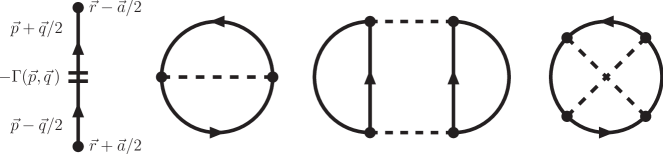
Figure 1: Left: The double-line symbolizes the medium insertion defined by eq.(4). Next are shown: The one-pion exchange Fock diagram and the iterated one-pion exchange Hartree and Fock diagrams.

3 Diagrammatic calculation

In this section we present analytical formulas for the three density-dependent strength functions $G_{d}(\rho)$, $G_{so}(\rho)$ and $G_{J}(\rho)$ as derived (via the improved density-matrix expansion [16]) from $1\pi$-exchange, iterated $1\pi$-exchange, and irreducible $2\pi$-exchange diagrams with intermediate $\Delta$-isobar excitations, including Pauli-blocking corrections up to three-loop order. We give for each diagram only the final result omitting all technical details related to extensive algebraic manipulations and solving elementary integrals. In essence the calculation of ref.[17] gets just modified by relative isospin factors $-1/3,\,\pm 2/3,\,-5/3$ occurring at various places.

3.1 One-pion exchange Fock diagram

The non-vanishing contribution from the $1\pi$-exchange Fock diagram shown in Fig. 1 reads:

$$G_{J}(\rho)={3g_{A}^{2}\over(32m_{\pi}f_{\pi})^{2}u^{6}}\Big{[}4u^{2}-8u^{4}-\ln(1+4u^{2})\Big{]}\,,$$ (5)

where we have introduced the convenient dimensionless variable $u=k_{f}/m_{\pi}$. This contribution to $G_{J}(\rho)$ is just $-1/3$ of the contribution to the isoscalar strength function $F_{J}(\rho)$ (see eq.(11) in ref.[17]) as a consequence of the isospin trace: tr$[\tau_{a}(J_{s}+\tau_{3}J_{v})\tau_{a}(J_{s}+\tau_{3}J_{v})]=6J_{s}^{2}-2J_{v}^{2}$.

3.2 Iterated $1\pi$-exchange Hartree diagram with two medium insertions

The two-body contributions from the iterated $1\pi$-exchange Hartree diagram in Fig. 1 read:

$$G_{d}(\rho)={g_{A}^{4}M\over 3\pi m_{\pi}(4f_{\pi})^{4}}\bigg{\{}{23\over 8u^{2}}\ln(1+4u^{2})-{8\over u}\arctan 2u+{3+20u^{2}\over 6(1+4u^{2})^{2}}\bigg{\}}\,,$$ (6)

$$G_{so}(\rho)={g_{A}^{4}M\over\pi m_{\pi}(4f_{\pi}u)^{4}}\bigg{\{}6u^{2}+{5\over 2}\ln(1+4u^{2})-8u\arctan 2u\bigg{\}}\,,$$ (7)

which are $-2/3$ of the respective isoscalar contributions [17, 20]. Let us briefly explain the mechanism which generates the strength function $G_{d}(\rho)$. The exchanged pion-pair transfers the momentum $\vec{q}$ between the left and the right nucleon ring. This momentum $\vec{q}$ enters both the pseudovector $\pi N$-interaction vertices and the pion propagators. After expanding the inner loop integral to order $\vec{q}\,^{2}$ the Fourier transformation in eq.(4) converts this factor $\vec{q}\,^{2}$ into a factor $(\vec{\nabla}k_{p}-\vec{\nabla}k_{n})^{2}\simeq\pi^{4}(\vec{\nabla}\rho_{p}-\vec{\nabla}\rho_{n})^{2}/k_{f}^{4}$. The rest is a solvable integral over the product of two Fermi spheres of radius $k_{f}$. The isovector spin-orbit strength function $G_{so}(\rho)$ arises from the spin-trace: tr$[\vec{\sigma}\cdot(\vec{l}+\vec{q}/2)\,\vec{\sigma}\cdot(\vec{l}-\vec{q}/2)\,\vec{\sigma}\cdot(\vec{p}_{1,2}\times\vec{J}_{v})]=2i\,(\vec{q}\times\vec{l}\,)\cdot(\vec{p}_{1,2}\times\vec{J}_{v})$, where $\vec{q}$ gets again converted to $\vec{\nabla}k_{p}-\vec{\nabla}k_{n}\simeq\pi^{2}(\vec{\nabla}\rho_{p}-\vec{\nabla}\rho_{n})/k_{f}^{2}$ by Fourier transformation.

3.3 Iterated $1\pi$-exchange Fock diagram with two medium insertions

We find the following contributions from the right Fock diagram in Fig. 1 with two medium insertions on non-neighboring nucleon propagators:

$$G_{d}(\rho) = {5g_{A}^{4}M\over 3\pi m_{\pi}(8f_{\pi})^{4}}\bigg{\{}{4\over u}(2\arctan 2u-\arctan u)+{1\over u^{2}}\ln{(1+u^{2})^{2}\over(1+2u^{2})(1+4u^{2})}$$ (8)

$$-{4\over 1+2u^{2}}+{2\over u^{2}}\int_{0}^{u}\!dx\,{3+18x^{2}+16x^{4}\over(1+2x^{2})^{3}}\Big{[}\arctan x-\arctan 2x\Big{]}\bigg{\}}\,,$$

$$G_{so}(\rho) = {5g_{A}^{4}M\over 2\pi m_{\pi}(4f_{\pi}u)^{4}}\bigg{\{}-u^{2}+\int_{0}^{u}\!\!dx\,{1\over 1+2x^{2}}$$ (9)

$$\times\Big{[}(1+4x^{2})\arctan 2x-4x^{2}(1+x^{2})\arctan x\Big{]}\bigg{\}}\,,$$

$$G_{J}(\rho) = {15g_{A}^{4}M\over\pi m_{\pi}(8f_{\pi}u)^{4}}\bigg{\{}u^{2}+{2\over u^{2}}\int_{0}^{u}\!\!dx\,{1\over 1+2x^{2}}\Big{[}(x^{2}-u^{2})(1+4x^{2})\arctan 2x$$ (10)

$$+2(6x^{6}-2u^{2}x^{4}+6x^{4}-2u^{2}x^{2}+2x^{2}-u^{2})\arctan x\Big{]}\bigg{\}}\,.$$

One notices a relative isospin factor of $-5/3$ in comparison to the respective isoscalar contributions [17, 20] which comes from the isospin trace tr$[\tau_{a}(J_{s}+\tau_{3}J_{v})\tau_{b}\tau_{a}(J_{s}+\tau_{3}J_{v})\tau_{b}]=10J_{v}^{2}-6J_{s}^{2}$ of this diagram.

3.4 Iterated $1\pi$-exchange Hartree diagram with three medium insertions

In our way of organizing the many-body calculation, the Pauli-blocking corrections are represented by diagrams with three medium insertions. The corresponding contributions from the iterated $1\pi$-exchange Hartree diagram shown in Fig. 1 read:

$$G_{d}(\rho) = {2g_{A}^{4}M\over 3\pi^{2}m_{\pi}(4f_{\pi})^{4}}\Bigg{\{}{1\over u}\int_{0}^{1}\!\!dy\,\ln{1+y\over 1-y}\bigg{[}{4u^{2}y^{2}(6+51u^{2}y^{2}+92u^{4}y^{4})\over 3(1+4u^{2}y^{2})^{3}}$$ (11)

$$-2\ln(1+4u^{2}y^{2})\bigg{]}+\int_{0}^{u}\!\!dx\,{x^{2}\over u^{4}}\int_{-1}^{1}\!\!dy\,{s^{3}s^{\prime}(3+9s^{2}+4s^{4})\over(1+s^{2})^{4}}\ln{u+xy\over u-xy}\Bigg{\}}\,,$$

$$G_{so}(\rho) = {2g_{A}^{4}M\over\pi^{2}m_{\pi}(4f_{\pi})^{4}}\int_{0}^{u}\!\!dx\,{x^{2}\over u^{6}}\int_{-1}^{1}\!\!dy\,\Bigg{\{}\bigg{[}4xy\ln{u+xy\over u-xy}+{u(5x^{2}y^{2}-3u^{2})\over u^{2}-x^{2}y^{2}}\bigg{]}$$ (12)

$$\times\bigg{[}5s+{s\over(1+s^{2})^{2}}-6\arctan s\bigg{]}-{us^{5}(u^{2}+x^{2}y^{2})\over(1+s^{2})^{2}(u^{2}-x^{2}y^{2})}$$

$$+{2s^{4}s^{\prime}\over(1+s^{2})^{2}}\bigg{[}4u-(s+2xy)\ln{u+xy\over u-xy}\bigg{]}\Bigg{\}}\,,$$

$$G_{J}(\rho)={3g_{A}^{4}Mu^{3}\over 16\pi^{2}m_{\pi}f_{\pi}^{4}}\int_{0}^{1}\!\!dy\,{y^{6}\over(1+4u^{2}y^{2})^{2}}\bigg{[}-2y+(y^{2}-1)\ln{1+y\over 1-y}\bigg{]}\,.$$ (13)

with the auxiliary function $s=xy+\sqrt{u^{2}-x^{2}+x^{2}y^{2}}$ and its partial derivative $s^{\prime}=u\,\partial s/\partial u$.

3.5 Iterated $1\pi$-exchange Fock diagram with three medium insertions

The evaluation of this diagram is most tedious. It is advisable to split the contributions to the strength functions $G_{d}(\rho)$, $G_{so}(\rho)$ and $G_{J}(\rho)$ into ”factorizable” and ”non-factorizable” parts. These two pieces are distinguished by the feature of whether the nucleon propagator in the denominator can be canceled or not by terms from the product of $\pi N$-interaction vertices in the numerator. We find the following ”factorizable” contributions:

$$G_{d}(\rho) = {g_{A}^{4}M\over 6\pi^{2}m_{\pi}(4f_{\pi})^{4}}\Bigg{\{}{95\arctan 2u\over 8(1+u^{2})}-{1+6u^{2}\over 32u^{5}}\ln^{2}(1+4u^{2})$$ (14)

$$+{9+100u^{2}+184u^{4}-192u^{6}\over 16u^{3}(1+u^{2})(1+4u^{2})}\ln(1+4u^{2})-{7u\over 1+4u^{2}}-{7\over 4u}$$

$$+{5\over u^{2}}\int_{0}^{u}\!dx\,\bigg{\{}-{L^{2}\over x^{2}}(1+u^{2})(3+3u^{2}+x^{2})-{3u^{2}\over x^{2}}+L\bigg{[}4u+{6u\over x^{2}}(1+u^{2})$$

$$+{x-4u\over 1+(u+x)^{2}}-{x+4u\over 1+(u-x)^{2}}+{2x\over[1+(u+x)^{2}]^{2}}-{2x\over[1+(u-x)^{2}]^{2}}\bigg{]}\bigg{\}}\Bigg{\}}\,,$$

$$G_{so}(\rho) = {g_{A}^{4}M\over\pi^{2}m_{\pi}(8f_{\pi}u)^{4}}\Bigg{\{}4\Big{[}19u^{2}-\ln(1+4u^{2})\Big{]}\arctan 2u-60u^{3}-8u-{3\over u}$$ (15)

$$+{3+14u^{2}+2u^{4}\over 2u^{3}}\ln(1+4u^{2})-{3+20u^{2}+16u^{4}\over 16u^{5}}\ln^{2}(1+4u^{2})$$

$$+20\int_{0}^{u}\!\!dx\,\bigg{\{}L^{2}\Big{[}u^{4}-2u^{2}-3-3x^{-2}(1+u^{2})^{3}+(3+7u^{2})x^{2}-5x^{4}\Big{]}$$

$$+6ux^{-2}(1+u^{2})^{2}L-3u^{2}x^{-2}(1+u^{2})\bigg{\}}\Bigg{\}}\,,$$

$$G_{J}(\rho) = {3g_{A}^{4}M\over\pi^{2}m_{\pi}(8f_{\pi}u)^{4}}\Bigg{\{}{185u\over 4}-4u^{3}-35\arctan 2u+{1+4u^{2}\over 16u^{5}}\ln^{2}(1+4u^{2})$$ (16)

$$+{1\over u}+{99u^{2}-8-68u^{4}\over 16u^{3}}\ln(1+4u^{2})+5\int_{0}^{u}\!\!dx\,\bigg{\{}{L^{2}\over u^{2}}\bigg{[}-{3\over 2x^{2}}(1+u^{2})^{4}$$

$$+2(u^{4}-1)(1+u^{2})-(5+2u^{2}+5u^{4})x^{2}+(6+10u^{2})x^{4}-{11x^{6}\over 2}\bigg{]}$$

$$+{L\over u}\bigg{[}{3\over x^{2}}(1+u^{2})^{3}-3u^{4}-2u^{2}+1\bigg{]}-{3\over 2x^{2}}(1+u^{2})^{2}\bigg{\}}\Bigg{\}}\,.$$

with the logarithmic function:

$$L(x,u)={1\over 4x}\ln{1+(u+x)^{2}\over 1+(u-x)^{2}}\,.$$ (17)

The ”non-factorizable” contributions (stemming from nine-dimensional principal value integrals over the product of three Fermi-spheres of radius $k_{f}$) read on the other hand:

$$G_{d}(\rho) = {g_{A}^{4}M\over 3\pi^{2}m_{\pi}(4f_{\pi})^{4}}\int_{-1}^{1}\!\!dy\int_{-1}^{1}\!\!dz\,{yz\,\theta(y^{2}+z^{2}-1)\over|yz|\sqrt{y^{2}+z^{2}-1}}\bigg{\{}{2uy^{2}\,\theta(y)\theta(z)\over 1+4u^{2}y^{2}}$$ (18)

$$\times\bigg{[}{2u^{2}z^{2}(3+4u^{2}z^{2})\over(1+4u^{2}z^{2})^{2}}-\ln(1+4u^{2}z^{2})\bigg{]}+\int_{0}^{u}\!\!dx\,{5x^{2}ss^{\prime}t^{3}t^{\prime}(1-5s^{2}-2s^{4})\over 4u^{6}(1+s^{2})^{3}(1+t^{2})}\bigg{\}}\,,$$

$$G_{so}(\rho) = {g_{A}^{4}M\over\pi^{2}m_{\pi}(4f_{\pi})^{4}}\int_{-1}^{1}\!\!dy\int_{-1}^{1}\!\!dz\,{yz\,\theta(y^{2}+z^{2}-1)\over|yz|\sqrt{y^{2}+z^{2}-1}}\bigg{\{}{8y^{2}z\,\theta(y)\theta(z)\over 1+4u^{2}y^{2}}$$ (19)

$$\times\Big{[}2uz-\arctan(2uz)\Big{]}+\int_{0}^{u}\!\!dx\,{5x^{2}s^{2}s^{\prime}t^{2}t^{\prime}\over 2u^{8}(1+s^{2})(1+t^{2})}(st+sxz-txy)\bigg{\}}\,,$$

$$G_{J}(\rho) = {3g_{A}^{4}M\over\pi^{2}m_{\pi}(4f_{\pi})^{4}}\int_{-1}^{1}\!\!dy\int_{-1}^{1}\!\!dz\,{yz\,\theta(y^{2}+z^{2}-1)\over|yz|\sqrt{y^{2}+z^{2}-1}}\bigg{\{}{2y^{4}\,\theta(y)\theta(z)\over u(1+4u^{2}y^{2})}$$ (20)

$$\times\Big{[}4u^{2}z^{2}-\ln(1+4u^{2}z^{2})\Big{]}+\int_{0}^{u}\!\!dx\,{5x^{4}s^{3}s^{\prime}t^{3}t^{\prime}(y^{2}+z^{2}-1)\over 4u^{10}(1+s^{2})(1+t^{2})}\bigg{\}}\,,$$

with the auxiliary function $t=xz+\sqrt{u^{2}-x^{2}+x^{2}z^{2}}$ and its partial derivative $t^{\prime}=u\,\partial t/\partial u$. For the numerical evaluation of the $dy\,dz$-double integrals in eqs.(18,19,20) it is advantageous to first antisymmetrize the integrands in $y$ and $z$ and then to substitute $z=\sqrt{y^{2}\zeta^{2}+1-y^{2}}$. This way the integration region becomes equal to the unit-square $0<y,\zeta<1$.

3.6 Irreducible two-pion exchange

At next order in the small momentum expansion comes the irreducible $2\pi$-exchange including (also) intermediate $\Delta$-isobar excitations. We employ a (subtracted) spectral-function representation of the $\pi N\Delta$-loops and find the following non-vanishing (two-body) contribution:

$$G_{J}(\rho) = {3\over 16\pi}\int_{2m_{\pi}}^{\infty}\!\!d\mu\,\Bigg{\{}{\rm Im}(V_{C}-W_{C})\bigg{[}{\mu\over 4k_{f}^{6}}(\mu^{2}+2k_{f}^{2})\ln\bigg{(}1+{4k_{f}^{2}\over\mu^{2}}\bigg{)}-{\mu\over k_{f}^{4}}-{4\over 3\mu^{3}}\bigg{]}$$ (21)

$$+{\rm Im}(V_{T}-W_{T})\bigg{[}{\mu\over k_{f}^{2}}-{4\over 3\mu}+{\mu^{3}\over 2k_{f}^{4}}-{\mu^{3}\over 8k_{f}^{6}}(\mu^{2}+4k_{f}^{2})\ln\bigg{(}1+{4k_{f}^{2}\over\mu^{2}}\bigg{)}\bigg{]}\Bigg{\}}\,.$$

The imaginary parts Im$V_{C}$, Im$W_{C}$, Im$V_{T}$ and Im$W_{T}$ of the isoscalar and isovector central and tensor NN-amplitudes due to $2\pi$-exchange with single and double $\Delta$-excitation can be found in section 3 of ref.[21]. The additional contributions from the irreducible $2\pi$-exchange with only nucleon intermediate states are accounted for by inserting into eq.(21) the imaginary parts:

$${\rm Im}W_{C}={\sqrt{\mu^{2}-4m_{\pi}^{2}}\over 3\pi\mu(4f_{\pi})^{4}}\bigg{[}4m_{\pi}^{2}(1+4g_{A}^{2}-5g_{A}^{4})+\mu^{2}(23g_{A}^{4}-10g_{A}^{2}-1)+{48g_{A}^{4}m_{\pi}^{4}\over\mu^{2}-4m_{\pi}^{2}}\bigg{]}\,,$$ (22)

$${\rm Im}V_{T}=-{6g_{A}^{4}\sqrt{\mu^{2}-4m_{\pi}^{2}}\over\pi\mu(4f_{\pi})^{4}}\,.$$ (23)

At leading order the irreducible $2\pi$-exchange generates no spin-orbit NN-interaction. It emerges first as a relativistic $1/M$-correction. In order to see the size of such relativistic effects we have evaluated the energy density functional with a two-body interaction composed of the (isoscalar and isovector) spin-orbit NN-amplitudes $V_{\rm SO}$ and $W_{\rm SO}$ written in eqs.(22,23) of ref.[22]. We find with it the following contribution to the isovector spin-orbit coupling strength:

$$G_{so}(\rho) = {g_{A}^{2}m_{\pi}\over\pi M(4f_{\pi})^{4}}\bigg{\{}{4-g_{A}^{2}\over 15u^{4}}\Big{[}\ln(1+u^{2})-u^{2}\Big{]}+{3\over 10}(11g_{A}^{2}-4)$$ (24)

$$+\bigg{[}{4-10g_{A}^{2}\over 3u}+{4u\over 5}(1-4g_{A}^{2})\bigg{]}\arctan u\bigg{\}}\,,$$

which has been subtracted at $\rho=0$ in order to eliminate (regularization dependent) short-distance components. As a consequence of that subtraction only the Fock terms are included in the expressions in eqs.(21,24).

3.7 Three-body diagrams with $\Delta$-excitation

Figure 2: Hartree and Fock three-body diagrams related to $2\pi$-exchange with virtual $\Delta$-isobar excitation (”Fujita-Miyazawa [23] mechanism”).

The Pauli-blocking correction to the $2\pi$-exchange with single $\Delta$-excitation is equivalent to the contribution of a (genuine) three-nucleon force. In fact, one is dealing here with the same three-nucleon interaction as originally introduced by Fujita and Miyazawa [23]. The pertinent Hartree and Fock three-body diagrams related to $2\pi$-exchange with virtual $\Delta$-excitation are shown in Fig. 2. Returning to the medium insertion written in eq.(4) we find from the left three-body Hartree diagram in Fig. 2 the following (non-vanishing) contribution:

$$G_{J}(\rho)={g_{A}^{4}m_{\pi}\over\pi^{2}\Delta(4f_{\pi})^{4}}\bigg{\{}{6\over u}-4u-{8u\over 1+4u^{2}}-{3\over 2u^{3}}\ln(1+4u^{2})\bigg{\}}\,,$$ (25)

with $\Delta=293\,$MeV the delta-nucleon mass splitting. We have used the value $3/\sqrt{2}$ for the ratio between the $\pi N\Delta$- and $\pi NN$-coupling constants. The vanishing of contributions to $G_{d}(\rho)$ and $G_{so}(\rho)$ has the following reason. The pertinent isospin trace generates an expression that is odd under exchange of the momenta $\vec{p}_{1}$ and $\vec{p}_{2}$ attached to the (upward and downward running) nucleon lines of the (left) closed nucleon ring. The remaining factor from the two-pion exchange interaction is however even (under $\vec{p}_{1}\leftrightarrow\vec{p}_{2}$) and so the whole expression integrates to zero.

The three-body effects on the energy density functional ${\cal E}_{\rm iv}[\rho_{p},\rho_{n},\vec{J}_{p},\vec{J}_{n}]$ are completed by the contributions from the central and right Fock diagrams in Fig. 2, which read:

$$G_{d}(\rho) = {g_{A}^{4}m_{\pi}\over 3\pi^{2}\Delta(8f_{\pi})^{4}}\Bigg{\{}{112u\over 1+4u^{2}}-16u-{20\over u}+{30\over u^{3}}$$ (26)

$$+\bigg{(}{64u\over 1+4u^{2}}-{14\over u}-{20\over u^{3}}-{15\over u^{5}}\bigg{)}\ln(1+4u^{2})$$

$$+{5\over 8u^{7}}(3+10u^{2}+8u^{4})\ln^{2}(1+4u^{2})\Bigg{\}}\,,$$

$$G_{so}(\rho) = {7g_{A}^{4}m_{\pi}\over\pi^{2}\Delta(8f_{\pi})^{4}}\Bigg{\{}{64u\over 9}-{4\over 3u}-{7\over 3u^{3}}-{4\over u^{5}}-{5\over 4u^{7}}$$ (27)

$$+\bigg{(}{5\over 8u^{9}}+{13\over 4u^{7}}+{13\over 3u^{5}}+{2\over u^{3}}-{8\over 3u}\bigg{)}\ln(1+4u^{2})$$

$$-{1\over 64u^{11}}(64u^{6}+80u^{4}+36u^{2}+5)\ln^{2}(1+4u^{2})\Bigg{\}}\,,$$

$$G_{J}(\rho) = {g_{A}^{4}m_{\pi}\over\pi^{2}\Delta(8f_{\pi}u)^{4}}\Bigg{\{}\bigg{[}{107u^{4}\over 2}+{217u^{2}\over 4}-{377\over 4}+{8\over u^{2}}\ln(1+4u^{2})\bigg{]}\arctan 2u$$ (28)

$$+\bigg{(}{3\over 8u^{5}}+{5\over 4u^{3}}+{737\over 64u}-{3547u\over 192}+{81u^{3}\over 16}\bigg{)}\ln(1+4u^{2})-{3\over 4u^{3}}-{1\over u}$$

$$+{787u\over 16}-{3935u^{3}\over 48}-{1696u^{5}\over 15}-{3+16u^{2}+144u^{4}\over 64u^{7}}\ln^{2}(1+4u^{2})$$

$$+\int_{0}^{u}\!\!dx\,\bigg{\{}{3L^{2}\over 8u^{2}}\bigg{[}{42\over x^{2}}(1+u^{2})^{4}(3u^{2}-1)-{35\over x^{4}}(1+u^{2})^{6}+(1+u^{2})^{2}$$

$$\times(94u^{2}-145-257u^{4})+4x^{2}(117u^{6}+35u^{4}-145u^{2}-63)-103x^{8}$$

$$+x^{4}(182u^{2}-165-597u^{4})+2x^{6}(199u^{2}-77)\bigg{]}+{L\over 4u}\bigg{[}{105\over x^{4}}(1+u^{2})^{5}$$

$$+{7\over x^{2}}(1+u^{2})^{3}(3-49u^{2})+18(1+u^{2})(37u^{4}-4u^{2}+23)\bigg{]}$$

$$-{105\over 8x^{4}}(1+u^{2})^{4}+{7\over 2x^{2}}(1+u^{2})^{2}(3+11u^{2})\bigg{\}}\Bigg{\}}\,,$$

with $L(x,u)$ defined in eq.(17). A good check of all formulas collected in this section is provided by their Taylor series expansion in $k_{f}$. Despite the superficial opposite appearance the leading term in the $k_{f}$-expansion is always a non-negative power of $k_{f}$ (which is higher for three-body contributions than for two-body contributions).

4 Results and discussion

In this section we present and discuss our numerical results obtained by summing the series of contributions given in section 3. The physical input parameters are: $g_{A}=1.3$ (nucleon axial vector coupling constant), $f_{\pi}=92.4\,$MeV (pion decay constant), $m_{\pi}=135\,$MeV (neutral pion mass) and $M=939\,$MeV (nucleon mass). We recall that with these physical parameters and a few adjustable short-distance couplings the nuclear matter equation of state $\bar{E}(\rho)$ and many other nuclear matter properties [24] can be well described by the chiral pion-nucleon dynamics treated up to three-loop order.

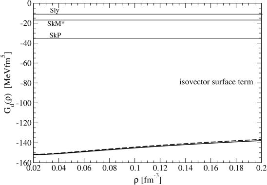
Figure 3: Strength function $G_{d}(\rho)$ of the isovector surface term $(\vec{\nabla}\rho_{p}-\vec{\nabla}\rho_{n})^{2}$ in the nuclear energy density functional versus the nucleon density $\rho=2k_{f}^{3}/3\pi^{2}$. Dashed line: Iterated $1\pi$-exchange only. Full line: $2\pi$-exchange and associated three-body contributions added.

Fig. 3 shows the strength function $G_{d}(\rho)$ belonging to the isovector surface term $(\vec{\nabla}\rho_{p}-\vec{\nabla}\rho_{n})^{2}$ plotted versus the nucleon density $\rho=2k_{f}^{3}/3\pi^{2}$. One observes that the leading result due to the iterated $1\pi$-exchange (eqs.(6,8,11,14,18) shown separately by the dashed line) is almost not changed by the inclusion of three-body contribution eq.(26) related to $2\pi$-exchange with virtual $\Delta$-excitation. Moreover, the density dependence of $G_{d}(\rho)$ is rather weak in the entire region $0<\rho<0.2\,{\rm fm}^{-3}$. The horizontal lines in Fig. 3 correspond to the (constant) values $G_{d}^{(\rm Sk)}=-[3t_{1}(2x_{1}+1)+t_{2}(2x_{2}+1)]/64$ of three phenomenological Skyrme forces SkM^∗ [3], SkP [4] and Sly [5]. These values are of the same negative sign, but considerably smaller in magnitude than our parameter-free prediction resulting from the long-range pion-exchange dynamics in the nuclear medium. It remains to be seen how well these (predicted) much larger negative values of $G_{d}(\rho)$, which energetically favor large differences in the density-gradients of protons and neutrons, perform in actual nuclear structure calculations at large neutron excess.

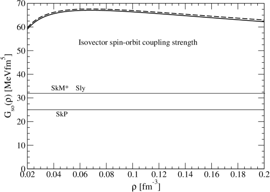
Figure 4: Strength function $G_{so}(\rho)$ of the isovector spin-orbit coupling term $(\vec{\nabla}\rho_{p}-\vec{\nabla}\rho_{n})\cdot(\vec{J}_{p}-\vec{J}_{n})$ in the nuclear energy density functional versus the nucleon density $\rho=2k_{f}^{3}/3\pi^{2}$. Dashed line: Iterated $1\pi$-exchange only. Full line: $2\pi$-exchange and three-body contributions added.

Of particular interest is the strength function $G_{so}(\rho)$ of the isovector spin-orbit coupling term $(\vec{\nabla}\rho_{p}-\vec{\nabla}\rho_{n})\cdot(\vec{J}_{p}-\vec{J}_{n})$ as provided by the explicit pion-exchange dynamics. As one can see from Fig. 4 the leading result due to the iterated $1\pi$-exchange (eqs.(7,9,12,15,19) shown separately by the dashed line) is again not changed by the inclusion of the $2\pi$-exchange and associated three-body contributions eqs.(24,27). This feature is markedly different from the isoscalar spin-orbit coupling strength $F_{so}(\rho)$ where an almost complete cancellation between these two components has occurred around $\rho_{0}/2=0.08\,{\rm fm}^{-3}$ (see Fig. 5 in ref.[17]). The basic reason for this totally different behavior is the absence of a strong isovector three-body spin-orbit coupling arising through the Fujita-Miyazawa mechanism (i.e. from the dominant three-body Hartree diagram in Fig. 2). There is of course in addition the short-range spin-orbit interaction which has to account practically for the full strength $F_{so}^{(\rm emp)}\simeq 90\,$MeVfm⁵ in the isoscalar channel and which contributes also in the isovector channel with a reduced weight $1/3$. Combined with our result for $G_{so}(\rho)$ from the long-range pion-exchange dynamics one would then have a situation where the isoscalar and isovector spin-orbit coupling strengths are about equally strong. As discussed in ref.[25] the isotope shifts of the charge radii in the Pb region (i.e. around the shell-closure $N=126$) can provide a sensitive test for strength of the isovector spin-orbit coupling. However, according to their limited analysis (in the vicinity of the stability line) no definite choice could be made between several density-dependences of the neutron spin-orbit potential: $\sim\rho_{p}+2\rho_{n}$ for the Skyrme force, $\sim\rho_{p}+\rho_{n}$ for the relativistic mean-field model, or $\sim\rho_{p}$ for the generalized functional SkI4 [25]. It remains to be seen whether the proportionality of the neutron spin-orbit potential to the gradient of the neutron density $\vec{\nabla}\rho_{n}$ as suggested by the present calculation leads to results which are in accordance with the existing precise experimental data.

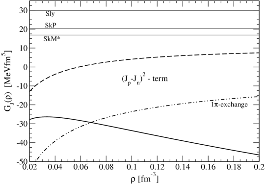
Figure 5: Strength function $G_{J}(\rho)$ belonging to the squared isovector spin-orbit density $(\vec{J}_{p}-\vec{J}_{n})^{2}$ in the nuclear energy density functional versus the nucleon density $\rho=2k_{f}^{3}/3\pi^{2}$. Dashed line: $1\pi$- and iterated $1\pi$-exchange only. Full line: $2\pi$-exchange and three-body contributions added.

Finally, we show in Fig. 5 the strength function $G_{J}(\rho)$ belonging the squared isovector spin-orbit density $(\vec{J}_{p}-\vec{J}_{n})^{2}$ in the nuclear energy density functional as a function of the nuclear density $\rho$. One observes that the inclusion of the subleading $2\pi$-exchange (two- and three-body) contributions eqs.(21,25,28) significantly affects the outcome for $G_{J}(\rho)$. For better orientation, we reproduce also by the dashed-dotted line in Fig. 5 the leading contribution from the $1\pi$-exchange Fock diagram alone (see eq.(5)). Interestingly, in the density region around $\rho_{0}/2=0.08\,{\rm fm}^{-3}$ the $1\pi$-exchange approximation and the complete result (full line) agree roughly with each other. The constant values $G_{J}^{(\rm Sk)}=(t_{1}-t_{2})/32$ from phenomenological Skyrme forces [3, 4, 5] are of similar magnitude but opposite in sign. Note that the strength function $G_{J}(\rho)$ comprises in particular the non-local Fock contributions from tensor forces, whose long-range isovector component is determined by the $1\pi$-exchange. This correspondence gives a rough understanding of the features visible in Fig. 5. Another interesting side effect of the $(\vec{J}_{p}-\vec{J}_{p})^{2}$ term in the nuclear energy density functional is that it gives rise to an extra spin-orbit mean-field $2G_{J}(\rho)\,(\vec{J}_{p}-\vec{J}_{n})$ in addition to the ”normal” one, $G_{so}(\rho)\,(\vec{\nabla}\rho_{p}-\vec{\nabla}\rho_{n})$. It would be interesting to investigate the role of this additional (nucleus-dependent) spin-orbit mean-field together with the density-dependence of $G_{J}(\rho)$ as predicted by in medium chiral perturbation theory.

In summary, we have used the improved density-matrix expansion of ref.[16] to calculate the strength functions of the isovector surface and spin-orbit terms in the nuclear energy density functional as provided by the long-range pion-exchange dynamics in the nuclear medium. These predictions together with the ones in ref.[17] for the isoscalar strength functions should be examined and explored in nuclear structure calculations at small and large neutron excess.

References

• [1] M. Bender, P.H. Heenen and P.G. Reinhard, Rev. Mod. Phys. 75 (2003) 121;
J.R. Stone and P.G. Reinhard, Prog. Part. Nucl. Phys. 58 (2007) 587.
• [2] M. Beiner, H. Flocard, N. Van Giai and P. Quentin, Nucl. Phys. A238 (1975) 29.
• [3] J. Bartel, P. Quentin, M. Brack, C. Guet and H.B. Hakansson, Nucl. Phys. A386 (1982) 79.
• [4] J. Dobaczewski, H. Flocard and J. Treiner, Nucl. Phys. A422 (1984) 103.
• [5] E. Chabanat, P. Bonche, P. Haensel, J. Meyer and R. Schaeffer, Nucl. Phys. A627 (1997) 710; A635 (1998) 231; and refs. therein.
• [6] S. Goriely, M. Samyn, M. Bender and J.M. Pearson, Phys. Rev. C68 (2003) 054325;
M. Samyn, S. Goriely, M. Bender and J.M. Pearson, Phys. Rev. C70 (2004) 044309;
N. Chamel, S. Goriely and J.M. Pearson, Nucl. Phys. A812 (2008) 72.
• [7] B.D. Serot and J.D. Walecka, Int. J. Mod. Phys. E6 (1997) 515; and refs. therein.
• [8] P. Ring, Lecture Notes in Physics, Vol.581, Springer-Verlag, Berlin, 2001, p. 195; and refs. therein.
• [9] P. Finelli, N. Kaiser, D. Vretenar and W. Weise, Nucl. Phys. A770 (2006) 1.
• [10] T. Lesinski, T. Duguet, K. Bennaceur and J. Meyer, Eur. Phys. J. A40 (2009) 121.
• [11] J.E. Drut, R.J. Furnstahl and L. Platter, Prog. Part. Nucl. Phys. 64 (2010) 120; nucl-th/0906.1463.
• [12] S.K. Bogner, R.J. Furnstahl and L. Platter, Eur. Phys. J. A39 (2009) 219.
• [13] S.K. Bogner, R.J. Furnstahl, A. Nogga and A. Schwenk, Nucl. Phys. A763 (2005) 59; nucl-th/0903.3366.
• [14] R. Roth, P. Papakonstantinou, N. Paar, H. Hergert, T. Neff and H. Feldmeier, Phys. Rev. C73 (2006) 044312.
• [15] J.W. Negele and D. Vautherin, Phys. Rev. C5 (1972) 1472.
• [16] B. Gebremariam, T. Duguet and S.K. Bogner, nucl-th/0910.4979.
• [17] N. Kaiser and W. Weise, Nucl. Phys. A (2010) in print; nucl-th/0912.3207.
• [18] N. Kaiser, Phys. Rev. C70 (2004) 034307.
• [19] O. Plohl and C. Fuchs, Phys. Rev. C74 (2006) 034325.
• [20] N. Kaiser, S. Fritsch and W. Weise, Nucl. Phys. A724 (2003) 47.
• [21] N. Kaiser, S. Gerstendörfer and W. Weise, Nucl. Phys. A637 (1998) 395.
• [22] N. Kaiser, R. Brockmann and W. Weise, Nucl. Phys. A625 (1997) 758.
• [23] J. Fujita and H. Miyawawa, Prog. Theor. Phys. 17 (1957) 360; 366.
• [24] S. Fritsch, N. Kaiser and W. Weise, Nucl. Phys. A750 (2005) 259.
• [25] P.G. Reinhart and H. Flocard, Nucl. Phys. A584 (1995) 467.