Global identifiability of linear structural equation models

Abstract

Structural equation models are multivariate statistical models that are defined by specifying noisy functional relationships among random variables. We consider the classical case of linear relationships and additive Gaussian noise terms. We give a necessary and sufficient condition for global identifiability of the model in terms of a mixed graph encoding the linear structural equations and the correlation structure of the error terms. Global identifiability is understood to mean injectivity of the parametrization of the model and is fundamental in particular for applicability of standard statistical methodology.

, and a1Supported by NSF Grant DMS-07-46265 and an Alfred P. Sloan Fellowship. a2Supported by NSF Grant DMS-08-40795 and the David and Lucille Packard Foundation.

1 Introduction

A mixed graph is a triple $G=(V,D,B)$ where $V$ is a finite set of nodes and $D,B\subseteq V\times V$ are two sets of edges. The edges in $D$ are directed, that is, $(i,j)\in D$ does not imply $(j,i)\in D$. We denote and draw such an edge as $i\to j$. The edges in $B$ have no orientation; they satisfy $(i,j)\in B$ if and only if $(j,i)\in B$. Following tradition in the field, we refer to these edges as bidirected and denote and draw them as $i\leftrightarrow j$. (In figures, we will draw bidirected edges also as dashed edges for better visual distinction.) We emphasize that in this setup the bidirected part $(V,B)$ is always a simple graph, that is, at most one bidirected edge may join a pair of nodes. Moreover, neither the bidirected part $(V,B)$ or the directed $(V,D)$ contain self-loops, that is, $(i,i)\notin D\cup B$ for all $i\in V$. In the main part of this work, the considered mixed graphs are acyclic, which means that the directed part $(V,D)$ is a directed graph without directed cycles.

Enumerate the vertex set as $V=[m]:=\{1,\ldots,m\}$. Let $\mathbb{R}^{D}$ be the set of matrices $\Lambda=(\lambda_{ij})\in\mathbb{R}^{m\times m}$ with $\lambda_{ij}=0$ if $i\to j$ is not in $D$. Write $\mathbb{R}^{D}_{\mathrm{reg}}$ for the subset of matrices $\Lambda\in\mathbb{R}^{D}$ for which $I-\Lambda$ is invertible, where $I$ denotes the identity matrix. Let $\mathit{PD}(m)$ be the cone of positive definite $m\times m$ matrices. Define $\mathit{PD}(B)$ to be the set of matrices $\Omega=(\omega_{ij})\in\mathit{PD}(m)$ with $\omega_{ij}=0$ if $i\not=j$ and $i\leftrightarrow j$ is not an edge in $B$. Write $\mathcal{N}_{m}(\mu,\Sigma)$ for the multivariate normal distribution with mean $\mu\in\mathbb{R}^{m}$ and covariance matrix $\Sigma$.

Definition 1.

The linear structural equation model $\mathcal{M}(G)$ associated with an acyclic mixed graph $G=(V,D,B)$ is the family of multivariate normal distributions $\mathcal{N}_{m}(0,\Sigma)$ with

$$\Sigma=(I-\Lambda)^{-T}\Omega(I-\Lambda)^{-1}$$

for $\Lambda\in\mathbb{R}^{D}_{\mathrm{reg}}$ and $\Omega\in\mathit{PD}(B)$.

The set of parents of a node $i$, denoted $\operatorname{pa}(i)$, comprises the nodes $j$ with $j\to i$ in $D$. The graphical model just defined is most naturally motivated in terms of a system of linear structural equations:

$$Y_{j}=\sum_{i\in\operatorname{pa}(j)}\lambda_{ij}Y_{i}+\varepsilon_{j},\qquad j=1,\ldots,m.$$ (1)

If $\varepsilon=(\varepsilon_{1},\ldots,\varepsilon_{m})$ is a random vector following the multivariate normal distribution $\mathcal{N}(0,\Omega)$ and $\Lambda\in\mathbb{R}^{D}_{\mathrm{reg}}$, then the random vector $Y=(Y_{1},\ldots,Y_{m})$ is well defined as a solution to the equation system in (1) and follows a centered multivariate normal distribution with covariance matrix $(I-\Lambda)^{-T}\Omega(I-\Lambda)^{-1}$.

Remark 1.

Assuming centered distributions presents no loss of generality. An arbitrary mean vector could be incorporated by adding an intercept constant $\lambda_{i0}$ to each equation in (1). The results discussed below would apply unchanged.

Linear structural equation models are ubiquitous in many applied fields, most notably in the social sciences where the models have a long tradition. Recent renewed interest in the models stems from their causal interpretability; compare spirtes2000 , pearl2009 . While current research is often concerned with non-Gaussian generalizations of the models, there remain important open problems about the linear Gaussian models from Definition 1. These include the following fundamental problem, which concerns the global identifiability of the model parameters.

Question 1.

For which mixed graphs $G=(V,D,B)$ is the rational parametrization

$$\phi_{G}\dvtx(\Lambda,\Omega)\mapsto(I-\Lambda)^{-T}\Omega(I-\Lambda)^{-1}$$

an injective map from $\mathbb{R}^{D}_{\mathrm{reg}}\times\mathit{PD}(B)$ to the positive definite cone $\mathit{PD}(m)$?

According to our first theorem, proven later on in Section 7, we can restrict attention to acyclic mixed graphs.

Theorem 1.

If $G$ is a mixed graph for which the parametrization $\phi_{G}$ is injective, then $G$ is acyclic.

The nodes of an acyclic mixed graph $G=(V,D,B)$ can be ordered topologically such that $i\to j\in D$ only if $i<j$. Under a topological ordering of the nodes, all matrices in $\mathbb{R}^{D}$ are strictly upper-triangular. Hence, $\mathbb{R}^{D}_{\mathrm{reg}}=\mathbb{R}^{D}$ because $\det(I-\Lambda)=1$ for all $\Lambda\in\mathbb{R}^{D}$. Moreover, the parametrization $\phi_{G}$ is a polynomial map in the entries of $\Lambda$ and $\Omega$ when $G$ is acyclic.

Characterizing the graphs with injective parametrization is important because failure of injectivity can lead to failure of standard statistical methods. We briefly exemplify this issue for the models considered here and point the reader to drtonlrt and references therein for a more detailed discussion. Briefly put, the problem is due to the fact that failure of injectivity can result in parameter spaces that are not smooth manifolds; compare in particular the examples in Section 1 of drtonlrt .

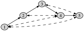
Figure 1: Acyclic mixed graph inducing a singular model.

(a)	(b)
(c)	(d)

Figure 2: Histograms of $p$-values for a likelihood ratio test.

Example 1.

Consider the graph $G=(V,D,B)$ from Figure 1. Let $\Lambda=(\lambda_{ij})$ be the matrix in $\mathbb{R}^{D}$ with

$$\lambda_{12}=3,\qquad\lambda_{23}=-\tfrac{1}{2},\qquad\lambda_{34}=\lambda_{45}=1.$$

Let $\Omega=(\omega_{ij})$ be the matrix in $\mathit{PD}(B)$ with all diagonal entries equal to 2 and

$$\omega_{14}=\omega_{15}=\omega_{24}=\omega_{35}=1.$$

It can be shown that at the specified point $(\Lambda,\Omega)$ the map $\phi_{G}$ is not injective and the image of $\phi_{G}$ has a singularity. Suppose we use the likelihood ratio test for testing the model $\mathcal{M}(G)$ against the saturated alternative given by all multivariate normal distributions on $\mathbb{R}^{m}$. The standard procedure would compare the resulting likelihood ratio statistic to a chi-square distribution with two degrees of freedom. Figure 2 illustrates the problems with this procedure. What is plotted are histograms of $p$-values obtained from the chi-square approximation. Each histogram is based on simulation of 20,000 samples of size $n=100$ or $n=1000$. The samples underlying the two histograms in Figure 2(a), (b) are drawn from the multivariate normal distribution with covariance matrix $\Sigma=\phi_{G}(\Lambda,\Omega)$ for the above parameter choices. Many $p$-values being large, it is evident that the test is too conservative. For comparison, we repeat the simulations with $\lambda_{23}=1/2$ and all other parameters unchanged. There is no identifiability failure in this second scenario, the image of $\phi_{G}$ is smooth in a neighborhood of the new covariance matrix and, as shown in Figure 2(c), (d), the expected uniform distribution for the $p$-values emerges in reasonable approximation.

Call a directed graph with at least two nodes an arborescence converging to node $i$ if its edges form a spanning tree with a directed path from any node $j\not=i$ to $i$. In other words, $i$ is the unique sink node. For a mixed graph $G=(V,D,B)$ and a subset of nodes $A\subset V$, let $D_{A}=D\cap(A\times A)$ be the set of directed edges with both endpoints in $A$. Similarly, let $B_{A}=B\cap(A\times A)$, and define the mixed subgraph induced by $A$ to be $G_{A}=(A,D_{A},B_{A})$. Our main result provides the following answer to Question 1.

Theorem 2.

The parametrization $\phi_{G}$ for an acyclic mixed graph $G=(V,D,B)$ fails to be injective if and only if there is an induced subgraph $G_{A}$, $A\subseteq V$, whose directed part $(A,D_{A})$ contains a converging arborescence and whose bidirected part $(A,B_{A})$ is connected. If $\phi_{G}$ is injective, then its inverse is a rational map.

An acyclic mixed graph $G=(V,D,B)$ is simple if there is at most one edge between any pair of nodes, that is, if $D\cap B=\varnothing$. Theorem 2 states in particular that only simple acyclic mixed graphs may have an injective parametrization. Indeed, two edges $i\leftrightarrow j$ and $i\to j$, respectively, connect and yield an arborescence in the subgraph $G_{\{i,j\}}$.

Corollary 1.

If the acyclic mixed graph $G$ has at most three nodes, then $\phi_{G}$ is injective if and only if $G$ is simple. There are exactly two unlabeled simple acyclic mixed graphs on four nodes with $\phi_{G}$ not injective.

An arborescence involving three nodes contains two edges. The bidirected part of a simple mixed graph can only be connected if there are two further edges. However, a simple graph with three nodes has at most three edges. The two examples on four nodes are shown in Figure 3.

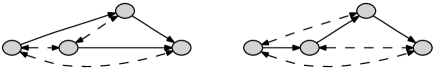
Figure 3: The two unlabeled graphs on four nodes with noninjective parametrization.

A possibly cyclic mixed graph $G=(V,D,B)$ is simple if there is at most one edge between any pair of nodes, that is, if $D\cap B=\varnothing$ and the presence of an edge $i\to j$ in $D$ implies the absence of $j\to i$. As shown in the next lemma, it is easy to give a direct proof of the fact that only simple graphs can have an injective parametrization. The lemma also clarifies that noninjectivity can be recognized in subgraphs, which is a fact that is important for later proofs.

Lemma 1.

Suppose the map $\phi_{G}$ given by a mixed graph $G$ is injective. Then $G$ is simple, and $\phi_{H}$ is injective for any (not necessarily induced ) subgraph $H$ of $G$.

If $H=(V^{\prime},D^{\prime},B^{\prime})$ is a subgraph of $G=(V,D,B)$, that is, $V^{\prime}\subseteq V$, $D^{\prime}\subseteq D$ and $B^{\prime}\subseteq B$, then $\phi_{H}$ is injective if and only if $\phi_{G}$ is injective at points that have all parameters $\lambda_{ij}$ and $\omega_{ij}$ zero for edges $(i,j)\in D\setminus D^{\prime}$ or $(i,j)\in B\setminus B^{\prime}$. If $G$ is not simple, then there exist two distinct indices $i,j$ for which the graph contains at least two of the three possible edges $i\to j$, $j\to i$ and $i\leftrightarrow j$. If $V=\{i,j\}$, then $\phi_{G}$ is not injective because it maps the at least 4-dimensional set $\mathbb{R}^{D}_{\mathrm{reg}}\times\mathit{PD}(B)$ to the 3-dimensional cone of positive definite $2\times 2$ matrices. If $|V|>2$, then the claim follows by passing to the subgraph induced by $\{i,j\}$.

The remainder of the paper is organized as follows. Section 2 reviews the connection of our work to the existing literature on identifiability of structural equation models. Section 3 lays out the natural stepwise approach to inversion of the parametrization $\phi_{G}$ in the case where the underlying graph is acyclic. Necessity and sufficiency of the graphical condition from our main Theorem 2 are proven in Sections 4 and 5, respectively. In Section 6, we collect three lemmas used in the proof of sufficiency. Theorem 1 about directed cycles is proven in Section 7. Concluding remarks are given in Section 8.

2 Prior work

Identifiability properties of structural equation models are a topic with a long history. A review of classical conditions, which do not take into account the finer graphical structure considered here, can be found, for instance, in the monograph bollen1989 . A more recent sufficient condition for global identifiability of the linear structural equation models from Definition 1 is due to mcdonald2002 , richardson2002 . It requires the presence of a bidirected edge $i\leftrightarrow j$ to imply the absence of directed paths from $j$ to $i$ (and from $i$ to $j$). Following richardson2002 , we call an acyclic mixed graph with this property ancestral. It is clear that an ancestral mixed graph is simple. We revisit the result about ancestral graphs in Corollary 2 below.

Other recent work, such as brito2002 , considers a weaker identifiability requirement for the model $\mathcal{M}(G)$ associated with a mixed graph $G=(V,D,B)$. For a pair of matrices $\Lambda_{0}\in\mathbb{R}^{D}_{\mathrm{reg}}$ and $\Omega_{0}\in\mathit{PD}(B)$, define the fiber

$$\qquad\mathcal{F}(\Lambda_{0},\Omega_{0})=\{(\Lambda,\Omega)\dvtx\phi_{G}(\Lambda,\Omega)=\phi_{G}(\Lambda_{0},\Omega_{0}),\Lambda\in\mathbb{R}^{D}_{\mathrm{reg}},\Omega\in\mathit{PD}(B)\}.$$ (2)

The map $\phi_{G}$ is injective if and only if all its fibers contain only a single point. If it holds instead that for generic choices of $\Lambda\in\mathbb{R}^{D}_{\mathrm{reg}}$ and $\Omega\in\mathit{PD}(B)$, the fiber $\mathcal{F}(\Lambda,\Omega)$ contains only the single point $(\Lambda,\Omega)$, then we say that the map $\phi_{G}$ is generically injective and the model $\mathcal{M}(G)$ is generically identifiable. Requiring a condition to hold for generic points means that the points at which the condition fails form a lower-dimensional algebraic subset. In particular, the condition holds for almost every point (in Lebesgue measure), and some authors thus also speak of an almost everywhere identifiable model; compare the lemma in okamoto1973 . When the substantive interest is in all parameters of a model, generic identifiability constitutes a minimal requirement. However, generically but not globally identifiable models can have nonsmooth parameter spaces and thus present difficulties for statistical inference; recall Example 1 that treats a generically identifiable model.

The main theorem of brito2002 , which we reprove in Corollary 3, states that $\phi_{G}$ is generically injective for every simple acyclic mixed graph $G$. The graph being simple and acyclic, however, is far from necessary for generic injectivity of $\phi_{G}$. A classical counterexample is the instrumental variable model based on the graph with edges $1\to 2\to 3$ and $2\leftrightarrow 3$. Cyclic models may also be generically identifiable; for instance, see Example 3.6 in drtonlrt . For recent work on the topic, see tian2009 and references therein. To our knowledge, characterizing the mixed graphs $G$ with generically injective parametrization $\phi_{G}$ remains an open problem.

The linear structural equation models $\mathcal{M}(G)$ considered in this paper are closely related to latent variable models known as semi-Markovian causal models. These nonparametric models are obtained by subdividing the bidirected edges, that is, each edge $i\leftrightarrow j$ is replaced by two directed edges $i\leftarrow u_{ij}\to j$, where $u_{ij}$ is a new node. Each node $u_{ij}$ added to the vertex set corresponds to a latent variable; compare also richardson2002 , pearl2009 , wermuth2010 . Using results from tian2002 , the work of shpitser2006 gives graphical conditions for when (univariate or multivariate) intervention distributions in acyclic semi-Markovian causal models are identified. This work is based on manipulating recursive density factorizations involving latent variables. If $G$ is an acyclic mixed graph and the structural equation model $\mathcal{M}(G)$ is contained in the semi-Markovian model for $G$, then $\mathcal{M}(G)$ is globally identified provided that in the semi-Markovian model we can identify, for every node $i$, the univariate intervention distribution for $i$ and intervention set $\operatorname{pa}(i)$; see also Chapter 6 in tian2002 .

For an acyclic mixed graph $G=(V,D,B)$, we may define a Gaussian model $\mathcal{M}^{\prime}(G)$ by assuming that both the observed and the latent variables in the semi-Markovian model for $G$ have a joint multivariate normal distribution. This creates an explicit connection to linear structural equation models, and it is indeed possible that $\mathcal{M}^{\prime}(G)=\mathcal{M}(G)$. For instance, if there are no directed edges $(D=\varnothing)$, then $\mathcal{M}^{\prime}(G)=\mathcal{M}(G)$ if and only if the bidirected part $(V,B)$ is a forest of trees; see Corollary 3.4 in drtonyu2010 . If $D=\varnothing$ and $(V,B)$ is not a forest of trees, then $\mathcal{M}(G)$ is strictly larger than $\mathcal{M}^{\prime}(G)$. Therefore, other nonnormal constructions would be required in order for the theorems in shpitser2006 to furnish sufficient conditions for global identifiability of linear structural equation models. We are unaware, however, of literature providing a connection between semi-Markovian causal models and the linear structural equation models from Definition 1 when non-Gaussian distributions are assumed for the latent variables.

Finally, the existing counterexamples to identifiability of semi-Markovian models involve binary variables and thus cannot be used to prove necessity of an identifiability condition for the Gaussian models $\mathcal{M}(G)$. However, despite this fact and the difficulties in relating the models $\mathcal{M}(G)$ to semi-Markovian models, our graphical condition from Theorem 2, which we first found by experimentation with computer algebra software, coincides with that of shpitser2006 ; the term “$y$-rooted C-tree” is used there to refer to a mixed graph whose directed part is an arborescence converging to node $y$ and whose bidirected part is a tree. A reader familiar with the work in tian2002 will also recognize similarities between the higher-level structure of the proofs given there and those in Section 5 of this paper.

3 Stepwise inversion

Throughout this section, suppose that $G\!=\!(\!V,D,B\!)$ is an acyclic mixed graph with vertex set $V=[m]$. The map $\phi_{G}$ is injective if all its fibers contain only a single point; recall the definition of a fiber in (2). Let $\Sigma=\phi_{G}(\Lambda_{0},\Omega_{0})$ for two matrices $\Lambda_{0}\in\mathbb{R}^{D}$ and $\Omega_{0}\in\mathit{PD}(B)$. This section describes how to find points $(\Lambda,\Omega)$ in the fiber $\mathcal{F}(\Lambda_{0},\Omega_{0})$. In particular, we show in Lemma 2 that an algebraic criterion can be used to decide whether the map $\phi_{G}$ is injective. The lemma is proven after we describe a natural inversion approach that uses the acyclic structure of the graph $G$ in a stepwise manner. We remark that this stepwise inversion is closely related to the idea of pseudo-variable regression used in the iterative conditional fitting algorithm of drtoneichler2009 .

For each $i\leq m-1$, let $P(i)=\operatorname{pa}(i+1)$ be the parents of node $i+1$, and $S(i)=\{j\leq i\dvtx j\leftrightarrow i+1\in B\}$ the siblings of $i+1$. (In other related work, the nodes incident to a bidirected edge $i\leftrightarrow j$ have also been called “spouses” of each other but we find “siblings” to be natural terminology given that a common parent to the two nodes is introduced when subdividing the edge as discussed in Section 2.)

Lemma 2.

Suppose $G=(V,D,B)$ is an acyclic mixed graph with its nodes labeled in a topological order. Then the parametrization $\phi_{G}$ is injective if and only if the rank condition

$$\operatorname{rank}\bigl{(}\Omega_{[i]\setminus S(i),[i]}(I-\Lambda)^{-1}_{[i],P(i)}\bigr{)}=|P(i)|$$

holds for all nodes $i=1,\ldots,m-1$ and all pairs $\Lambda\in\mathbb{R}^{D}$ and $\Omega\in\mathit{PD}(B)$.

Remark 2.

In this paper, matrix inversion is always given higher priority than an operation of forming a submatrix. For any invertible matrix $M$ and index sets $A,B$, the matrix $M^{-1}_{A,B}=(M^{-1})_{A,B}$ is thus the $A\times B$ submatrix of the inverse of $M$.

Computing points $(\Lambda,\Omega)$ in the fiber $\mathcal{F}(\Lambda_{0},\Omega_{0})$ means solving the polynomial equation system given by the matrix equation

$$\Sigma=(I-\Lambda)^{-T}\Omega(I-\Lambda)^{-1}.$$ (3)

For topologically ordered nodes, (3) implies that $\sigma_{11}=\omega_{11}$ and that the first column in the strictly upper-triangular matrix $\Lambda$ contains only zeros. Hence, these are uniquely determined for all matrices in the fiber.

Let $i\geq 1$, and assume that we know the $[i]\times[i]$ submatrices of $\Lambda$ and $\Omega$ of a solution to equation (3). Partition off the $(i+1)$st row and column of the submatrices

$$(I-\Lambda)_{[i+1],[i+1]}=\pmatrix{\Gamma&-\lambda\cr 0&1},\qquad\Omega_{[i+1],[i+1]}=\pmatrix{\Psi&\omega\cr\omega^{T}&\omega_{i+1,i+1}}.$$

The matrices $\Gamma$ and $\Psi$ are known, $\lambda_{[i]\setminus P(i)}=0$ and $\omega_{[i]\setminus S(i)}=0$. The inverse of $I-\Lambda$ can be written as a block matrix as

$$(I-\Lambda)^{-1}_{[i+1],[i+1]}=\pmatrix{\Gamma^{-1}&\Gamma^{-1}\lambda\cr 0&1}.$$ (4)

In this notation, the part of equation (3) that pertains to the $[i+1]\times[i+1]$ submatrix of $\Sigma$ is

$$\pmatrix{\Sigma_{[i],[i]}&\Sigma_{[i],\{i+1\}}\cr&\sigma_{i+1,i+1}}$$

$$\qquad=\pmatrix{\Gamma^{-T}\Psi\Gamma^{-1}&\Gamma^{-T}\Psi\Gamma^{-1}\lambda+\Gamma^{-T}\omega\cr&\omega_{i+1,i+1}+\lambda^{T}\Gamma^{-T}\Psi\Gamma^{-1}\lambda+2\omega^{T}\Gamma^{-1}\lambda},$$

where only the upper-triangular parts of the symmetric matrices are shown. Hence, given the values of $\Gamma$ and $\Psi$, the choice of $\lambda$ and $\omega$ is unique if and only if the equation

$$\Sigma_{[i],\{i+1\}}=\Gamma^{-T}\Psi\Gamma^{-1}\cdot\lambda+\Gamma^{-T}\cdot\omega$$ (5)

has a unique solution. Clearly, any feasible choice of a solution $(\lambda,\omega)$ to the equation in (5) leads to a unique solution $\omega_{i+1,i+1}$ via the equation

$$\sigma_{i+1,i+1}=\omega_{i+1,i+1}+\lambda^{T}\Gamma^{-T}\Psi\Gamma^{-1}\lambda+2\omega^{T}\Gamma^{-1}\lambda.$$ (6)

Since $\lambda_{[i]\setminus P(i)}=0$ and $\omega_{[i]\setminus S(i)}=0$, equation (5) can be rewritten as

$$\Sigma_{[i],\{i+1\}}=\bigl{(}\Gamma^{-T}\Psi\Gamma^{-1}_{[i],P(i)}\bigr{)}\cdot\lambda_{P(i)}+\bigl{(}\Gamma^{-1}_{S(i),[i]}\bigr{)}^{T}\cdot\omega_{S(i)}.$$

It has a unique solution if and only if the matrix

$$\left[\vphantom{\bigl{(}\Gamma^{-1}_{S(i),[i]}\bigr{)}^{T}}\matrix{\Gamma^{-T}\Psi\Gamma^{-1}_{[i],P(i)}&\bigl{(}\Gamma^{-1}_{S(i),[i]}\bigr{)}^{T}}\right]$$

has full column rank $|P(i)|+|S(i)|$. The matrix $\Gamma$ is invertible because it is upper-triangular with ones along the diagonal. Thus, the condition is equivalent to

$$\Gamma^{T}\left[\vphantom{\bigl{(}\Gamma^{-1}_{S(i),[i]}\bigr{)}^{T}}\matrix{\Gamma^{-T}\Psi\Gamma^{-1}_{[i],P(i)}&\bigl{(}\Gamma^{-1}_{S(i),[i]}\bigr{)}^{T}}\right]=\left[\vphantom{\Psi\Gamma^{-1}_{[i],P(i)}}\matrix{\Psi\Gamma^{-1}_{[i],P(i)}&I_{[i],S(i)}}\right]$$

having full column rank. The second block is part of an identity matrix. We deduce that the condition is equivalent to requiring that $\Psi_{[i]\setminus S(i),[i]}\Gamma^{-1}_{[i],P(i)}$, the submatrix obtained by removing the rows and columns with index in $S(i)$, has rank $|P(i)|$. Note that

$$\Psi_{[i]\setminus S(i),[i]}\Gamma^{-1}_{[i],P(i)}=\Omega_{[i]\setminus S(i),[i]}(I-\Lambda)^{-1}_{[i],P(i)}$$

is the matrix appearing in Lemma 2.

Proof of Lemma 2 Consider a feasible pair $(\Lambda,\Omega)$. If the rank condition for this pair holds for all nodes $i=1,\ldots,m-1$, then it follows from the stepwise inversion procedure described above that the fiber $\mathcal{F}(\Lambda,\Omega)$ contains only the single point $(\Lambda,\Omega)$. Therefore, the rank condition holding for all nodes and all matrix pairs implies that all fibers are singletons, or in other words, that the map $\phi_{G}$ is injective.

Conversely, assume that the rank condition fails for some node $i\leq m-1$ and matrix pair $(\Lambda,\Omega)$. If $i=m-1$, then the considered fiber $\mathcal{F}(\Lambda,\Omega)$ is positive-dimensional, and $\phi_{G}$ not injective. If $i<m-1$, then it follows analogously that the parametrization $\phi_{H}$ for the induced subgraph $H=G_{[i+1]}$ is not injective. By Lemma 1, $\phi_{G}$ cannot be injective either.

If the rank condition in Lemma 2 holds at a particular pair $(\Lambda,\Omega)$, then the fiber $\mathcal{F}(\Lambda,\Omega)$ contains only the pair $(\Lambda,\Omega)$. However, the converse is false in general, that is, failure of the rank condition at a particular pair $(\Lambda,\Omega)$ and vertex $i<m$ need not imply that the fiber $\mathcal{F}(\Lambda,\Omega)$ contains more than one point. This may occur even for a simple acyclic mixed graph.

Example 2.

Consider the graph in Figure 4, set $\lambda_{12}=\lambda_{23}=\lambda_{34}=1$, and choose the positive definite matrix

$$\Omega=\pmatrix{2&0&-1&-1&-1\cr 0&1&0&-1&0\cr-1&0&1&0&0\cr-1&-1&0&3&0\cr-1&0&0&0&3}.$$

The rank condition for this pair $(\Lambda,\Omega)$ fails at node $i=3$. Nevertheless, the fiber $\mathcal{F}(\Lambda,\Omega)$ is equal to $\{(\Lambda,\Omega)\}$. If we set $\omega_{15}=0$, however, then $\mathcal{F}(\Lambda,\Omega)$ becomes one-dimensional. Using terminology from econometrics/causality, the variable corresponding to node 5 behaves like an “instrument;” compare, for instance, pearl2009 .

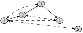
Figure 4: Graph with noninjective parametrization (see Example 2).

Lemma 2 allows us to give simple proofs of two established results in the graphical models literature. The proof of Corollary 2 emphasizes the special structure exhibited by ancestral graphs. The proof of Corollary 3 demonstrates that the identity matrix always has a singleton as a fiber under the parametrization associated with a simple acyclic mixed graph.

Corollary 2.

If the acyclic mixed graph $G$ is ancestral then the parametrization $\phi_{G}$ is injective.

Recall that if $G=(V,D,B)$ is ancestral and $i\leftrightarrow j$ is a bidirected edge in $G$, then there is no directed path from $i$ to $j$ or $j$ to $i$. Suppose $V=[m]$ is topologically ordered, and let $i$ be some node smaller than $m$. Pick a node $j\in S(i)$. Then there may not exist a directed path from $j$ to a node in $P(i)$. It follows that

$$\Omega_{[i]\setminus S(i),[i]}(I-\Lambda)^{-1}_{[i],P(i)}=\Omega_{[i]\setminus S(i),[i]\setminus S(i)}(I-\Lambda)^{-1}_{[i]\setminus S(i),P(i)}.$$

The latter matrix is the product of a principal and thus positive definite submatrix of $\Omega$ and a matrix that contains the $P(i)\times P(i)$ identity matrix. It follows that this product has full column rank $|P(i)|$ for all feasible pairs $(\Lambda,\Omega)$ and all nodes $i\leq m-1$. By Lemma 2, $\phi_{G}$ is injective.

If the acyclic mixed graph $G$ is simple, then $P(i)\subseteq[i]\setminus S(i)$ for all nodes $i\leq m-1$. Hence, the matrix product appearing in the rank condition always has at least as many rows as columns. The next generic identifiability result follows immediately; recall the definitions in Section 2.

Corollary 3.

If $G=(V,D,B)$ is a simple acyclic mixed graph, then the map $\phi_{G}$ is generically injective.

We need to show that for generic choices of $\Lambda\in\mathbb{R}^{D}$ and $\Omega\in\mathit{PD}(B)$, the fiber $\mathcal{F}(\Lambda,\Omega)$ is equal to the singleton $\{(\Lambda,\Omega)\}$. Set $\Lambda=0$ and choose $\Omega$ to be the identity matrix. Then each of the matrix products

$$\Omega_{[i]\setminus S(i),[i]}(I-\Lambda)^{-1}_{[i],P(i)},\qquad i=1,\ldots,m-1,$$ (7)

has the identity matrix as $P(i)\times P(i)$ submatrix. The rank condition from Lemma 2 thus holds for all $i\leq m-1$. Since the matrices in (7) have polynomial entries, existence of a single pair $(\Lambda,\Omega)$ at which the $m-1$ matrices in (7) have full column rank implies that the set of pairs $(\Lambda,\Omega)$ for which at least one of the matrices fails to have full column rank is a lower-dimensional algebraic set; compare cox2007 , Chapter 9, for background on such algebraic arguments.

In order to prepare for arguments turning the algebraic condition from Lemma 2 into a graphical one, we detail the structure of the inverse $(I-\Lambda)^{-1}$ for a matrix $\Lambda=(\lambda_{ij})\in\mathbb{R}^{D}$. Let $\mathcal{P}(i,j)$ denote the set of directed paths from $i$ to $j$ in the considered acyclic graph.

Lemma 3.

The entries of the inverse $(I-\Lambda)^{-1}$ are

$$(I-\Lambda)^{-1}_{ij}=\sum_{\pi\in\mathcal{P}(i,j)}\prod_{k\to l\in\pi}\lambda_{kl},\qquad i,j\in[m].$$

This well-known fact can be shown by induction on the matrix size $m$ and using the partitioning in (4) under a topological ordering of the nodes.

Note that adopting the usual definition that takes an empty sum to be zero and an empty product to be one, the formula in Lemma 3 states that $(I-\Lambda)^{-1}_{ij}=0$ if $i\not=j$ and $\mathcal{P}(i,j)=\varnothing$, and it states that $(I-\Lambda)^{-1}_{ii}=1$ because $\mathcal{P}(i,i)$ contains only a trivial path without edges.

4 Necessity of the graphical condition for identifiability

We now prove that the graphical condition in Theorem 2, which states that there be no induced subgraph whose directed part contains a converging arborescence and whose bidirected part is connected, is necessary for the parametrization $\phi_{G}$ to be injective. By Lemma 1, it suffices to consider an acyclic mixed graph whose directed part is a converging arborescence and whose bidirected part is a spanning tree. In light of Lemma 2, the necessity of the graphical condition in Theorem 2 then follows from the following result.

Proposition 1.

Let $G=(V,D,B)$ be an acyclic mixed graph with topologically ordered vertex set $V=[m+1]$. If $(V,D)$ is an arborescence converging to $m+1$ and $(V,B)$ is a spanning tree, then there exists a pair of matrices $\Lambda\in\mathbb{R}^{D}$ and $\Omega\in\mathit{PD}(B)$ with

$$\operatorname{kernel}\bigl{(}\Omega_{[m]\setminus S(m),[m]}(I-\Lambda)^{-1}_{[m],P(m)}\bigr{)}\not=\{0\}.$$

Let $\mathcal{L}(\Lambda)\subseteq\mathbb{R}^{m}$ be the column span of $(I-\Lambda)^{-1}_{[m],P(m)}$. We formulate a first lemma that we will use to prove Proposition 1.

Lemma 4.

If $V=[m+1]$ and $(V,D)$ is an arborescence converging to node $m+1$, then the union of the linear spaces $\mathcal{L}(\Lambda)$ for all $\Lambda\in\mathbb{R}^{D}$ contains the set $(\mathbb{R}^{*})^{m}=(\mathbb{R}\setminus\{0\})^{m}$ of vectors with all coordinates nonzero.

In the arborescence, there is a unique path $\pi(i)$ from any vertex $i\in[m]\setminus P(m)$ to the sink node $m+1$. Let $k(i)$ be the unique node in $P(m)$ that lies on this path. Let $\Lambda\in\mathbb{R}^{D}$ and $\alpha\in\mathbb{R}^{|P(m)|}$, and define the vector

$$\beta(\Lambda,\alpha)=(I-\Lambda)^{-1}_{[m],P(m)}\alpha\in\mathbb{R}^{m}.$$

Since the principal submatrix $(I-\Lambda)^{-1}_{P(m),P(m)}$ is an identity matrix (because the directed graph is a converging arborescence), $\beta(\Lambda,\alpha)_{i}=\alpha_{i}$ for all $i\in P(m)$. For $i\in[m]\setminus P(m)$, we use Lemma 3 to obtain

$$\beta(\Lambda,\alpha)_{i}=\alpha_{k(i)}\prod_{j\to l\in\pi(i)}\lambda_{jl}=\lambda_{ij}\beta(\Lambda,\alpha)_{j},$$ (8)

where $i\to j\in G$ is the unique edge originating from $i$.

Let $x$ be any vector in $(\mathbb{R}^{*})^{m}$. Our claim states that there exist a matrix $\Lambda\in\mathbb{R}^{D}$ and vector $\alpha$ such that $x=\beta(\Lambda,\alpha)$. Clearly, $\alpha$ has to be equal to the subvector $x_{P(m)}$. The associated unique choice of $\Lambda$ is obtained by recursively solving for the entries $\lambda_{ij}$ using the relationship in (8).

Let $R(m)=[m]\setminus S(m)$ be the “rest” of the nodes. We are left with the problem of finding a matrix $\Omega\in\mathit{PD}(B)$ for which some vector in $(\mathbb{R}^{*})^{m}$ lies in the kernel of the submatrix

$$\Omega_{R(m),[m]}=\left[\vphantom{\Omega_{R(m),R(m)}}\matrix{\Omega_{R(m),R(m)}&\Omega_{R(m),S(m)}}\right].$$

Proposition 1 now follows by combining Lemma 4 with the next result.

Lemma 5.

If $(V,B)$ is a tree on $V=[m+1]$, then there exists a matrix $\Omega\in\mathit{PD}(B)$ such that the vector $\mathbf{1}=(1,\ldots,1)^{T}$ is in the kernel of the submatrix $\Omega_{R(m),[m]}$.

Let $T$ be the set of all nodes in $R(m)$ that are connected to some node in $S(m)$ by an edge in $B$. If $\Omega\in\mathit{PD}(B)$, then the submatrix $\Omega_{R(m),S(m)}$ has only zero entries in rows indexed by nodes $i\in R(m)\setminus T$. If $i\in T$, then the $i$th row of $\Omega_{R(m),S(m)}$ has at least one entry that is not constrained to zero and may take any real value. Hence, we can choose a matrix $\Omega_{R(m),S(m)}$ that has row sum

$$\sum_{j\in S(m)}\omega_{ij}=\cases{\displaystyle-1,&\quad if $i\in T$,\cr\displaystyle 0,&\quad if $i\in R(m)\setminus T$.}$$ (9)

Let $H=(R(m),B_{R(m)})$ be the induced subgraph of $G$ on vertex set $R(m)$. The Laplacian of $H$, $L(H)=(l_{ij})$, is the symmetric $R(m)\times R(m)$ matrix whose diagonal entries are the degrees of the nodes in $H$ and whose off-diagonal entries $l_{ij}$ are equal to $-$1 if $i\leftrightarrow j$ is an edge in $H$ and 0 otherwise. The Laplacian is well known to be positive semidefinite with all row sums zero. For a subset $C\subset[m]$, let $\mathbf{1}_{C}\in\mathbb{R}^{m}$ be the vector with entries equal to one at indices in $C$ and zero elsewhere. The kernel of $L(H)$ is the direct sum of the linear spaces spanned by the vectors $\mathbf{1}_{C}$ for the connected components $C$ of the graph $H$; compare chung1997 , Chapter 1.

Let $D_{T}=(d_{ij})$ be the diagonal matrix that has diagonal entry $d_{ii}=1$ if $i\in T$ and $d_{ii}=0$ otherwise. Both $L(H)$ and $D_{T}$ are positive semidefinite matrices and thus the kernel of $L(H)+D_{T}$ is equal to $\ker L(H)\cap\ker D_{T}$. Since $(V,B)$ is a connected graph, each connected component of $H$ contains a node in $T$. Therefore, none of the vectors $\mathbf{1}_{C}$ are in the kernel of $D_{T}$, where $C$ ranges over all connected components of $H$. This implies that the $\ker(L(H)+D_{T})=\{0\}$, and hence this matrix is positive definite.

Let $\Omega$ be any matrix in $\mathit{PD}(B)$ whose submatrix $\Omega_{R(m),S(m)}$ satisfies (9) and whose principal submatrix $\Omega_{R(m),R(m)}$ is the positive definite matrix $L(H)+D_{T}$. The matrix $\Omega\in\mathit{PD}(B)$ has the desired property because

$$\Omega_{R(m),[m]}\mathbf{1}=\bigl{(}L(H)+D_{T}\bigr{)}\mathbf{1}+\Omega_{R(m),S(m)}\mathbf{1}=\mathbf{1}_{T}-\mathbf{1}_{T}=0.$$

Such matrices exist because we can choose $\Omega_{S(m),S(m)}$ to be, for instance, a diagonal matrix with very large diagonal entries. Principal minors of $\Omega$ that are not submatrices of $\Omega_{R(m),R(m)}$ will be dominated by these diagonal entries and hence be positive. All other principal minors are positive since $\Omega_{R(m),R(m)}=L(H)+D_{T}$ was shown to be positive definite.

5 Sufficiency of the graphical condition for identifiability

In this section, we prove that the graphical condition in Theorem 2, which requires an acyclic mixed graph $G$ to have no induced subgraph whose directed part contains a converging arborescence and whose bidirected part is connected, is sufficient for the parametrization $\phi_{G}$ to be injective. Proposition 4 below shows that if $\phi_{G}$ is not injective and $G$ does not contain an induced subgraph with both a converging arborescence and a bidirected spanning tree, then there is a subgraph $G^{\prime}$ with fewer nodes such that $\phi_{G^{\prime}}$ still fails to be injective. The sufficiency of the graphical condition then follows immediately. To see this, note that a graph $G$ with noninjective parametrization $\phi_{G}$ must contain some minimal induced subgraph $G^{\prime}$ with noninjective $\phi_{G^{\prime}}$. Applying the contrapositive of Proposition 4 to $G^{\prime}$, we conclude that the directed part of $G^{\prime}$ contains a converging arborescence and the bidirected part of $G^{\prime}$ is connected.

In preparing for the proof of Proposition 4, we first treat the case when there is no arborescence; this gives Proposition 2. The case when there is no bidirected spanning tree is treated in Proposition 3. In either case, we reduce a given graph $G=(V,D,B)$ to the subgraph $G_{W}$ induced by a subset $W\subsetneq V$. We use the notation $\tilde{\Lambda}$, $\tilde{\Omega}$, $\tilde{P}(i)$, $\tilde{S}(i)$, $\tilde{\mathcal{P}}(i,j)$ to denote the counterparts to $\Lambda$, $\Omega$, $P(i)$, $S(i)$ and $\mathcal{P}(i,j)$, when performing this reduction of $G$ to $G_{W}$.

Proposition 2.

Let $G=(V,D,B)$ be an acyclic mixed graph with topologically ordered vertex set $V=[m+1]$, with some $\Lambda\in\mathbb{R}^{D}$, $\Omega\in\mathit{PD}(B)$ and nonzero $\alpha\in\mathbb{R}^{|P(m)|}$, such that

$$\Omega_{[m]\setminus S(m),[m]}(I-\Lambda)^{-1}_{[m],P(m)}\alpha=0.\vspace{-3pt}$$

Suppose the directed part of $G$ does not contain an arborescence converging to $m+1$. Let $A$ be the set of nodes $i\leq m$ with some path of directed edges from $i$ to $m+1$, and $W=A\cup\{m+1\}$. Then $W\subsetneq V$ and $\phi_{G_{W}}$ is not injective.

Since $G$ does not have a converging arborescence, $A\subsetneq[m]$ and $W\subsetneq V$.

Denote the induced subgraph as $G_{W}=(W,\tilde{D},\tilde{B})$. Let $\tilde{\Lambda}=\Lambda_{W,W}\in\mathbb{R}^{\tilde{D}}$ and $\tilde{\Omega}=\Omega_{W,W}\in\mathit{PD}(\tilde{B})$. Note that $P(m)\subseteq A$ by definition, and so $\tilde{P}(m)=P(m)$. Suppose $j\in P(m)$. Then for each $i\in[m]\setminus A$, $\mathcal{P}(i,j)=\varnothing$ by definition, and so $(I-\Lambda)^{-1}_{ij}=0$ by Lemma 3. For each $i\in A$, and for any path $i\to v_{1}\to\cdots\to v_{k}\to j$ in $G$, each intermediate vertex $v_{1},\ldots,v_{k}$ is in $A$ by definition of $A$ (since there is an edge $j\to m+1$). Therefore, $\tilde{\mathcal{P}}(i,j)=\mathcal{P}(i,j)$, and it follows that $(I-\tilde{\Lambda})^{-1}_{ij}=(I-\Lambda)^{-1}_{ij}$. In other words, when the nodes outside of $W$ are removed from $G$, the remaining entries of $(I-\Lambda)^{-1}$ are unchanged, while the removed entries in the columns indexed by $P(m)=\tilde{P}(m)$ are all zero. We obtain that

$$\sum_{i\in A}\tilde{\Omega}_{A\setminus\tilde{S}(m),i}(I-\tilde{\Lambda})^{-1}_{i,\tilde{P}(m)}\alpha = \sum_{i\in A}\Omega_{A\setminus S(m),i}(I-\Lambda)^{-1}_{i,P(m)}\alpha$$

$$= \sum_{i\in[m]}\Omega_{A\setminus S(m),i}(I-\Lambda)^{-1}_{i,P(m)}\alpha$$

$$= \Omega_{A\setminus S(m),[m]}(I-\Lambda)^{-1}_{[m],P(m)}\alpha.$$

By assumption, the last quantity is zero. By Lemma 2, $\phi_{G_{W}}$ is not injective.

We next prove a similar proposition for graphs whose bidirected part is not connected. The proof uses Lemmas 6 and 8, which are derived in Section 6.

Proposition 3.

Let $G=(V,D,B)$ be an acyclic mixed graph with topologically ordered vertex set $V=[m+1]$, with some $\Lambda\in\mathbb{R}^{D}$, $\Omega\in\mathit{PD}(B)$, and nonzero $\alpha\in\mathbb{R}^{|P(m)|}$, such that

$$\Omega_{[m]\setminus S(m),[m]}(I-\Lambda)^{-1}_{[m],P(m)}\alpha=0.$$

Suppose the bidirected part of $G$ is not connected. Let $A$ be the set of nodes $i\leq m$ with some path of bidirected edges from $i$ to $m+1$, and $W=A\cup\{m+1\}$. Then $W\subsetneq V$ and $\phi_{G_{W}}$ is not injective.

Since the bidirected part is not connected, $A\subsetneq[m]$ and $W\subsetneq V$.

Denote the induced subgraph as $G_{W}=(W,\tilde{D},\tilde{B})$. Let $\tilde{\Lambda}=\Lambda_{W,W}\in\mathbb{R}^{\tilde{D}}$ and $\tilde{\Omega}=\Omega_{W,W}\in\mathit{PD}(\tilde{B})$. If $i\in S(m)$, then it holds trivially that $i\in A$ and thus $\tilde{S}(m)=S(m)$. By Lemma 8 below,

$$\tilde{\Omega}_{A\setminus\tilde{S}(m),A}(I-\tilde{\Lambda})^{-1}_{A,\tilde{P}(m)}\alpha_{\tilde{P}(m)} = \tilde{\Omega}_{A\setminus S(m),A}(I-\Lambda)^{-1}_{A,P(m)}\alpha$$

$$= \tilde{\Omega}_{A\setminus S(m),[m]}(I-\Lambda)^{-1}_{[m],P(m)}\alpha$$

$${}-\tilde{\Omega}_{A\setminus S(m),[m]\setminus A}(I-\Lambda)^{-1}_{[m]\setminus A,P(m)}\alpha.$$

By hypothesis, the first term in the last line is zero. By Lemma 6 below, $(I-\Lambda)^{-1}_{[m]\setminus A,P(m)}\alpha=0$, and so the second term in the last line is zero as well. Therefore,

$$\tilde{\Omega}_{A\setminus S(m),A}(I-\tilde{\Lambda})^{-1}_{A,\tilde{P}(m)}\alpha_{\tilde{P}(m)}=0.$$

It remains to be shown that $\alpha_{\tilde{P}(m)}\neq 0$. Suppose instead that $\alpha_{\tilde{P}(m)}=0$. Then, using Lemma 6, we obtain that

$$0 = (I-\Lambda)^{-1}_{[m]\setminus A,P(m)}\alpha$$

$$= (I-\Lambda)^{-1}_{[m]\setminus A,\tilde{P}(m)}\alpha_{\tilde{P}(m)}+(I-\Lambda)^{-1}_{[m]\setminus A,P(m)\setminus\tilde{P}(m)}\alpha_{P(m)\setminus\tilde{P}(m)}$$

$$= 0+(I-\Lambda)^{-1}_{[m]\setminus A,P(m)\setminus\tilde{P}(m)}\alpha_{P(m)\setminus\tilde{P}(m)}.$$

However, $P(m)\setminus\tilde{P}(m)\subseteq[m]\setminus A$ and thus $(I-\Lambda)^{-1}_{[m]\setminus A,P(m)\setminus\tilde{P}(m)}$ is a submatrix of $(I-\Lambda)^{-1}_{[m]\setminus A,[m]\setminus A}$, which is a full rank matrix as it is upper triangular with ones on the diagonal. Therefore, $(I-\Lambda)^{-1}_{[m]\setminus A,P(m)\setminus\tilde{P}(m)}$ is full rank, and so $\alpha_{P(m)\setminus\tilde{P}(m)}=0$. It follows that $\alpha=0$, which is a contradiction. We conclude that $\alpha_{\tilde{P}(m)}\neq 0$ and, by Lemma 2, that $\phi_{G_{W}}$ is not injective.

Proposition 4.

Let $G=(V,D,B)$ be an acyclic mixed graph with topologically ordered vertex set $V=[m+1]$, such that the parametrization $\phi_{G}$ is not injective. If either the directed part of $G$ does not contain an arborescence converging to $m+1$, or the bidirected part of $G$ is not connected, then there is some proper induced subgraph $G_{W}$ of $G$ for which the parametrization $\phi_{G_{W}}$ is not injective.

From Lemma 2, for some $i\leq m$, $\Lambda\in\mathbb{R}^{D}$ and $\Omega\in\mathit{PD}(B)$,

$$\operatorname{rank}\bigl{(}\Omega_{[i]\setminus S(i),[i]}(I-\Lambda)^{-1}_{[i],P(i)}\bigr{)}<|P(i)|.$$ (10)

Suppose $i<m$. Take $W=[i+1]$, and denote the induced subgraph as $G_{W}=(W,\tilde{D},\tilde{B})$. It holds trivially that $\tilde{\Lambda}:=\Lambda_{[i+1],[i+1]}\in\mathbb{R}^{\tilde{D}}$ and $\tilde{\Omega}:=\Omega_{[i+1],[i+1]}\in\mathit{PD}(\tilde{B})$, and furthermore $(I-\tilde{\Lambda})^{-1}=(I-\Lambda)^{-1}_{[i+1],[i+1]}$. It is then clear that, by Lemma 2, $\phi_{G_{W}}$ is not injective.

Next suppose instead that (10) is true for $i=m$. If the directed part of $G$ does not contain an arborescence converging to $m+1$, then apply Proposition 2 to produce a proper induced subgraph $G_{W}$ with $\phi_{G_{W}}$ noninjective. If instead the bidirected part of $G$ is not connected, then apply Proposition 3 to produce a proper induced subgraph $G_{W}$ with $\phi_{G_{W}}$ noninjective.

In all cases, we have constructed a subset $W\subsetneq V$ with $\phi_{G_{W}}$ not injective.

6 Proofs of lemmas in Section 5

Lemma 6.

Let $G$, $\Lambda$, $\Omega$, $\alpha$, and $A$ be as in the statement of Proposition 3. Then $(I-\Lambda)^{-1}_{[m]\setminus A,P(m)}\alpha=0$.

If $i\in[m]\setminus A$ and $j\in A$, then, by definition of $A$, it holds that $\Omega_{i,j}=0$. Therefore, $\Omega_{[m]\setminus A,A}=0$ and we obtain that

$$\Omega_{[m]\setminus A,[m]\setminus A}(I-\Lambda)^{-1}_{[m]\setminus A,P(m)}\alpha=\Omega_{[m]\setminus A,[m]}(I-\Lambda)^{-1}_{[m],P(m)}\alpha=0.$$

For the last equality, observe that $[m]\setminus A\subset[m]\setminus S(i)$ since $S(i)\subset A$. Since $\Omega_{[m]\setminus A,[m]\setminus A}$ is positive definite, the claim follows.

For a directed path $\pi$ in the graph $G$, we write $\pi\not\subset G_{A}$ to indicate that not all the nodes of $\pi$ lie in $A$. Also, by convention, $\mathcal{P}(j,j)$ is a singleton set containing the trivial path at $j$; in this case $\pi$ has no edges and we define $\prod_{a\to b\in\pi}\lambda_{ab}=1$.

Lemma 7.

Let $G$, $\Lambda$, $\Omega$, $\alpha$, and $A$ be as in the statement of Proposition 3. Then for every $i\leq m$,

$$\sum_{k\in P(m)}\alpha_{k}\biggl{(}\sum_{\pi\in\mathcal{P}(i,k),\pi\not\subset G_{A}}\prod_{a\to b\in\pi}\lambda_{ab}\biggr{)}=0.$$

First, we prove the claim for $i\notin A$. Working from Lemma 6, we have that

$$0 = (I-\Lambda)^{-1}_{i,P(m)}\alpha=\sum_{k\in P(m)}(I-\Lambda)^{-1}_{ik}\alpha_{k}$$

$$= \sum_{k\in P(m)}\alpha_{k}\biggl{(}\sum_{\pi\in\mathcal{P}(i,k)}\prod_{a\to b\in\pi}\lambda_{ab}\biggr{)}.$$

Since $i\notin A$, any path $\pi\in\mathcal{P}(i,k)$ for any $k$ necessarily satisfies $\pi\not\subset G_{A}$. Hence, we can rewrite (6) as

$$\sum_{k\in P(m)}\alpha_{k}\biggl{(}\sum_{\pi\in\mathcal{P}(i,k),\pi\not\subset G_{A}}\prod_{a\to b\in\pi}\lambda_{ab}\biggr{)}=0.$$

Next, we address the case $i\in A$. Inducting on $i$ in decreasing order, we may assume that the claim holds for all $j\in\{i+1,i+2,\ldots,m\}$. [As a base case, we can set $i=m$ because, by the assumed topological order, $\mathcal{P}(m,k)=\varnothing$ for all nodes $k<m$.] The quantity claimed to be vanishing is

$$\sum_{k\in P(m)}\alpha_{k}\biggl{(}\sum_{\pi\in\mathcal{P}(i,k),\pi\not\subset G_{A}}\prod_{a\to b\in\pi}\lambda_{ab}\biggr{)}$$

(12)

$$\qquad=\sum_{k\in P(m)}\alpha_{k}\biggl{[}\sum_{j\dvtx i\to j}\biggl{(}\sum_{\pi^{\prime}\in\mathcal{P}(j,k),\pi^{\prime}\not\subset G_{A}}\lambda_{ij}\prod_{a\to b\in\pi^{\prime}}\lambda_{ab}\biggr{)}\biggr{]}.$$

This last equality is obtained by splitting any path $\pi=i\to v_{1}\to\cdots\to v_{n}\to k$ into $i\to j:=v_{1}$ and $\pi^{\prime}=j\to v_{2}\to\cdots\to v_{n}\to k$. (Note that the path of length zero at $i$ is not in the sum, since this path would not satisfy $\pi\not\subset G_{A}$.) Since we assume $i\in A$, it holds that $\pi\not\subset G_{A}$ if and only if $\pi^{\prime}\not\subset G_{A}$. Interchanging the order of the summations in (6), we obtain that

$$\sum_{k\in P(m)}\alpha_{k}\biggl{(}\sum_{\pi\in\mathcal{P}(i,k),\pi\not\subset G_{A}}\prod_{a\to b\in\pi}\lambda_{ab}\biggr{)}$$

$$\qquad=\sum_{j\dvtx i\to j}\biggl{[}\sum_{k\in P(m)}\alpha_{k}\biggl{(}\sum_{\pi^{\prime}\in\mathcal{P}(j,k),\pi^{\prime}\not\subset G_{A}}\lambda_{ij}\prod_{a\to b\in\pi^{\prime}}\lambda_{ab}\biggr{)}\biggr{]}$$

$$\qquad=\sum_{j\dvtx i\to j}\lambda_{ij}\biggl{[}\sum_{k\in P(m)}\alpha_{k}\biggl{(}\sum_{\pi^{\prime}\in\mathcal{P}(j,k),\pi^{\prime}\not\subset G_{A}}\prod_{a\to b\in\pi^{\prime}}\lambda_{ab}\biggr{)}\biggr{]}.$$

Working with a topologically ordered set of nodes, the presence of an edge $i\to j$ implies $i<j$. The inductive hypothesis thus yields that

$$\sum_{k\in P(m)}\alpha_{k}\biggl{(}\sum_{\pi\in\mathcal{P}(i,k),\pi\not\subset G_{A}}\prod_{a\to b\in\pi}\lambda_{ab}\biggr{)}=\sum_{j\dvtx i\to j}\lambda_{ij}\cdot 0=0,$$

which completes the inductive step and the proof of the lemma.

Lemma 8.

Let $G$, $\Lambda$, $\Omega$, $\alpha$ and $A$ be as in the statement of Proposition 3. Then for all $i\in A$,

$$(I-\tilde{\Lambda})^{-1}_{i,\tilde{P}(m)}\alpha_{\tilde{P}(m)}=(I-\Lambda)^{-1}_{i,P(m)}\alpha.$$

The right-hand side of the above equation can be rewritten as

$$(I-\Lambda)^{-1}_{i,P(m)}\alpha = \sum_{k\in P(m)}(I-\Lambda)^{-1}_{ik}\alpha_{k}=\sum_{k\in P(m)}\alpha_{k}\biggl{(}\sum_{\pi\in\mathcal{P}(i,k)}\prod_{a\to b\in\pi}\lambda_{ab}\biggr{)}$$

$$= \sum_{k\in P(m)}\alpha_{k}\biggl{(}\sum_{\pi\in\mathcal{P}(i,k),\pi\subset G_{A}}\prod_{a\to b\in\pi}\lambda_{ab}\biggr{)}$$

$${}+\sum_{k\in P(m)}\alpha_{k}\biggl{(}\sum_{\pi\in\mathcal{P}(i,k),\pi\not\subset G_{A}}\prod_{a\to b\in\pi}\lambda_{ab}\biggr{)}.$$

Consider the two sums in the last line above. By Lemma 7, the second sum is equal to zero. Note also that if $k\in P(m)\setminus A$, then there is no path $\pi\in\mathcal{P}(i,k)$ with $\pi\subset G_{A}$. Therefore, the first sum can be indexed over $k\in\tilde{P}(m)$. We thus obtain that, as claimed,

$$(I-\Lambda)^{-1}_{i,P(m)}\alpha = \sum_{k\in\tilde{P}(m)}\alpha_{k}\biggl{(}\sum_{\pi\in\mathcal{P}(i,k),\pi\subset G_{A}}\prod_{a\to b\in\pi}\lambda_{ab}\biggr{)}$$

$$= \sum_{k\in\tilde{P}(m)}\alpha_{k}(I-\tilde{\Lambda})^{-1}_{ik}=(I-\tilde{\Lambda})^{-1}_{i,\tilde{P}(m)}\alpha_{\tilde{P}(m)}.$$

7 Cyclic models

In this section, we prove Theorem 1 from theIntroduction, which states that only acyclic mixed graphs may yield globally identifiable models. By Lemma 1, the theorem holds if we can show that the parametrization $\phi_{G}$ is not injective when $G$ is a simple directed cycle, that is, when $G$ is isomorphic to the cycle

$$1\to 2\to\cdots\to m\to 1$$ (13)

for some $m\geq 3$. This noninjectivity is shown in the next lemma. Recall the definition of a fiber in (2).

Lemma 9.

Let $G=(V,D,B)$ be a simple directed cycle on $m\geq 3$ nodes, $\Lambda\in\mathbb{R}^{D}_{\mathrm{reg}}$ and $\Omega\in\mathit{PD}(B)$. Then the cardinality of the fiber $\mathcal{F}(\Lambda,\Omega)$ is at most two and is equal to two for generic choices of $\Lambda$ and $\Omega$.

In order to prepare the proof of Lemma 9, note that for directed graphs the set $\mathit{PD}(B)=\mathit{PD}(\varnothing)$ contains exactly the diagonal matrices with positive diagonal entries. This set being invariant under matrix inversion, it is convenient to consider the polynomial map

$$\kappa_{G}\dvtx(\Lambda,\Delta)\mapsto(I-\Lambda)\Delta(I-\Lambda)^{T}$$

that parametrizes the inverse of the covariance matrix of the distributions in the structural equation model. Since $\kappa_{G}(\Lambda,\Delta)=\phi_{G}(\Lambda,\Delta^{-1})^{-1}$ for $\Lambda\in\mathbb{R}^{D}_{\mathrm{reg}}$ and $\Delta\in\mathit{PD}(\varnothing)$, the fibers of $\kappa_{G}$ and $\phi_{G}$ are in bijection with each other.

Proof of Lemma 9 Without loss of generality, assume $G$ to be the graph with the edges in (13). For shorter notation, we let $\lambda_{i}=\Lambda_{i,i+1}$, the parameter on the edge $i\to i+1$. Throughout, indices are read cyclically with $m+i:=i$ for $i\geq 1$. The matrix $(I-\Lambda)$ is invertible if and only if $\prod_{i=1}^{m}\lambda_{i}\neq 1$. Let $\delta_{i}=\Delta_{ii}$, the inverse of the positive variance parameter associated with node $i$. Treating $\kappa_{G}$ as a function of a pair of vectors $(\lambda,\delta)\in\mathbb{R}^{m}\times\mathbb{R}_{+}^{m}$, we obtain that $\kappa_{G}(\lambda,\delta)$ is equal to

$$\pmatrix{\delta_{1}+\delta_{2}\lambda_{1}^{2}&-\delta_{2}\lambda_{1}&0&\cdots&0&-\delta_{1}\lambda_{m}\cr-\delta_{2}\lambda_{1}&\delta_{2}+\delta_{3}\lambda_{2}^{2}&-\delta_{3}\lambda_{2}&\cdots&0&0\cr 0&-\delta_{3}\lambda_{2}&\delta_{3}+\delta_{4}\lambda_{3}^{2}&\cdots&0&0\cr\cdots&\cdots&\cdots&\cdots&\cdots&\cdots\cr 0&0&0&\cdots&\delta_{m-1}+\delta_{m}\lambda_{m-1}^{2}&-\delta_{m}\lambda_{m-1}\cr-\delta_{1}\lambda_{m}&0&0&\cdots&-\delta_{m}\lambda_{m-1}&\delta_{m}+\delta_{1}\lambda_{m}^{2}}.$$

Fix a pair $(\lambda^{0},\delta^{0})\in\mathbb{R}^{m}\times\mathbb{R}_{+}^{m}$ with $\prod_{i=1}^{m}\lambda_{i}^{0}\neq 1$. We wish to describe the fiber

$$\{(\lambda,\delta)\in\mathbb{R}^{m}\times\mathbb{R}_{+}^{m}\dvtx\kappa_{G}(\lambda,\delta)=\kappa_{G}(\lambda^{0},\delta^{0})\}.$$ (14)

Let $K^{0}:=\kappa_{G}(\lambda^{0},\delta^{0})$. The equation $\kappa_{G}(\lambda,\delta)=K^{0}$ determining membership in the fiber amounts to the system of the $2m$ polynomial equations

$$\delta_{i}+\delta_{i+1}\lambda_{i}^{2}=K^{0}_{i,i}, i$$ (7.3a.)

$$\hskip 15.0pt-\delta_{i+1}\lambda_{i}=K^{0}_{i,i+1} i$$ (7.3b.)

for $i=1,\ldots,m$. We split the problem into two cases, for which the algebraic degree of the equation system given by (7.3a.$i$) and (7.3b.$i$) differs.

Case (i): Suppose $\lambda^{0}_{i}=0$ for some $i$. Without loss of generality, $\lambda^{0}_{1}=0$ such that $K^{0}_{12}=0$ and $K^{0}_{11}=\delta^{0}_{1}$. As a consequence, the two equations (7.3a.$i$) and (7.3b.$i$) for $i=1$ reduce to $\delta_{1}=\delta^{0}_{1}$ and $\lambda_{1}=0=\lambda^{0}_{1}$. This provides the basis for solving the remaining equations recursively in the order $i=m,\ldots,2$. Each time the equation pair reduces to the linear equations $\delta_{i}=\delta^{0}_{i}$ and $\lambda_{i}=\lambda^{0}_{i}$, and the fiber in (14) is seen to be the singleton $\{(\lambda^{0},\delta^{0})\}$. Note that the problem has become the same as parameter identification in the model based on the acyclic graph obtained by removing the edge $1\to 2$ from $G$. Note further that the equation system is of degree one in this case.

Case (ii): Assume now that $\lambda^{0}_{i}\neq 0$ for all $i$. We claim that the fiber in (14) then also contains the pair $(\lambda^{1},\delta^{1})$ that has coordinates

$$\delta^{1}_{i} = \delta^{0}_{i}+\frac{(\prod_{j=1}^{m}\delta^{0}_{j})[\prod_{j=1}^{m}((\lambda^{0}_{j})^{2}-1)]}{\det(K^{0}_{-i})},$$

$$\lambda^{1}_{i} = -\frac{K^{0}_{i,i+1}}{\delta_{i+1}}$$

for $i=1,2,\ldots,m$. Here $K^{0}_{-i}$ is the matrix obtained from $K^{0}$ by removing the $i$th row and column. Note that $(\delta^{1},\lambda^{1})\not=(\delta^{0},\lambda^{0})$ if and only if $\prod_{j=1}^{m}\lambda^{0}_{j}\neq-1$; recall that the product is assumed to be different from $1$ to ensure that $I-\Lambda$ is invertible. It is not very difficult to check that $(\delta^{1},\lambda^{1})$ is indeed in the fiber; the $m$ equations in (7.3b.$i$) are satisfied trivially, and the $m$ equations in (7.3a.$i$) can be checked by plug-in. For this an explicit expression of $\det(K^{0}_{-i})$ in terms of $(\lambda^{0},\delta^{0})$ is needed. Using the Cauchy–Binet formula, one can show that

$$\det(K^{0}_{-i})=\Biggl{(}\prod_{j=1}^{m}\delta^{0}_{j}\Biggr{)}\Biggl{(}\frac{1}{\delta^{0}_{i}}+\sum_{j=1}^{i-1}\frac{1}{\delta^{0}_{j}}\prod_{k=j}^{i-1}(\lambda^{0}_{k})^{2}+\sum_{j=i+1}^{m}\frac{1}{\delta^{0}_{j}}\prod_{k=j}^{m+i-1}(\lambda^{0}_{k})^{2}\Biggr{)}.$$

We furthermore claim that the fiber contains no points other than $(\lambda^{0},\delta^{0})$ and $(\lambda^{1},\delta^{1})$. We outline the proof of this claim, again leaving out some of the details.

Solve for $\lambda_{1}$ in equation (7.3b.$i$) for $i=1$ and plug the resulting expression in $\delta_{2}$ into the equation (7.3a.$i$) for $i=1$. This equation can be solved for $\delta_{2}$ to give an expression in $\delta_{1}$. Continue on in this fashion for the indices $i=2,\ldots,m$ always obtaining an expression in $\delta_{1}$ after solving (7.3a.$i$). Let $[j\dvtx k]:=\{j,\ldots,k\}$ for integers $j<k$. We find that, after the $i$th step,

$$\delta_{i}=(K^{0}_{i-1,i})^{2}\cdot\frac{\det(K^{0}_{[1\dvtx i-2],[1\dvtx i-2]})-\det(K^{0}_{[2\dvtx i-2],[2\dvtx i-2]})\delta_{1}}{\det(K^{0}_{[1\dvtx i-1],[1\dvtx i-1]})-\det(K^{0}_{[2\dvtx i-1],[2\dvtx i-1]})\delta_{1}},$$

where we define $\det(K^{0}_{[1\dvtx 0]})=\det(K^{0}_{[2\dvtx 1]})=1$ and $\det(K^{0}_{[2\dvtx 0]})=0$. The last step of this procedure, namely, plugging the expression for $\delta_{m}$ into the equation (7.3a.$i$) for $i=m$ produces a rational equation in the single variable $\delta_{1}$. Clearing denominators we obtain a quadratic equation in $\delta_{1}$ whose leading coefficient for $\delta_{1}^{2}$ simplifies to $\det(K^{0}_{-1})$ and thus is nonzero. Therefore, the polynomial equation system in (7.3a.$i$)–(7.3b.$i$) has degree two and the fiber in (14) contains precisely $(\lambda^{0},\delta^{0})$ and $(\lambda^{1},\delta^{1})$. Note that the fiber has cardinality one (with a point of multiplicity two) if $\prod_{j=1}^{m}\lambda^{0}_{j}=-1$.

8 Conclusion

Our Theorems 1 and 2 fully characterize the mixed graphs for which the associated linear structural equation model is globally identifiable. Globally identifiable models have smooth manifolds as parameter spaces, which implies in particular that maximum likelihood estimators are asymptotically normal for all choices of a true distribution in the model. Similarly, likelihood ratio statistics for testing two nested globally identifiable models are asymptotically chi-square. Example 1 demonstrates that these properties may fail in models that are only generically identifiable. The resulting inferential issues are also not so easily overcome using bootstrap methods; compare andrews2010 . Nevertheless, generically identifiable models appear in various applications, and characterizing the mixed graphs that yield generically identifiable linear structural equation models remains an important open problem.

References

- (1) Andrews, D. W. K. and Guggenberger, P. (2010). Asymptotic size and a problem with subsampling and with the out of bootstrap. Econometric Theory 26 426–468. \MR2600570
- (2) Bollen, K. A. (1989). Structural Equations With Latent Variables. Wiley, New York. \MR0996025
- (3) Brito, C. and Pearl, J. (2002). A new identification condition for recursive models with correlated errors. Struct. Equ. Model. 9 459–474. \MR1930449
- (4) Chung, F. R. K. (1997). Spectral Graph Theory. CBMS Regional Conference Series in Mathematics 92. Amer. Math. Soc., Providence, RI. \MR1421568
- (5) Cox, D., Little, J. and O’Shea, D. (2007). Ideals, Varieties, and Algorithms: An Introduction to Computational Algebraic Geometry and Commutative Algebra, 3rd ed. Springer, New York. \MR2290010
- (6) Drton, M., Eichler, M. and Richardson, T. S. (2009). Computing maximum likelihood estimates in recursive linear models with correlated errors. J. Mach. Learn. Res. 10 2329–2348.
- (7) Drton, M. (2009). Likelihood ratio tests and singularities. Ann. Statist. 37 979–1012. \MR2502658
- (8) Drton, M. and Yu, J. (2010). On a parametrization of positive semidefinite matrices with zeros. SIAM J. Matrix Anal. Appl. 31 2665–2680.
- (9) McDonald, R. P. (2002). What can we learn from the path equations?: Identifiability, constraints, equivalence. Psychometrika 67 225–249. \MR1986335
- (10) Okamoto, M. (1973). Distinctness of the eigenvalues of a quadratic form in a multivariate sample. Ann. Statist. 1 763–765. \MR0331643
- (11) Pearl, J. (2009). Causality: Models, Reasoning, and Inference, 2nd ed. Cambridge Univ. Press, Cambridge. \MR2548166
- (12) Richardson, T. and Spirtes, P. (2002). Ancestral graph Markov models. Ann. Statist. 30 962–1030. \MR1926166
- (13) Spirtes, P., Glymour, C. and Scheines, R. (2000). Causation, Prediction, and Search, 2nd ed. MIT Press, Cambridge, MA. \MR1815675
- (14) Shpitser, I. and Pearl, J. (2006). Identification of joint interventional distributions in recursive semi-Markovian causal models. In Proceedings of the 21st National Conference on Artificial Intelligence 1219–1226. AAAI Press, Menlo Park, CA.
- (15) Tian, J. (2002). Studies in causal reasoning and learning. Ph.D. thesis, Computer Science Dept., Univ. California, Los Angeles.
- (16) Tian, J. (2009). Parameter identification in a class of linear structural equation models. In Proceedings of the International Joint Conference on Artificial Intelligence (IJCAI), Pasadena, California 1970–1975. Morgan Kaufmann, San Francisco, CA.
- (17) Wermuth, N. (2010). Probability distributions with summary graph structure. Bernoulli. To appear. Available at arXiv:1003.3259.