Abstract

Using high-precision numerical analysis, we show that $3+1$ dimensional gauge theories holographically dual to $4+1$ dimensional Einstein-Maxwell-Chern-Simons theory undergo a quantum phase transition in the presence of a finite charge density and magnetic field. The quantum critical theory has dynamical scaling exponent $z=3$, and is reached by tuning a relevant operator of scaling dimension $2$. For magnetic field $B$ above the critical value $B_{c}$, the system behaves as a Fermi liquid. As the magnetic field approaches $B_{c}$ from the high field side, the specific heat coefficient diverges as $1/(B-B_{c})$, and non-Fermi liquid behavior sets in. For $B<B_{c}$ the entropy density $s$ becomes non-vanishing at zero temperature, and scales according to $s\sim\sqrt{B_{c}-B}$. At $B=B_{c}$, and for small non-zero temperature $T$, a new scaling law sets in for which $s\sim T^{1/3}$. Throughout a small region surrounding the quantum critical point, the ratio $s/T^{1/3}$ is given by a universal scaling function which depends only on the ratio $(B-B_{c})/T^{2/3}$.

The quantum phase transition involves non-analytic behavior of the specific heat and magnetization but no change of symmetry. Above the critical field, our numerical results are consistent with those predicted by the Hertz/Millis theory applied to metamagnetic quantum phase transitions, which also describe non-analytic changes in magnetization without change of symmetry. Such transitions have been the subject of much experimental investigation recently, especially in the compound Sr₃Ru₂O₇, and we comment on the connections.

1 Introduction and summary of results

The AdS/CFT correspondence provides a precise and powerful tool for the study of thermodynamics, statistical mechanics, and transport properties in a variety of 4-dimensional gauge theories at finite temperature, charge density, and magnetic field. In the large $N$ and large ‘t Hooft coupling limits these gauge theories are holographically dual to certain black brane solutions (with both electric and magnetic charges) to 5-dimensional Einstein-Maxwell theory. This theory includes a Chern-Simons term, whose coupling $k$ captures the strength of the chiral anomaly in the Maxwell current. For the special value $k=2/\sqrt{3}$ (in our conventions) the bulk Einstein-Maxwell theory is a consistent supersymmetric truncation of Type IIB or M-theory [1, 2, 3], while for $k$ not equal to this value, supersymmetry is lost.

The study of thermodynamics and transport properties in 4-dimensional Yang-Mills theory is of direct interest to the physics of heavy ion collisions at RHIC (and soon at the LHC), where quarks and gluons are subject to high temperatures, strong magnetic fields, and large currents. Of great interest as well is the possibility of studying novel phases of finite density matter at low temperatures. By varying the charge density $\rho$ and magnetic field $B$ one can search for signals of zero temperature quantum phase transitions [4], as is done experimentally in, for example, the heavy fermion compounds and high temperature superconductors.

The thermodynamics of the relevant solutions to 5-dimensional Einstein-Maxwell theory can be understood analytically in two limiting cases. In the absence of magnetic fields, the relevant supergravity solution is the electrically charged (Reissner-Nordstrom) black brane in $AdS_{5}$. At high temperature, its entropy density $s$ scales as $T^{3}$, as dictated by scale invariance in the UV, and in accord with weak coupling Yang-Mills theory. As $T$ tends to 0, the black brane tends to its extremal form with $AdS_{2}\times{\bf R}^{3}$ near-horizon geometry, and non-vanishing entropy density. On the one hand, this AdS₂ factor is needed in “semi-holographic” models of non-Fermi liquid behavior [5, 6, 7, 8] (see also [9]). On the other hand the ground state entropy density is rather exotic from the Fermi surface perspective. It is exotic also from the point of view of the CFTs that arise in the AdS/CFT duality, which typically contain massless charged bosons that would be expected to condense and lead to a unique ground state.

The other limiting case consists of vanishing electric charge density and finite magnetic field $B$. At high temperature the entropy density $s$ again scales as $T^{3}$, but at low temperature the analysis of [10] showed that $s\sim BT$. The overall numerical coefficient in this linear scaling law was computed analytically by taking advantage of the near horizon AdS${}_{3}\times{\bf R}^{2}$ factor that emerges in this regime. On the CFT side, the low temperature physics was seen to be controlled by a gas of fermions arising from the lowest Landau level of the 4-dimensional gauge theory in the presence of a magnetic field.

The general case of nonzero $B$ and $\rho$ was studied in [11], and the low temperature thermodynamics were found to depend crucially on the value of the Chern-Simons coupling $k$. This was characterized in terms of flows in parameter space as the temperature was lowered. These flows head towards three distinct fixed points, depending on the value of $k$. For $k<1$, the geometry near the horizon can be thought of as $AdS_{2}\times{\bf R}^{3}$ deformed by the presence of the magnetic field. The entropy density was found to be non-vanishing at $T=0$. Precisely at $k=1$, the solutions support a near-horizon warped AdS${}_{3}\times{\bf R}^{2}$ factor (the warped solutions were studied in the context of topologically massive gravity in [12, 13]), and the entropy density is again non-vanishing at extremality. For $k>1$ (which includes the supersymmetric value $k=2/\sqrt{3}$), the presence of a moderate strength (or larger) magnetic field was seen to lead to a precipitous drop in the entropy density as the temperature was lowered. However, our numerics were found to break down in the combined regions of very low temperatures and small magnetic fields, presumably as a result of one of our choices of gauge and, as a result, our analysis stopped short of obtaining reliable data for the entropy density at low $T$ over the full range of magnetic fields.

1.1 Summary of results

In the present paper, we shall apply a simple remedy to the gauge choice problem which plagued the low temperature numerical work of [11], and carry out high-precision numerical analyses down to ultra-low temperatures, for a wide range of values of $B^{3}/\rho^{2}$.

By virtue of scale invariance, only dimensionless combinations of quantities, such as $B^{3}/\rho^{2}$, afford any intrinsic physical meaning. Thus, we shall introduce normalized, dimensionless, magnetic field $\hat{B}$, temperature $\hat{T}$, and entropy density $\hat{s}$ via the following relations,

$$\hat{B}\equiv{B\over\rho^{2/3}}\hskip 50.58878pt\hat{T}\equiv{T\over(B^{3}+\rho^{2})^{1/6}}\hskip 50.58878pt\hat{s}\equiv{s\over(B^{3}+\rho^{2})^{1/2}}$$ (1.1)

The results are displayed schematically in Figure 1 and summarized below.

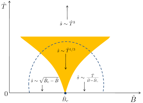
Figure 1: Schematic phase diagram illustrating the various behaviors of the entropy density versus temperature and magnetic field. The region inside the dotted line is controlled by the quantum critical point at $(\hat{T}=0,\hat{B}=\hat{B}_{c})$, and the entropy density can be expressed in terms of a single scaling function $f$ of $(\hat{B}-\hat{B}_{c})/T^{2/3}$. We move around inside this region by changing the temperature $\hat{T}$ and the relevant coupling $\hat{B}-\hat{B}_{c}$. The boundary of the region is defined to be where irrelevant operators become important. The yellow region denotes a regime where temperature is the largest energy scale, corresponding to the argument of the scaling function $f$ being small. Outside the yellow region the low temperature behavior of the entropy density, for fixed $\hat{B}$, is either constant or linear in $\hat{T}$, depending on whether the quantum critical point is approached from below or from above $\hat{B}_{c}$ as $\hat{T}\rightarrow 0$.

1. Our main result is that a continuous quantum phase transition occurs at

   $$\hat{B}_{c}=0.4994240~{}\pm~{}0.0000007$$ (1.2)

2. For $\hat{B}>\hat{B}_{c}$, the entropy density goes to zero linearly with temperature, $\hat{s}\sim\hat{T}$, reflecting the same Fermi liquid physics that was seen in the large $\hat{B}$ limit. Here, however, the linear behavior is occurring at finite charge density where the result does not follow from conformal invariance. Note that the specific heat $C$, at constant $\hat{B}$, has the same behavior as the entropy density, since $C=\hat{T}\partial\hat{s}/\partial\hat{T}\sim\hat{T}$.

3. On approaching $\hat{B}_{c}$ from the large $\hat{B}$ side, the coefficient of the linear term in the $\hat{s}$ versus $\hat{T}$ relation is found to diverge according to,

   $${\hat{s}\over\hat{T}}\sim{1\over(\hat{B}-\hat{B}_{c})^{\sigma}}\hskip 72.26999pt\sigma=1.003~{}\pm~{}0.005$$ (1.3)

   This signals a breakdown of Fermi liquid behavior.

4. Approaching the quantum critical point along the temperature axis at fixed $\hat{B}=\hat{B}_{c}$, the entropy density exhibits a new power law scaling,

   $$\hat{s}\sim\hat{T}^{\alpha}\hskip 72.26999pt\alpha=0.335~{}\pm~{}0.005$$ (1.4)

5. For $\hat{B}<\hat{B}_{c}$ the zero temperature entropy density is found to be nonzero. Near $\hat{B}_{c}$ it obeys the scaling,

   $$\hat{s}\sim(\hat{B}_{c}-\hat{B}_{c})^{\tau}\hskip 72.26999pt\tau=0.500~{}\pm~{}0.001$$ (1.5)

6. The entropy density in the vicinity of the fixed point can be expressed in terms of a scaling function $f$ as,

   $$\hat{s}=\hat{T}^{1/3}f\left({\hat{B}-\hat{B}_{c}\over\hat{T}^{2/3}}\right)$$ (1.6)

   This is to be contrasted with regions far from the critical point, where the entropy density is a nontrivial function of two dimensionless combinations of $\hat{\rho}$, $\hat{B}$ and $\hat{T}$.

From our results, we can infer that the quantum critical theory lives in $1+1$ spacetime dimensions (that is, there are no long range correlations in the remaining 2 spatial directions along the boundary), has dynamical critical exponent $z=3$ (since the value found numerically for $\alpha$ is consistent with $\alpha=1/3$), and has a relevant operator with scaling dimension $2$. The relevant operator corresponds to a change of $\hat{B}$ away from $\hat{B}_{c}$.

1.2 Comparison with known quantum critical systems

It is illuminating to place these results within the context of known quantum critical systems. Although thermodynamic quantities such as the specific heat and magnetization behave in a non-analytic fashion across the phase transition, we note that there is no change of symmetry associated with the transition. A finite temperature example of such behavior is the liquid-gas transition in water. A zero temperature version is a metamagnetic quantum critical point [14, 15], whose behavior closely parallels our system (a finite temperature version of a holographic metamagnetic phase transition in the D4-D8 system was studied in [16]). Metamagnetism refers to a sharp change in the magnetization of a material as an external magnetic field is tuned through some nonzero value. At finite temperature, metamagnetic transitions typically consist of first order lines terminating at a second order critical point, as in the liquid-vapor case. If the critical point can be brought to zero temperature by adjusting some control parameter, one obtains a metamagnetic quantum critical point.

The standard approach to such a quantum critical point is based on the Hertz/Millis theory [17, 18, 19], for which the effective action in momentum space is,

$$S=\int\!d\omega d^{d}k\left({|\omega|\over|k|}+k^{2}+(\hat{B}-\hat{B}_{c})\right)|\phi(\omega,k)|^{2}+\cdots$$ (1.7)

The real bosonic field $\phi$ represents the local magnetization, and the above action can be obtained by integrating out fermions at 1-loop. Under scale transformations acting as $k\rightarrow\lambda k$, we see that $\omega$ should be assigned scale dimension 3, and hence $z=3$. Similarly, $\hat{B}-\hat{B}_{c}$ has scale dimensions $2$. These assignments match what we found for our system, which furthermore corresponds to $d=1$, since the Landau level quantization only allows low energy modes to propagate parallel to $B$.

The action (1.7) is only meant to be applied for $\hat{B}>\hat{B}_{c}$. Indeed, the behavior of our system in the region $\hat{B}<\hat{B}_{c}$, with its nonzero ground state entropy density, cannot be described by this action alone.

Metamagnetic quantum criticality in the compound Sr₃Ru₂O₇ has been the subject of extensive experimental investigation in the past few years (see [15] and references therein), and we will comment on this connection in Section 3.8.

A large number of other AdS/CFT examples undergoing phase transitions have been studied in the literature, both continuous and discontinuous, and at finite and zero temperature; for example [20, 21, 22, 23, 24, 25, 26, 27, 28]. However, our setup seems particularly attractive and is nicely related to real experimental systems. In particular, unlike other examples of quantum phase transitions we do not have to add any extra ingredients in the way of scalar fields or probe branes. We employ only a metric and an Abelian gauge field, with an Einstein-Maxwell-Chern-Simons action that is known to describe all supersymmetric AdS₅ theories related by compactification of Type IIB or M-theory [1, 2, 3]. Thus our framework is both simple and universal.

The remainder of this paper is organized as follows. In Section 2, we spell out the set-up of the holographic calculations, including the specification of initial data at the horizon, asymptotic data at the $AdS_{5}$ boundary, and the construction of regular gauge choices. In Section 3, we present the results of high-precision numerical solutions to the reduced Einstein-Maxwell-Chern-Simons equations, identify the quantum critical point, and critical behavior in its vicinity. We also compare our results with those from the effective Hertz/Millis theory, and comment on the connection with metamagnetic quantum criticality observed in real materials like Sr₃Ru₂O₇. A discussion of the results and open avenues for future research is given in Section 4.

2 Holographic calculations

In this section we spell out some of the technical details of our computations. Results of the numerical calculations will be presented in section 3, and the impatient reader may wish to jump there.

The starting point for our holographic calculations is 5-dimensional Einstein-Maxwell theory with a Chern-Simons term. Throughout this paper, the Chern-Simons coefficient $k$ will be considered fixed at its supersymmetric value $k=2/\sqrt{3}$. A detailed discussion of the action, including boundary terms needed for holographic renormalization, and the construction of the boundary current and stress tensor may be found in [11]. Here, we shall limit our discussion to the field equations and the asymptotic behavior of the fields near the horizon, and at the asymptotic $AdS_{5}$ boundary. The Einstein-Maxwell field equations are given by $dF=0$ and,

$$0 = d*F+kF\wedge F$$

$$R_{MN} = 4g_{MN}+{1\over 3}F^{PQ}F_{PQ}~{}g_{MN}-2F_{MP}F_{N}{}^{P}$$ (2.1)

Uniformity and constancy in time of the magnetic field $B$ and the charge density $\rho$ allow us to restrict to a space-time translation invariant Ansatz, given by,

$$F = Edr\wedge dt+Bdx_{1}\wedge dx_{2}+Pdx_{3}\wedge dr$$

$$ds^{2} = U^{-1}dr^{2}-Udt^{2}+e^{2V}\left(dx_{1}^{2}+dx_{2}^{2}\right)+e^{2W}\left(dx_{3}+Cdt\right)^{2}$$ (2.2)

The functions $E,P,U,V,W,C$ depend only on the radial coordinate $r$, while the magnetic field $B$ is constant by the Bianchi identity. A gauge choice has been made here for the coordinate $r$ in order to put the Ansatz in canonical form with matching coefficients of its first two terms in $ds^{2}$. The reduced field equations were given in [11].

2.1 Data at the horizon

The reduced field equations are to be solved subject to regularity conditions at the horizon and at the asymptotic $AdS_{5}$ boundary $r=\infty$. For the purpose of numerical analysis, it will be convenient to parametrize solutions in terms of data at the horizon which satisfy the regularity conditions at the horizon. Regularity of the full solution, including at the asymptotic $AdS_{5}$ boundary, must then be verified numerically for each set of data.

We begin by spelling out the data at the horizon. (This discussion will parallel the one presented in [11], but there will be important differences motivated by the need to remedy the gauge choice problems alluded to in the Introduction.) The (outer) horizon at $r=r_{+}$, and the Hawking temperature $T$ are defined by,

$$U(r_{+})=0\hskip 72.26999pt4\pi T=U^{\prime}(r_{+})$$ (2.3)

Our numerical analysis will always be carried out at $T\not=0$, even though $T$ may become very small; thus, we are free to rescale $t$, and set $U^{\prime}(r_{+})=1$. By rescaling also $x_{1},x_{2},x_{3}$, we may set $V(r_{+})=W(r_{+})=0$. Invariance of the Ansatz under $\alpha$-symmetry, (under which $x_{3}\to x_{3}-\alpha t$, $C\to C+\alpha$, and $E\to E-\alpha P$), allows us to set $C(r_{+})=0$. With these choices, the fields at the horizon take the form,

$$F_{H} = q\,dr\wedge dt+b\,dx_{1}\wedge dx_{2}+p\,dx_{3}\wedge dr$$

$$ds_{H}^{2} = dx_{1}^{2}+dx_{2}^{2}+dx_{3}^{2}$$ (2.4)

The reduced field equations of [11] for $E,P,U,V,W,C$, combined with the requirement of regularity at the horizon, dictate certain relations amongst the remaining data at the horizon, namely $q,b,p,V^{\prime}(r_{+})$, $W^{\prime}(r_{+})$, and $C^{\prime}(r_{+})$. They are given by (for $U^{\prime}(r_{+})=1$),

$$0 = p-q\left(C^{\prime}(r_{+})-2kb\right)$$

$$3V^{\prime}(r_{+}) = 12-2q^{2}-4b^{2}$$

$$6W^{\prime}(r_{+}) = 24-4(q^{2}-b^{2})-3C^{\prime}(r_{+})^{2}$$ (2.5)

Given $(b,q)$, the data $p$ and $C^{\prime}(r_{+})$ are related to one another by the first equation of (2.1). Keeping either $p$ or $C^{\prime}(r_{+})$ as an independent free parameter, the remaining initial data $V^{\prime}(r_{+})$ and $W^{\prime}(r_{+})$ are uniquely determined by the last two equations of (2.1).

2.2 Gauge fixing and regularity

The parametrization of the horizon data presented above is more general than the one given in [11], since here the parameter $p$ is kept unspecified, while $p$ was set to 0 in [11]. The argument invoked to set $p=0$ was the covariance of the Ansatz of (2) under boosts in the $x_{3}$-direction. Under a boost by velocity $\beta$, the space-time coordinates transform as usual, $t\to\tilde{t}=\gamma(t-\beta x_{3})$ and $x_{3}\to\tilde{x}_{3}=\gamma(x_{3}-\beta t)$ with $\gamma^{2}(1-\beta^{2})=1$, and where $\beta$ cannot exceed the speed of light, $|\beta|<1$. The transformation under boosts of the functions $(E,P,U,V,W,C)\to(\tilde{E},\tilde{P},\tilde{U},\tilde{V},\tilde{W},\tilde{C})$, however, must be accompanied by a transformation of the holographic coordinate $r\to\tilde{r}$, which is required to restore the boosted Ansatz back to the canonical form of (2). As a result, the Maxwell fields transform as follows,

$$\tilde{E}(\tilde{r})d\tilde{r} = \gamma\Big{(}E(r)-\beta P(r)\Big{)}dr$$

$$\tilde{P}(\tilde{r})d\tilde{r} = \gamma\Big{(}P(r)-\beta E(r)\Big{)}dr$$ (2.6)

where $\tilde{U}(\tilde{r})^{-1}d\tilde{r}=U(r)^{-1}dr$. The ratio $p/q$ transforms as $\tilde{p}/\tilde{q}=(p/q-\beta)/(1-\beta p/q)$. Clearly, provided $q^{2}>p^{2}$, a boost by $\beta=p/q$ may be used to set $\tilde{p}$ to zero. The problem, however, is that the coordinate transformation $r\to\tilde{r}$ required to accompany this boost may be singular on some of the functions $E,P,U,V,W,C$. For example, the transformation law under a boost by velocity $\beta$ of the function $C$ is given by,

$$C(r)\to\tilde{C}(\tilde{r})={(C(r)+\beta)(1+\beta C(r))e^{2W(r)}-\beta U(r)\over(1+\beta C(r))^{2}e^{2W(r)}-\beta^{2}U(r)}$$ (2.7)

We have verified numerically that, in the region of low $T$ where our numerics were found to break down in [11], the denominator in (2.7) indeed crosses zero as $r$ is increased away from the horizon at $r_{+}$, thereby rendering this boost transformation singular.

The remedy to this problem is simple: the parameter $p$ should be left unspecified, thereby eliminating the need to perform boost transformations on the fields. It will be convenient to parametrize solutions by the values $b,q,C^{\prime}(r_{+})$, so that the remaining initial data at the horizon, $p,V^{\prime}(r_{+})$, and $W^{\prime}(r_{+})$ are uniquely determined by (2.1). Not every assignment of $b,q,C^{\prime}(r_{+})$ will produce a regular solution. Also, two regular solutions may be related to one another by a regular boost, and thus be physically equivalent. The parameter space of all regular solutions may be described as follows. To every pair $(b,q)$ we assign the maximal interval $\Gamma(b,q)$ on the real line such that for every value of $C^{\prime}(r_{+})\in\Gamma(b,q)$, the solution specified by the parameters $b,q,C^{\prime}(r_{+})$ is regular. The end points of the interval $\Gamma(b,q)$ correspond to the limits where the velocity of the solution tends to the speed of light. When computing boost invariant physical quantities, such as the magnetic field $B$, and the rest frame temperature $T$, charge density $\rho$, and entropy density $s$, the datum $C^{\prime}(r_{+})$ may be chosen to be any value in the interval $\Gamma(b,q)$.

2.3 Data at the asymptotic $AdS_{5}$ boundary $r\to\infty$

For regular solutions the functions $U,V,W,E,P,C$ have the following asymptotic behavior as $r\to\infty$, (keeping only leading contributions),

$$U\sim r^{2}\hskip 61.42993pt \qquad e^{2V}\sim vr^{2} \qquad e^{2W}\sim wr^{2}$$

$$E\sim(e_{3}-c_{0}p_{3})r^{-3} \qquad P\sim p_{3}r^{-3} \qquad C\sim c_{0}$$ (2.8)

In these coordinates, the conformal boundary metric is $-dt^{2}+v(dx_{1}^{2}+dx_{2}^{2})+w(dx_{3}+c_{0}dt)^{2}$, and the solution’s velocity is $\sqrt{w}~{}c_{0}$. Rescaling $x_{1},x_{2}$ by $\sqrt{v}$, and $x_{3}$ by $\sqrt{w}$, while combining an $\alpha$-transformation with a boost by a velocity $\beta=-\sqrt{w}c_{0}$, restores the coordinates to the standard Minkowski metric, and yields the following expressions for the physical magnetic field $B$, temperature $T$, charge density $\rho$, and entropy density $s$ in the rest frame of the solution, (see [11] for derivations),

$$B={b\over v}\hskip 43.36243ptT={\gamma_{c}\over 4\pi}\hskip 43.36243pt\rho=\gamma_{c}(e_{3}-c_{0}p_{3})\hskip 43.36243pts={1\over 4v\gamma_{c}\sqrt{w}}$$ (2.9)

Here, $\gamma_{c}^{2}=(1-wc_{0}^{2})^{-1}$, and the normalized entropy density $s$ is defined as $s=G_{5}S/{\rm Vol}$, where $S$ is the total entropy in volume Vol, and $G_{5}$ is the 5-dimensional Newton constant.

By virtue of scale invariance, only dimensionless combinations of quantities, such as $B^{3}/\rho^{2}$, afford any intrinsic physical meaning. Thus, the results on phase transitions and associated critical exponents at critical points, aimed for in this paper, will all be derived by evaluating the dependence between the dimensionless physical quantities $\hat{s}$ and $\hat{T}$, for various (fixed) values of $\hat{B}$, which were all defined in (1.1).

2.4 Numerical fine points

The initial data for any regular solution is a pair $(b,q)$ and a value $C^{\prime}(r_{+})\in\Gamma(b,q)$, where the interval $\Gamma(b,q)$ was defined so that the data $b,q,C^{\prime}(r_{+})$ produce a regular solution. For certain values of $(b,q)$, the interval $\Gamma(b,q)$ may be empty. For $k=2/\sqrt{3}$, numerical analysis yields the following bound,

$$\Gamma(b,q)=\emptyset\hskip 57.81621pt{\rm when}\quad q^{2}+2b^{2}>6$$ (2.10)

The precise form of the critical curve ${\cal C}$ in the $(b,q)$-plane inside of which $\Gamma(b,q)\not=\emptyset$ is not known analytically, but may be obtained numerically, as was done in [11].

Away from the low temperature regime the interval $\Gamma(b,q)$ is sufficiently large that it is possible, at least for $k=2/\sqrt{3}$, to make a single uniform choice for $C^{\prime}(r_{+})$ and still cover most of the parameter space. A convenient choice is $C^{\prime}(r_{+})=2b$. However, as the temperature is lowered $\Gamma(b,q)$ shrinks, and one is forced to tune $C^{\prime}(r_{+})$ to greater precision. This effect becomes especially pronounced in the region of low magnetic field where a ground state entropy develops. However, by specifying more general tunings for $C^{\prime}(r_{+})$ as we vary $(b,q)$ we are able to fully cover the low temperature region.

The approach to ultra-low temperatures, which is needed in various parts of our numerical work, requires a high degree of fine-tuning of the horizon initial data $(b,q)$ and the gauge choice $C^{\prime}(r_{+})$. It also requires evaluating the asymptotic data, such as $v,w,c_{0},e_{3}$ and $p_{3}$ at large values of $r$, which we typically have taken to range from $10^{15}$ to $10^{20}$. With such high degrees of fine-tuning, and extended ranges of integration, the issue of numerical accuracy and numerical stability of the calculations becomes of utmost importance. Our calculations were performed with 15 to 20 digits accuracy, and the ODEs were solved with absolute and relative error tolerances ranging from $10^{-10}$ to $10^{-13}$ for the lowest temperatures. Stability of the results was checked versus changing the asymptotic value of $r$, the absolute and relative error tolerances, and the number of digits.

3 Numerical results

In this section, we present our numerical results, organized as a function of the magnitude of the magnetic field $\hat{B}$, starting at large $\hat{B}$.

3.1 Large $\hat{B}$ regime

In [11] the case $\hat{B}\approx.53$ (quoted there as $\hat{B}^{3}\approx.15$) was studied at the supersymmetric value $k=2/\sqrt{3}$. As displayed in Figure 3 of [11] the low temperature entropy density was seen to drop well below its $\hat{B}=0$ value, and appeared to be heading towards zero. However, the numerics broke down at temperature $\hat{T}\approx.02$, and so did not allow for an exploration of ultra-low temperatures. By adjusting $C^{\prime}(r_{+})$ as we lower the temperature, we can do much better, as shown in Figure 2 below. The entropy density clearly vanishes at zero temperature. A linear behavior, $\hat{s}\sim\hat{T}$ is evident in the approach to zero temperature, as shown in the right panel of Figure 2.

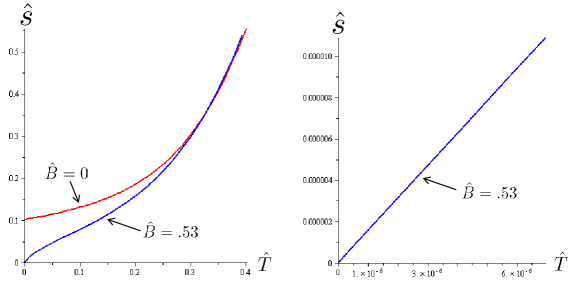
Figure 2: Plot of entropy versus temperature. On the left we compare $\hat{B}=.53$ to $\hat{B}=0$; this plot is an improved version of Fig. 3 in [11]. On the right we exhibit the linear $\hat{s}\sim\hat{T}$ low temperature behavior.

By repeating this analysis for other sufficiently large values of $\hat{B}$, we find similar behavior: the entropy density vanishes at zero temperature, and does so linearly at very low temperatures. This linear behavior is characteristic of Fermi liquids. The textbook intuitive explanation for the linear dependence is that at low temperature the smoothed out step function form of the Fermi-Dirac distribution implies that only electrons within energy $k_{B}T$ of the Fermi energy contribute. We indeed expect our system to be described by a theory of light fermions in this large $\hat{B}$, low $\hat{T}$ regime, since the magnetic field raises up all energies except for the lowest fermion Landau level. Our numerical results are a pleasing confirmation of this intuition.

In the $\hat{B}\rightarrow\infty$ limit it was found in [10] that a near horizon AdS${}_{3}\times\bf R^{2}$ factor emerged at low energies, and the resulting $1+1$ dimensional conformal invariance could be used to explain the $\hat{s}\sim\hat{T}$ behavior. This is no longer true away from this limit, as the charge density $\rho$ introduces an additional scale into the problem, and from the numerics we can see that the near horizon geometry becomes deformed away from AdS${}_{3}\times\bf R^{2}$.

Charged black hole solutions involving scalar fields whose entropy densities similarly go to zero at extremality have been studied in [29, 30, 31, 32].

3.2 Approaching $\hat{B}_{c}$

Experimentally, a breakdown of Fermi liquid behavior upon tuning an external magnetic field can often be seen in a divergence of the specific heat coefficient, defined as,

$$\gamma={C\over\hat{T}}$$ (3.1)

Since $C=\hat{T}{\partial\hat{s}/\partial\hat{T}}$, we can equivalently write $\gamma=\hat{s}/\hat{T}$ at low temperatures. In our system, $\gamma$ stabilizes at a constant value for large $\hat{B}$, but is seen to diverge at a critical value $\hat{B}=\hat{B}_{c}$. Numerically, the critical value $\hat{B}_{c}$ is found to be bounded as follows,

$$0.124568<\hat{B}_{c}^{3}<0.124569$$ (3.2)

which results in the the value quoted already in (1.2), namely $\hat{B}_{c}=0.4994240\,\pm\,0.0000007$. To characterize the divergence we display a plot of $\hat{s}/\hat{T}$ versus $1/(\hat{B}-\hat{B}_{c})$, as $\hat{T}\to 0$ in Figure 3. The straight line shows that the low temperature entropy behaves as

$${\hat{s}\over\hat{T}}\sim{1\over\hat{B}-\hat{B}_{c}}$$ (3.3)

as $\hat{T}\rightarrow 0$ for fixed $\hat{B}$ near (but larger than) $\hat{B}_{c}$. Upon approaching $\hat{B}_{c}$ we find that the linear regime with $\hat{s}\sim\hat{T}$ is confined to an ever smaller low temperature window.

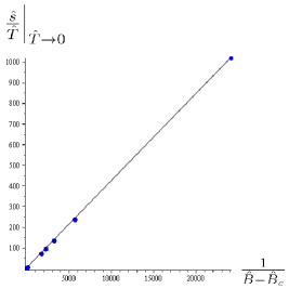
Figure 3: Plot showing the divergence of $\hat{s}/\hat{T}$ near $\hat{B}_{c}$ at low temperatures. The straight line through the data points is included to guide the eye.

3.3 Scaling at the critical magnetic field $\hat{B}=\hat{B}_{c}$

Next we set $\hat{B}=\hat{B}_{c}$ and again study the low temperature behavior of the entropy density. We find a new scaling law, $\hat{s}\sim\hat{T}^{1/3}$, which numerically extends over at least four orders of magnitude in temperature, $10^{-8}<T<6\times 10^{-3}$, as shown in Figures 4. This nontrivial power law manifestly represents non-Fermi liquid behavior, analogous to what is seen in real materials at a quantum critical point.

Towards ultra-low temperatures, the numerical behavior of $\hat{s}$ will ultimately turn over to be linear in $\hat{T}$ (for $\hat{B}>\hat{B}_{c}$) or to be a non-zero constant for $\hat{B}<\hat{B}_{c}$ (see the next subsection). This deviation from $\hat{s}\sim\hat{T}^{1/3}$ scaling is caused by the fact that the value of $\hat{B}_{c}$ is known only numerically from (1.2), and we are never able to sit at precisely the value of $\hat{B}$.

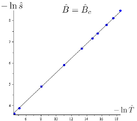
Figure 4: Plot showing $\hat{s}\sim\hat{T}^{1/3}$ scaling behavior at $\hat{B}=\hat{B}_{c}$. The straight line through the data points is included to guide the eye, and has slope $1/3$, consistent with (1.4).

3.4 The quantum critical region and crossover

The $\hat{s}\sim\hat{T}^{1/3}$ scaling law extends to the vicinity of the critical magnetic field $\hat{B}_{c}$, but the range over which this scaling law holds shrinks as $|\hat{B}-\hat{B}_{c}|$ is increased. The corresponding behavior of $\hat{s}$ is illustrated in Figure 5.

First, on the right panel of Figure 5, $-\ln(\hat{s})$ is plotted versus $-\ln(\hat{T})$ for $\hat{B}^{3}=0.124569$. The $\hat{T}^{1/3}$ scaling law exhibited in the preceding subsection, is clearly recovered here. At sufficiently high temperature, the $\hat{T}^{1/3}$ behavior eventually crosses over to the $\hat{T}^{3}$ dependence controlled by the UV theory. This is clearly shown on the right panel of Figure 5, where the cross-over region may be identified with the temperature interval $0.02<T_{\rm cross-over}<0.5$.

Second, on the left panel of Figure 5, the flows of $-\ln(\hat{s})$ as a function of $-\ln(\hat{T})$ at various fixed values of $\hat{B}$ are shown. Curves a, b, c, d, e, and f clearly exhibit the turnover from $\hat{s}\sim\hat{T}^{1/3}$ scaling behavior to linear $\hat{s}\sim\hat{T}$ behavior at ultra-low temperatures. Given this cross-over behavior, we know that the corresponding values of $\hat{B}$ must all be above the critical magnetic field $\hat{B}_{c}$, with value closest to critical corresponding to curve f with $\hat{B}^{3}=0.124569$. Curve g behaves completely differently at ultra-low temperatures, and $\hat{s}$ is seen to tend towards a non-zero constant. Given this behavior, we know that the corresponding value of $\hat{B}$ must be below critical. Combining both results gives $0.124568<\hat{B}_{c}^{3}<0.124569$, as announced in (3.2), and (1.2).

Finally, as $\hat{B}-\hat{B}_{c}$ is increased, the region over which the $\hat{s}\sim\hat{T}^{1/3}$ scaling law holds becomes smaller and smaller, being overtaken by the $\hat{s}\sim\hat{T}^{3}$ law at high $\hat{T}$ joining the $\hat{s}\sim\hat{T}$ law at low $\hat{T}$, and ultimately will have disappeared altogether by the time $\hat{B}^{3}=0.2$ is reached (this result is not shown in the figures).

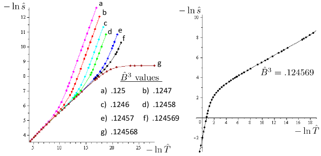
Figure 5: The left plot shows the crossover of $\hat{s}$ for low $\hat{T}$. At moderately low temperatures $\hat{s}$ scales as $\hat{T}^{1/3}$ (lower left corner of the plot), while at ultra-low temperatures $\hat{s}$ scales as $\hat{T}$ for $\hat{B}>\hat{B}_{c}$ (curves a, b, c, d, e, f), and tends to a non-zero constant for $\hat{B}<\hat{B}_{c}$ (curve g). The right plot shows the crossover for $\hat{s}$ from the moderately low temperature $\hat{T}^{1/3}$ scaling to the high temperature $\hat{T}^{3}$ behavior. The dots represent numerical data points, while the solid interpolating lines are included to guide the eye.

3.5 Low $\hat{B}$ region

Decreasing the magnetic field further, namely $\hat{B}<\hat{B}_{c}$, we find a completely different low temperature behavior: the entropy now stabilizes to a nonzero value at $\hat{T}=0$. We plot this limiting value in Figure 6. In [11] we speculated that an infinitesimally small magnetic field might be sufficient to remove the ground state entropy of the $\hat{B}=0$ solution. We now see that this speculation is incorrect – only magnetic fields $\hat{B}\geq\hat{B}_{c}$ accomplish this.

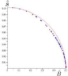
Figure 6: Extremal entropy density: blue points represent results for the entropy density at very low temperatures in the region $\hat{B}<\hat{B}_{c}$. The red curve is a plot of the function ${1\over 4\sqrt{6}}\sqrt{1-\left({\hat{B}\over\hat{B}_{c}}\right)^{2}}$

The extremal entropy turns on continuously below the critical magnetic field. A curve that passes through all the points to better than $.5\%$ accuracy is given by

$$\hat{s}={1\over 4\sqrt{6}}{\sqrt{1-\left({\hat{B}\over\hat{B}_{c}}\right)^{2}}\over(1+\hat{B}^{2})^{7/4}}$$ (3.4)

The prefactor of $1/(4\sqrt{6})$ is fixed by the value for the purely electrically charged black brane, which is of course known analytically. It is remarkable that this function fits the data so well, but we are unable to say whether it represents an exact analytical result.

To excellent accuracy, and as exhibited by (3.4), we find

$$\hat{s}\sim\sqrt{\hat{B}_{c}-\hat{B}}$$ (3.5)

near the critical point. If we increase the temperature at fixed magnetic field in this regime, we again find a region obeying the same $\hat{s}\sim\hat{T}^{1/3}$ scaling as described in section 3.3.

3.6 Scaling region near the critical point

The fact that the entropy density at the critical magnetic field has a simple power law dependence on temperature is indicative of a quantum critical point. Recall that since we are working in terms of dimensionless quantities as defined by the scalings in the asymptotically AdS₅ region, a priori the dimensionless entropy density $\hat{s}$ is allowed to be an arbitrary function of the dimensionless temperature $\hat{T}$. This interpretation can be sharpened further by writing down a scaling form for the entropy in the vicinity of the critical point

$$\hat{s}=\hat{T}^{1\over 3}f\left({\hat{B}-\hat{B}_{c}\over\hat{T}^{2/3}}\right)$$ (3.6)

where, according to our results, the scaling function $f(x)$ has asymptotic behavior

$$f(x)\sim\left\{\begin{array}[]{ccc}c_{1}\sqrt{-x}&&x\rightarrow-\infty\\ c_{2}&&x\rightarrow 0\\ {c_{3}/x}&&x\rightarrow\infty\end{array}\right.$$ (3.10)

for some constants $c_{1,2,3}$. In general, the entropy is a function of two dimensionless combinations of $B$, $\rho$, and $T$, whereas near the critical point the claim is that it can be written as a function of only one variable. All of this is of course standard from the general theory of classical and quantum critical phenomena.

It is further useful to recall that for a quantum critical theory in $d$ spatial dimensions, with dynamical critical exponent $z$, and with a relevant coupling $m$ of scale dimension $\Delta$, the entropy density will take the scaling form

$$s=T^{d/z}f\left({m^{2/\Delta}\over T^{2/z}}\right)$$ (3.11)

Comparing to (3.10) we read off $d=1$, $z=3$, and $\Delta=2$.

We have verified that the scaling form (3.10) conforms to our numerical results near the critical point at $\hat{B}=\hat{B}_{c}$ and $\hat{T}=0$. From the numerics we can reconstruct the form of the scaling function, which is shown in Figure 7.

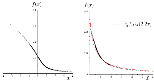
Figure 7: Plots of the scaling function $f(x)$ controlling the thermodynamics within the scaling region. On the right plot we restrict to $x>0$, corresponding to $\hat{B}>\hat{B}_{c}$, and compare the scaling function from gravity with a free field computation based on the Hertz/Millis theory; the latter is displayed as a red line. The factors of $1/10$ and $2.2$ in the latter are chosen to give a good match, and are expected since the the gravitational result contains a factor of Newton’s constant and the normalizations of the magnetic fields need not agree.

We can use this to determine the constants appearing in (3.10) to be,

$$c_{1}\approx 0.172\hskip 72.26999ptc_{2}\approx 0.110\hskip 72.26999ptc_{3}\approx 0.045$$ (3.12)

As noted in the Introduction, the standard approach to modelling a magnetically tuned quantum critical point of the type that we are seeing is based on the Hertz/Millis theory. We consider the action in (1.7) with $d=1$. To the extent that this action captures the low energy degrees of freedom of our theory, it is natural to compute its finite temperature entropy density and compare to our results. This cannot be entirely correct for a number of reasons, not least that there is no way of explaining the ground state entropy density in this framework, but the comparison is instructive nonetheless. In the free field limit we just need the dispersion relation implied by (1.7), which is

$$\omega=|k|(k^{2}+m^{2})\hskip 86.72377ptm^{2}=\hat{B}-\hat{B}_{c}$$ (3.13)

The partition function is

$$\ln Z=-{L\over 2\pi}\int_{-\infty}^{\infty}\!dk\ln(1-e^{-\beta|k|(k^{2}+m^{2})})$$ (3.14)

from which we can extract the entropy density as

$$s={1\over L}\left(1-\beta{\partial\over\partial\beta}\right)\ln Z$$ (3.15)

We can write the result in a scaling form as

$$s=T^{1/3}f_{HM}\left({\hat{B}-\hat{B}_{c}\over T^{2/3}}\right)$$ (3.16)

and then compare with the scaling function coming from gravity. The comparison is shown in the right panel of Figure 7. We only compare in the region $\hat{B}>\hat{B}_{c}$, since it is only in this region that the Hertz/Millis action applies. Nothing fixes the normalization of the magnetic field appearing in (1.7) compared to that in gravity, and so we have allowed ourselves to adjust this relationship to achieve a good fit. Similarly, we have introduced a parameter to adjust the overall normalizations. The functions match surprisingly well, although it is unclear how much significance to attach to this.

3.7 The quantum critical point

Initial data yielding our closest approach to the quantum critical point is given by

$$b = 1.7320507$$

$$q = 5.08\times 10^{-4}$$ (3.17)

This choice of $(b,q)$ along with the gauge choice $C^{\prime}(r_{+})=3.464063$ leads to the following values for the asymptotic parameters of (2.3),

$$v = 5.23811\times 10^{-14},\hskip 21.68121ptw=1.60044\times 10^{-9}\hskip 21.68121ptc_{0}=859.258$$

$$e_{3} = 5.20520\times 10^{20}\hskip 31.07556ptp_{3}=-2.08236\times 10^{16}$$ (3.18)

from which we can compute the temperature and entropy density as

$$\hat{T} = 9.59602\times 10^{-9}$$

$$\hat{s} = 2.08699\times 10^{-4}$$ (3.19)

From (3.17) we see that there is a large hierarchy between the size of the electric and magnetic charges at the horizon in our chosen coordinates. Nevertheless, measured at infinity in the rest frame the ratio of these quantities is of order unity, $\hat{B}_{c}^{3}\approx 0.124569$. This happens because there are large rescalings that occur in the process of integrating out from the horizon to the asymptotic regions, as illustrated by the magnitude of the parameters in (3.18). Using (2.9) these can convert a large hierarchy into one of order unity.

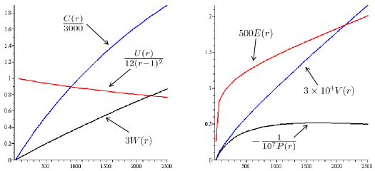
Figure 8: Plots of the metric functions for a solution very near the quantum critical point. Multiplicative factors have been included to allow the functions to appear on the same plot. The form of the functions near the horizon show that the metric is behaving as AdS${}_{3}\times{\bf R}^{2}$ plus small corrections. These small corrections are amplified in passing to the asymptotic AdS₅ regime.

It is instructive to examine the metric functions for this near critical solution. In Figure 8 we provide plots of these functions in the near (and not so near) horizon region. Near the horizon, one can think of these metric functions as representing a deformation of the configuration

$$U(r) = 12(r-1)^{2}\hskip 75.88371ptB=\sqrt{3}$$

$$C(r) = 2\sqrt{3}(r-1)\hskip 72.26999ptV=W=E=P=0$$ (3.20)

This represents AdS${}_{3}\times\bf R^{2}$ in “boosted coordinates” with magnetic flux. We expect that, as we get nearer and nearer to the critical point, the metric functions will approach (3.20) to greater and greater accuracy. On the other hand, it is crucial that there always be some deviation away from (3.20), as this solution is purely magnetic with vanishing electric charge density. Presumably what happens is that there is a fine-tuned limit in which all of the charge is carried by the bulk supergravity fields outside the near horizon region; this is possible by virtue of the Chern-Simons term. It would of course be extremely useful if this limiting solution could be found analytically.

We close this subsection with an issue which has not yet been conclusively resolved by our numerical studies. For large $\hat{B}$, all flows towards lower $\hat{T}$ end in the purely magnetic fixed point solution of [10], whose near-horizon geometry is $AdS_{3}\times{\bf R}^{2}$. More precisely, it can be shown numerically that all flows for $\hat{B}>\hat{B}_{c}$ end up at the purely magnetic fixed point. Where do the flows for $\hat{B}<\hat{B}_{c}$ end? Numerically, we have established that flows for $\hat{B}$ less than but close to $\hat{B}_{c}$ come near the purely magnetic fixed point, but at temperatures so low (on the order of $\hat{T}\sim 10^{-15}$) that further numerical analysis can be pursued only at the cost of calculation times and memory which exceed those of our computers. Thus, the logical possibility that the flows with $\hat{B}<\hat{B}_{c}$ end up on the critical curve, before the purely magnetic fixed point has been attained, cannot be excluded at this time. If this situation is in fact the one that occurs, then it would have a surprising similarity to the dynamics of the $k=1$ theory, derived in [11].

3.8 Metamagnetic quantum criticality in Sr₃Ru₂O₇

We close this section with a few words about a real system that parallels ours in a number of ways. Quantum criticality and novel phases in Sr₃Ru₂O₇ have been the subject of much experimental and theoretical interest in the past few years; e.g. [15, 34]. Sr₃Ru₂O₇ is a layered structure, which for a large magnetic field perpendicular to the layers exhibits a line of first order metamagnetic phase transitions at finite temperature, ending at a finite temperature critical point. By including a component of magnetic field in the plane of the layers, the critical point can be brought to zero temperature. As in our case, the transition occurs at finite magnetic field, and involves no change of symmetry. Away from the critical point the system behaves as a Fermi liquid, with entropy density linear in temperature. As the critical point is approached, the linear term diverges as $s/T\sim 1/(B-B_{c})$, just as we found (in this case $B_{c}$ is approximately $8$ Tesla.) In recent work, the complete “entropy landscape” of Sr₃Ru₂O₇ at finite temperature and magnetic field has been mapped out [15]. In very pure samples, as one tries to sit right on top of the critical point one finds instead that a new phase emerges, which is believed to be a spatially anisotropic nematic phase [33, 34]. This has been described as nature’s solution to the problem of avoiding a finite entropy density at zero temperature. The parallels with our system are evident (though an obvious difference is that our critical theory effectively sees only a single spatial direction, compared to the two in-plane directions in Sr₃Ru₂O₇), and lead us to speculate whether in our case the extremal black hole phase is unstable and gives way to a new phase with reduced symmetry, as in [35].

4 Discussion

We have found a holographic description of a quantum critical point, reached by tuning a magnetic field at finite density, that nicely resembles examples seen in the real world. In particular, approached from the high $B$-field side, we have Fermi liquid behavior; as the magnetic field is lowered the specific heat coefficient diverges, and we enter a regime of non-Fermi liquid behavior with nontrivial scaling properties.

The most exotic property as compared to known physical examples is the existence of a ground state entropy on the low field side of the transition. The presence of a non-vanishing entropy at $T=0$ for $\hat{B}<\hat{B}_{c}$ would again seem to contradict the third “law” of thermodynamics [11], as it did in the absence of magnetic fields. Actually, our results show that the lifting of the ground state entropy as a function of an external magnetic field is a subtle and dynamical issue. Also, we expect the ground state entropy to be lifted by instabilities driving the system towards inhomogeneity, or by turning on further fields besides an external magnetic field.

It is worth emphasizing again the universality of our results: they apply to all supersymmetric AdS₅ examples arising from IIB or M-theory, since all such theories admit a consistent truncation to the Einstein-Maxwell-Chern-Simons theory used here [1, 2, 3]. We did not have to introduce any model building devices in the way of probe branes or scalar fields.

There are many open questions and avenues for further investigation. Many of our numerical results cry out for an analytical derivation. In particular, one would expect to be able to derive the value $z=3$ of the dynamical exponent, and the dimension $\Delta=2$ of the relevant operator governing the critical theory. It may similarly be possible to understand these results microscopically on the gauge theory side.

All of our results were presented for the supersymmetric value of the Chern-Simons coupling, $k=2/\sqrt{3}$, but it would be useful to consider other values as well. Our expectation is that as $k$ is increased the critical point will retain its character but with $\hat{B}_{c}$ moving to a smaller value. An interesting question would then be whether we reach $\hat{B}_{c}=0$ at finite $k$, for if so there would no longer be an extremal black hole phase.

In this work we have only considered the thermodynamics, but the existence of the critical theory implies scaling behavior of correlation functions with respect to frequency and momentum. Computing these would be valuable in pinning down the precise connection to the Hertz/Millis theory.

Finally, to more closely model real systems it would be very interesting to construct a version of our system giving rise to critical behavior in two or three spatial dimensions.

Acknowledgments

It is a pleasure to thank David Berenstein, Sudip Chakravarty, Tom Faulkner, Gary Horowitz, Don Marolf, Eric Perlmutter, Joe Polchinski, and Matt Roberts for helpful discussions.

References

- [1] A. Buchel and J. T. Liu, “Gauged supergravity from type IIB string theory on Y(p,q) manifolds,” Nucl. Phys. B 771 (2007) 93 [arXiv:hep-th/0608002].
- [2] J. P. Gauntlett, E. O Colgain and O. Varela, “Properties of some conformal field theories with M-theory duals,” JHEP 0702 (2007) 049 [arXiv:hep-th/0611219].
- [3] J. P. Gauntlett and O. Varela, “Consistent Kaluza-Klein Reductions for General Supersymmetric AdS Solutions,” Phys. Rev. D 76 (2007) 126007 [arXiv:0707.2315 [hep-th]].
- [4] S. Sachdev, “Quantum Phase Transitions”, Cambridge University Press (2001)
- [5] H. Liu, J. McGreevy and D. Vegh, “Non-Fermi liquids from holography,” arXiv:0903.2477 [hep-th].
- [6] M. Cubrovic, J. Zaanen and K. Schalm, “Fermions and the AdS/CFT correspondence: quantum phase transitions and the emergent Fermi-liquid,” arXiv:0904.1993 [hep-th].
- [7] T. Faulkner, H. Liu, J. McGreevy and D. Vegh, “Emergent quantum criticality, Fermi surfaces, and AdS2,” arXiv:0907.2694 [hep-th].
- [8] T. Faulkner and J. Polchinski, “Semi-Holographic Fermi Liquids,” arXiv:1001.5049 [hep-th].
- [9] S. J. Rey, “String Theory On Thin Semiconductors: Holographic Realization Of Fermi Points And Surfaces,” Prog. Theor. Phys. Suppl. 177, 128 (2009) [arXiv:0911.5295 [hep-th]].
- [10] E. D’Hoker and P. Kraus, “Magnetic Brane Solutions in AdS,” JHEP 0910, 088 (2009) [arXiv:0908.3875 [hep-th]].
- [11] E. D’Hoker and P. Kraus, “Charged Magnetic Brane Solutions in and the fate of the third law of thermodynamics,” arXiv:0911.4518 [hep-th].
- [12] D. Anninos, W. Li, M. Padi, W. Song and A. Strominger, “Warped AdS3 Black Holes,” JHEP 0903, 130 (2009) [arXiv:0807.3040 [hep-th]].
- [13] G. Compere and S. Detournay, “Boundary conditions for spacelike and timelike warped AdS3 spaces in topologically massive gravity,” JHEP 0908, 092 (2009) [arXiv:0906.1243 [hep-th]].
- [14] A. J. Millis, A. J. Schofield, G. G. Lonzarich and S. A. Grigera, “Metamagnetic quantum criticality in metals,” Phys. Rev. Lett. 88, 217204 (2002).
- [15] A. W. Rost, R. S. Perry, J.-F. Mercure, A. P. Mackenzie, and S. A. Grigera “Entropy Landscape of Phase Formation Associated with Quantum Criticality in ”, Science Vol. 325. no. 5946, pp. 1360 - 1363 (2009)
- [16] G. Lifschytz and M. Lippert, “Holographic Magnetic Phase Transition,” Phys. Rev. D 80, 066007 (2009) [arXiv:0906.3892 [hep-th]].
- [17] J. A. Hertz, “Quantum critical phenomena,” Phys. Rev. B 14 1165 (1976).
- [18] A. J. Millis, “Effect of a nonzero temperature on quantum critical points in itinerant fermion systems”, Phys. Rev. B 48, 7183–7196 (1993)
- [19] H. v. Lohneysen, A. Rosch, M. Mojta, and P. Wolfle, “Fermi-liquid instabilities at magnetic quantum phase transitions”, Rev. Mod. Phys. 79 , 1015–1075 (2007)
- [20] E. Witten, “Anti-de Sitter space, thermal phase transition, and confinement in gauge theories,” Adv. Theor. Math. Phys. 2, 505 (1998) [arXiv:hep-th/9803131].
- [21] A. Chamblin, R. Emparan, C. V. Johnson and R. C. Myers, “Charged AdS black holes and catastrophic holography,” Phys. Rev. D 60, 064018 (1999) [arXiv:hep-th/9902170].
- [22] A. Parnachev and D. A. Sahakyan, “Chiral phase transition from string theory,” Phys. Rev. Lett. 97, 111601 (2006) [arXiv:hep-th/0604173].
- [23] D. Mateos, R. C. Myers and R. M. Thomson, “Holographic phase transitions with fundamental matter,” Phys. Rev. Lett. 97, 091601 (2006) [arXiv:hep-th/0605046].
- [24] J. L. Davis, M. Gutperle, P. Kraus and I. Sachs, “Stringy NJL and Gross-Neveu models at finite density and temperature,” JHEP 0710, 049 (2007) [arXiv:0708.0589 [hep-th]].
- [25] S. A. Hartnoll, C. P. Herzog and G. T. Horowitz, “Building a Holographic Superconductor,” Phys. Rev. Lett. 101, 031601 (2008) [arXiv:0803.3295 [hep-th]].
- [26] J. L. Davis, P. Kraus and A. Shah, “Gravity Dual of a Quantum Hall Plateau Transition,” JHEP 0811, 020 (2008) [arXiv:0809.1876 [hep-th]].
- [27] N. Evans, A. Gebauer, K. Y. Kim and M. Magou, “Holographic Description of the Phase Diagram of a Chiral Symmetry Breaking Gauge Theory,” arXiv:1002.1885 [hep-th].
- [28] K. Jensen, A. Karch and E. G. Thompson, “A Holographic Quantum Critical Point at Finite Magnetic Field and Finite Density,” arXiv:1002.2447 [hep-th].
- [29] G. T. Horowitz and M. M. Roberts, “Zero Temperature Limit of Holographic Superconductors,” JHEP 0911, 015 (2009) [arXiv:0908.3677 [hep-th]].
- [30] K. Goldstein, S. Kachru, S. Prakash and S. P. Trivedi, “Holography of Charged Dilaton Black Holes,” arXiv:0911.3586 [hep-th].
- [31] M. Cadoni, G. D’Appollonio and P. Pani, “Phase transitions between Reissner-Nordstrom and dilatonic black holes in 4D AdS spacetime,” JHEP 1003, 100 (2010) [arXiv:0912.3520 [hep-th]].
- [32] J. Gauntlett, J. Sonner and T. Wiseman, “Quantum Criticality and Holographic Superconductors in M-theory,” JHEP 1002, 060 (2010) [arXiv:0912.0512 [hep-th]].
- [33] V. Oganesyan, S. A. Kivelson and E. Fradkin, “Quantum theory of a nematic Fermi fuid,” Phys. Rev. B 64, 195109 (2001).
- [34] E. Fradkin, S.A. Kivelson, M. J. Lawler, J. P. Eisenstein, and A. P. Mackenzie, “Nematic Fermi Fluids in Condensed Matter Physics”, arXiv:0910.4166
- [35] S. Nakamura, H. Ooguri and C. S. Park, “Gravity Dual of Spatially Modulated Phase,” arXiv:0911.0679 [hep-th].