Bayesian analysis of spatially distorted cosmic signals from Poissonian data

Abstract

Reconstructing the matter density field from galaxy counts is a problem frequently addressed in current literature. Two main sources of error are shot noise from galaxy counts and insufficient knowledge of the correct galaxy position caused by peculiar velocities and redshift measurement uncertainty. Here we address the reconstruction problem of a Poissonian sampled log-normal density field with velocity distortions in a Bayesian way via a maximum a posteriory method. We test our algorithm on a 1D toy case and find significant improvement compared to simple data inversion. In particular, we address the following problems: photometric redshifts, mapping of extended sources in coded mask systems, real space reconstruction from redshift space galaxy distribution and combined analysis of data with different point spread functions.

1 Introduction

Correct and thorough signal analysis is vital in cosmology. This is for one thing due to often low signal-to-noise ratios of many cosmic measurements. An important fact to notice here is that many measurements can not be independently repeated, as nature only grants us with one realisation of the data such as the CMB or the large-scale structure of the universe (LSS).

Since the complications in extracting the desired information from data are so fundamental, it is often not possible to draw sensible conclusions from it without some knowledge on the properties of the underlying signals. Although it would be desirable to be completely independent and prejudice-free, one typically has to give up on some freedom in the analysis by restricting to a specific model. In return one gains much better constraints on the measured quantity. Hence a thorough signal analysis must take care of all those aspects, otherwise the wrong conclusions could be drawn. This is most naturally done in the Bayesian framework where all variables are considered to be subject to error and variance.

The emphasis in this work is on the reconstruction problem of a log-normal density field that is sampled via a Poissonian process as simple description of galaxy formation and a number of other processes, like a highly structured gamma ray emissivity. We choose the log-normal field, because we think it suited to model the dark matter density distribution of the Universe (see section 3.1.1). In addition, we extend the problem such that the signal is spatially distorted and galaxy counts from one position may show up at other locations. This way a sharp peak in the signal can show up as a broad distribution in the data depending on the underlying distortion process. This allows us to address the real space reconstruction problem of the dark matter density field from redshift distorted galaxy counts and to naturally incorporate photometric redshift errors in our analysis, to name a few.

The most generic case of uncertain position is the measurement error from the measurement apparatus itself which comes with any measurement. In many cases, these errors form a Gaussian distribution around a mean value. But there are also other cases like photometric redshift where due to the measurement technique there is considerable chance for ‘catastrophic outliers’ which leads to non-Gaussian probability distributions. In our analysis the chance for such catastrophic errors can be naturally included and dealt with. This permits do deal with cases where such outliers are the rule, for example coded mask detectors in X- and $\gamma$-ray astronomy where a point source has to be identified via its complex mask shadow on the detector plane. Other areas where spatial distortion should be included in the analysis are $\gamma$-ray astronomy via Čerenkov telescopes, or Ultra-high-energy cosmic ray detectors due to the extended point spread functions of the measurement devices.

In all examples so far the distortion of the data was known a priori and was fixed. However, one can go one step further and allow the distortion to depend on the signal itself that one wants to measure. The paradigm for this problem is the measurement of redshift in galaxy surveys. Here the aim is to measure the real space density distribution of matter in the Universe via galaxy counts, but since the presence of matter has an effect on the peculiar velocities of the observed galaxies, the distortion depends on the details of the signal to be reconstructed. Beyond the linear regime, where a dark matter halo has collapsed to a virialised object like a galaxy cluster, the galaxies have large peculiar velocities. Since only the component along the line of sight adds to the redshift, those collapsed objects appear as dense elongated structures in redshift space pointing towards the observer, therefore this is also called the ‘finger-of-god’ effect.

Including the feedback of matter on the redshift space distortions is the ultimate goal of LSS reconstruction. The point of our work is to address one very important effect so far often ignored in statistical inference of the LSS: spatial distortions. In order to focus our discussion on this, we work with simplified descriptions of the complex galaxy formation process. The adopted description, however, was previously shown to provide good reconstructions despite its simplicity.

Significant progress in the field of large-scale structure reconstruction with a log-normal model for the dark matter over-density has been achieved in a number of recent works. Enßlin et al. (2009) derive the MAP estimator and loop corrections thereof within the information field theory (IFT) framework. Kitaura et al. (2010) successfully apply the MAP Poissonian log-normal filter on mock data from N-body simulations. Jasche et al. (2009) even achieved a reconstruction from real world SDSS 7 data going beyond the MAP approximation by using a Hamiltonian sampling method. However, all these approaches do not take the spatial uncertainty of redshift measurements – i.e. the point spread function (PSF) – into account. The complications from a non-trivial PSF has been addressed in a number of works with similar data models as ours. Hebert & Leahy (1992); Green (1990); Wang et al. (2008) consider a similar data model but use a signal clique prior adequate for image reconstruction. Oh & Frieden (2009) have a distorted Poissonian data model but use a smoothing prior based on Fisher information for the signal. Nunez & Llacer (1990) also work with a Poissonian data model but use an ad-hoc image entropy as prior for their signal. Frieden & Wells (1978); Gull & Daniell (1978) work with maximum entropy prior for the signal distorted by a point spread function and approximate the Poissonian distribution by a Gaussian. Different choices for such entropy priors are discussed in Nityananda & Narayan (1982); Cornwell & Evans (1985).

The outline of this work is as follows. We formulate the Bayesian reconstruction problem in a field-theoretic language in section 2. In section 3 we address the reconstruction problem from spatially distorted data. A suitable data-model for this purpose is introduced. In particular this includes a discussion of the distortion operator in section 3.1.2. We address how approximate error bars can be constructed for our reconstructions. In section 3.3 we apply our method to the LSS reconstruction from photometric redshift measurement in a 1D test-case. We show how data sets with different error characteristics can be naturally combined within our framework in the subsequent section. In section 3.5 we apply the same algorithm to a completely different field, namely X- and $\gamma$-ray astronomy via coded mask telescopes. Finally, in section 3.6 we formulate a distortion problem where the distortion itself depends on the signal to be reconstructed. We therefore propose a model how to approach the forward problem to transform from real into redshift space. We compare our results for this distortion model to a Metropolis-Hastings sampling method in section 3.6.4. In 4 we summarise our findings. Details about the notation can be found in A.

2 Theoretic framework

2.1 The way from data to information

There is always a difference between the data that we measure and the information we want to extract from the data. The process from mere data acquisition to information extraction needs a model for the way how data is produced from a signal $s$. In a practical application one measures data $d$ and tries to infer the signal that produced the data. In most cases this data inversion is not unambiguous when e.g. the signal $s$ is continuous and the data $d$ are discrete. Then, one needs to formulate the data model as probability distribution functions (PDF) such as $P(d|s)$, $P(s)$, $P(d)$, $P(s|d)$ which we call – following standard Bayesian naming conventions – likelihood, prior, evidence and posterior, respectively.

This model may include physical and technical processes all the like, such as noise from the measurement system or natural and unavoidable sources of error. Noise in particular makes the mapping from signal to data ambiguous and non-deterministic such that different signals can produce the same data.

Although it was shown that it is in principle possible to extract prior information on the signal $s$ from the data (Enßlin & Frommert, 2010), we will always assume that $P(s)$ is given in advance. In many situations, the prior is taken to be flat with the intention to be ‘prejudice-free’. However, the flatness of $P(s)$ depends on the coordinate system chosen for $s$ and is therefore a (hidden) choice for a specific coordinate system. Hence working with an explicit prior should not be seen as a flawed bias for a specific model but as a complete discussion of the problem.

2.2 Optimal map making

Unfortunately, in most situations the process of data generation from the true signal $s_{t}$ is not reversible which means that some information is irreversibly lost and $s_{t}$ can not be fully restored from the data. So the task of signal inference from a data set $d$ is to produce a map $m$ as an approximation of $s_{t}$ provided the likelihood $P(d|s)$ how data emerges from the signal and the prior $P(s)$. A reasonable map making strategy is to minimize the average error that one makes in the reconstruction of $s_{t}$. Here it is of key importance how the errors are weighted. A suitable measure for the error is the $L_{2}$-norm defined as

$$\lVert s\rVert_{2}\equiv\left(\int dx\,|s_{x}|^{2}\right)^{1/2}$$ (1)

where the appearing integral is a volume integral over the whole position space.

Minimizing the expected error $\left\langle\lVert s-m\rVert_{2}^{2}\right\rangle_{(s|d)}$ provides the prescription

$$m_{x}=\left\langle s_{x}\right\rangle_{(s|d)}\equiv\int\!\mathcal{D}s\,s_{x}\,P(s|d),$$ (2)

for map making, where the subscript $x$ refers to the point or pixel whose estimated map value is to be calculated. Since $s$ is a field, the $\mathcal{D}s$-integral is a path integral which runs over all possible field configurations. Usually one has to take thorough care about the convergence of path integrals, but in all practical applications one deals with a finite number of signal points or pixels, such that the path integral reduces to a volume integral over a rather high but finite dimensional space.

Of course, different $L_{p}$-norms lead to different map making techniques. Thus it is a question of taste and belief which $L_{p}$-norm one prefers and therefore which map making technique one considers best. However, since we know that the reconstruction cannot fully recover the exact signal, it makes sense to be generous to small deviations but penalise large ones strongly, which is exactly what the $L_{2}$-norm does.

As a word of caution, it should be mentioned here that although (2) is independent of the coordinate system chosen for the data $d$, it does depend on the coordinates of $s$, however. Thus we need to specify in which signal coordinates we want to minimize the reconstruction error.

2.3 IFT formulation of moment calculation

Moment calculation can also be formulated in the language of statistical field theory and since we are dealing with information here, we call this framework information field theory (IFT). This was addressed by e.g. Enßlin et al. (2009); Bialek et al. (1996); Lemm (1999, 2001); Lemm et al. (2001, 2005)but for completeness, we briefly summarise their findings. Bayes’ law allows to rewrite (2) as

$$\left\langle s_{x}\right\rangle_{(s|d)}=\int\!\mathcal{D}s\,s_{x}\frac{P(s)\,P(d|s)}{P(d)}=\int\!\mathcal{D}s\,s_{x}\frac{P(s,\,d)}{P(d)}.$$ (3)

As the set of all possible signals $s$ is exclusive and exhaustive, one can marginalise $P(s,\,d)$ over $s$

$$P(d)=\int\!\mathcal{D}s\,P(s,\,d).$$ (4)

So it turns out, that the only required probability distribution for moment calculation is $P(s,\,d)$.

The crucial step now is to realise that the above integrals can also be formulated in the language of statistical field theory as e.g. Lemm (1999), Enßlin et al. (2009), Jaynes (1957) and others proposed. Following amongst others the idea of Metropolis et al. (1953); Hastings (1970); Geman & Geman (1984); Duane et al. (1987), we define a probability Hamiltonian as

$$H_{d}[s]\equiv-\log P(s,\,d)$$ (5)

which leads to the IFT equivalent of the partition function

$$Z_{d}\equiv\int\!\mathcal{D}s\,\mathrm{e}^{-H_{d}[s]}.$$ (6)

Comparing (6) with (4) one recognizes that $P(d)=Z_{d}$. So the posterior can be expressed as $P(s|d)=\mathrm{e}^{-H_{d}[s]}/Z_{d}$.

The full advantage of this formulation becomes evident when the posterior is or is approximated by a Gaussian, i.e.

$$P(s|d)=\mathcal{G}(s-m,\,\mathbf{D})\equiv\frac{1}{|2\pi\,\mathbf{D}|^{1/2}}\,\mathrm{e}^{-(s-m)^{\mathtt{t}}\mathbf{D}^{-1}(s-m)/2}.$$ (7)

Then one can analytically calculate the generating functional

$$Z_{d}[J]\equiv\int\!\mathcal{D}s\,\mathrm{e}^{-H_{d}[s]+J^{\mathtt{t}}s}=\mathrm{e}^{J^{\mathtt{t}}m+J^{\mathtt{t}}\mathbf{D}J/2}$$ (8)

where $J$ is an arbitrary field that we call source field in analogy to quantum field theory. From $Z_{d}[J]$ all moments can be calculated by functional derivation:

$$\left\langle s_{x_{1}}\!\cdots s_{x_{n}}\right\rangle_{(s|d)}=\left.\frac{1}{Z_{d}}\frac{\delta^{n}Z_{d}[J]}{\delta J_{x_{1}}\!\cdots\delta J_{x_{n}}}\right|_{J=0}.$$ (9)

This result will be useful in section 3.2.3 where we address error estimation.

2.4 MAP approximation

For many applications calculating the partition function is not feasible, because the joint probability is too complex that the generating functional can be calculated analytically. In these cases one has to resort to an approximation of $\left\langle s\right\rangle_{(s|d)}$ such as the maximum a posteriori (MAP) map $m_{cl}$, which approximates the posterior mean by the map that maximises $P(s|d)$. The evidence only serves as normalisation constant, so maximising the posterior comes down to maximising the joint probability of signal and data. And since $P(s,\,d)$ can be expressed in terms of $H_{d}[s]$, maximising $P(s,\,d)=\mathrm{e}^{-H_{d}[s]}$ is – due to the monotony of the exponential function – equivalent to minimizing the Hamiltonian. Minimizing the Hamiltonian is a well-known principle from classical mechanics so it makes sense to call the MAP map the classical map.

The posterior average $\left\langle s\right\rangle_{(s|d)}$ and $m_{cl}$ are exactly equal, if $P(s-m_{cl}|d)$ is a symmetric and singly peaked function. In the more interesting cases however, this is usually not the case. Yet $\left\langle s\right\rangle_{(s|d)}\approx m_{cl}$ often holds when $P(s|d)$ is sharply peaked. While the posterior mean minimizes the expected $L_{2}$-distance from reconstruction to the true signal, one can show that the classical map minimizes the $L_{0}$-distance.

3 Reconstruction of spatially distorted signals

3.1 Signals with uncertain position measurement

The reconstruction of a signal from data with distorted or imprecise position information is a generic problem class.

By signal we mean a distributed physical quantity, i.e. a field. In principle, the signal must be considered to be continuous but for most practical applications it must be sampled, which yields a field vector $s$. Therefore, we assume from now on that $s$ is indeed an ordinary vector from a high dimensional real vector space. We also call this space of all possible signals the signal phase space, its elements $s$ a signal realisation and the value of $s$ at location $i$ the field strength $s_{i}$.

The signal can be probed by a measurement apparatus which ultimately produces data which are discrete by nature. From this alone it is clear that data and signal are a priori defined on different vector spaces. In the following, the data will always be the count rates of events. Examples for these events could be the detection of galaxies in some direction with redshift in a specific range or the registration of photons in a X-ray detector. The number of such events as a function of our data space coordinates then form a data vector.

The response $\mu$ of an experimental set-up is by definition the expectation value of the data $d$ averaged over all possible data realisations:

$$\mu\equiv\left\langle d\right\rangle_{(d|s)}$$ (10)

In other words, the response is perfect noiseless data. We say that the response is local, when the field strength $s_{i}$ triggers only events in one data bin $d_{j}$. If on the other hand $s_{i}$ may trigger events in a number of data bins $d_{j_{1}},\,d_{j_{2}}\ldots$ we say that the response is non-local. If in addition the same data bin $d_{j}$ may be filled by different $s_{i_{1}},\enspace s_{i_{2}}$ we call the data space distorted. We address both the problems where the distortion is independent of the underlying signal but also the case where the distortion does depend on the signal.

In this work we always assume that the signal has a log-normal PDF with known covariance. We choose this signal, since we believe that it approximately models the large-scale matter distribution and other signals.

3.1.1 The log-normal distribution for matter

There are several good reasons why to believe that the log-normal PDF models the large-scale matter distribution well. For one thing it has already been used by Hubble (1934) as early as 1934, to successfully model the galaxy count rates in 2D sky patches. For another Coles & Jones (1991) found that if an initially Gaussian random field, as it is predicted by most inflationary models and more importantly as it is observed in the CMB, evolves over time and the peculiar velocities grow linearly, then initial Gaussian field is evolved over time into a log-normal field.

There is also evidence from N-body simulations that the log-normal PDF is an adequate description of the large scale matter distribution. Kayo et al. (2001) found by direct comparison of the one-point and two-point correlation functions obtained from N-body simulations to the one-point and two-point log-normal PDF that the former can be very accurately modelled by the latter even in the strongly non-linear regime with overdensities up to 100. Kitaura et al. (2010) could even show with mock tests that their Poissonian log-normal model was able to reconstruct the matter distribution accurately for overdensities up to 1000. Furthermore, Neyrinck et al. (2009) show also with data from N-body simulations that a log-normal density field fits the density power spectrum much better in the slightly non-linear regime than Gaussian fields do. In both of the above works, the N-body simulations were seeded with small Gaussian density fluctuations. Recently, the log-normal model has also been successfully applied to matter density reconstruction from SDSS data (Jasche et al., 2009; Jasche & Kitaura, 2009).

And last but not least: the log-normal PDF is mathematically simple and therefore comparatively easy to handle.

Hence we assume that the matter density $\rho$ in the universe can be modelled by

$$\rho\equiv\rho_{0}\,\mathrm{e}^{s}.$$ (11)

Here $\rho_{0}$ is a reference density, close to but different from the mean density, the exponential function is meant to be taken component-wise and the signal $s$ shall be a field with Gaussian covariance matrix $\mathbf{S}$, i.e. $P(s)=\mathcal{G}(s,\,\mathbf{S})$. Throughout this work we will always assume that $s$ is a Gaussian field with covariance matrix $\mathbf{S}$, if not stated otherwise.

One characteristic of the log-normal distribution is that it generates very large overdensities in the case of large $\mathbf{S}$, while the inner structure of void regions is barely visible to the eye. Besides, the log-density field contains information about the primordial density fluctuations. Therefore, instead of reconstructing the density field itself, we reconstruct the log-density field $s=\log\bigl{(}\rho/\rho_{0}\bigr{)}$ which is Gaussian for the log-normal distribution.

3.1.2 The data model

The local response:

As argued in section 2.1, the data model must provide a likelihood to obtain some data $d$ given some signal $s$. Since only a minor portion of matter radiates, we have to rely on tracers of matter density. It is widely accepted that galaxy count rates can serve as tracers for the dark matter density field on large scales.

As a first step we have to find a formulation for the local response to the signal. Therefore, we subdivide the observed space into boxes of volume $V_{i}$ and relate $\mu_{i}$, the expected number of events within $V_{i}$, to the field strength $s_{i}$, the signal strength averaged over $V_{i}$. We assume the local response $\mu$ of the observation to be given by

$$\mu_{i}[s]=w_{i}\,V_{i}\,\rho_{e}^{(0)}\biggl{(}\frac{\rho_{i}}{\rho_{0}}\biggr{)}^{b}=\kappa_{i}\,\mathrm{e}^{b\,s_{i}}.$$ (12)

Here $w$ is the window function which encodes information on the exposure time and survey geometry that might have an impact on the detection probability in $V_{i}$ and $\rho_{e}^{(0)}$ is some reference event density. For brevity we have defined $\kappa_{i}=w_{i}\,V_{i}\,\rho_{e}^{(0)}$ which we call zero-response, because $\mu[s=0]=\kappa$. Throughout this work we always assume that $\kappa$ is known a priori.

The bias $b$ determines, how fast and how strong overdensities produce events. There are strong reasons to assume that a single linear bias factor is an oversimplification of nature as e.g. Fry & Gaztanaga (1993); Matsubara (2008b, a); Jeong & Komatsu (2009) show. Nevertheless, for a proof-of-concept at which we aim the single bias factor simplifies the set-up and preserves the relevant features of more elaborate models. Besides, a scale-dependent bias for $s$ can be incorporated in the covariance matrix by working in the Fourier picture (Kitaura et al., 2010). For $b\ll 1$ the response can be expanded as a power series in $s$

$$\mu_{i}[s]=\kappa_{i}\sum_{j=0}^{\infty}\frac{(b\,s_{i})^{j}}{j!}\approx\kappa_{i}(1+b\,s_{i})$$

which is the familiar form of a linear bias model used in galaxy cosmology. However, when $b$ approaches unity for a signal with $O(1)$ variance, higher orders of $s$ become more and more important and the linear approximation is bound to fail.

It must be stressed, that $\rho_{e}^{(0)}$ is not the average event density, because $\bar{\rho}_{e,i}\equiv\left\langle\mu_{i}\right\rangle_{(s)}=\kappa_{i}\int\!\mathcal{D}s\,\mathrm{e}^{b\,s_{i}}\mathcal{G}(s,\,\mathbf{S})=\kappa_{i}\,\mathrm{e}^{b^{2}\mathbf{S}_{ii}/2}$ (e.g.  Coles & Jones, 1991; Kayo et al., 2001). When setting up a simulation one usually specifies $\bar{\rho}_{e}$ and not $\rho_{e}^{(0)}$, so one has to keep this relation in mind when the bias is varied.

The Poissonian sampling process:

So far, we have only defined the response, which specifies how many events one can expect on average in $V_{i}$ provided the signal $s$. But since the number of events in $V_{i}$ is always a (non-negative) natural number, one gets the true response only if the events are averaged over many different data realisations. However, in many cases nature prohibits this practice, because the number of events $d_{i}$ is a random number with expectation value $\mu_{i}$ that is not redrawn between observations, such as the random number of galaxies in $V_{i}$. Therefore, the noise inflicted by the inaccurate approximation of the response by the events must be included in the data model.

The Poissonian PDF describes the number of events when the number of possible outcomes of an experiment are vast, but only a few counts are expected. This applies to the case for the observed number of galaxies in a box $V$ where we have only the information of the expected number of enclosed galaxies. Of course it would be desirable to include more knowledge about the environment of a galaxy into the PDF for their abundance as many semi-analytic models do (e.g.  White & Frenk, 1991; Kauffmann et al., 1993; Efstathiou, 2000; Cole et al., 2000). Many N-body simulations indicate that there are numerous parameters that could or should be taken into account (e.g.  Navarro et al., 1996; Springel et al., 2005; Jenkins et al., 2001). However, adding more complexity makes the problem even harder to tackle than the Poissonian PDF. Besides, due to the generic nature of the Poissonian PDF, the method can also be applied to completely different problem class, such as the shot noise of X-ray photons in a detector.

We now make the assumption, that $d_{i}$, the number of events in $V_{i}$, is independent in its noise properties from all other data bins. In these assumptions we follow the works of Layzer (1956); Peebles (1980); Martínez & Saar (2002); Kitaura et al. (2009).

Thus the likelihood of the data becomes

$$P(d|\mu)=\prod_{i}\frac{\mu_{i}^{d_{i}}\,\mathrm{e}^{-\mu_{i}}}{d_{i}!}.$$ (13)

As $\mu$ can be expressed in terms of $s$, this provides the desired likelihood $P(d|s)$. The data $d$ can also be viewed upon as the Poissonian sampled response. While $\mu$ itself is by definition noiseless, every realisation $d$ has Poissonian noise.

The distortion operator:

So far, the response (12) is entirely local. We now propose the concept of a distortion operator which naturally introduces non-locality in the response (12).

Since it is the data space that is distorted, one should apply the distortion to the local response (12). Hence we define the distorted response

$$\mu_{i}=\sum_{j}\mathbf{R}_{ij}\kappa_{j}\,\mathrm{e}^{b\,s_{j}},$$ (14)

with a distortion matrix $\mathbf{R}$.

It is a reasonable requirement that the distortion matrix should preserve the expected number of events, i.e.

$$\sum_{i}\mu_{i}=\sum_{i}\kappa_{i}\mathrm{e}^{b\,s_{i}}.$$ (15)

The most natural explanation of $\mathbf{R}$ is to interpret $\mathbf{R}_{ij}$ as the probability that an event which occurred at position $x_{j}$ in signal space is observed at location $x_{i}$ in data space and increases $d_{i}$. This is also how we set up $\mathbf{R}$ in practice and it is easy to show that a distortion set up in this way fulfils the ‘conservation of $\mu$’ (15). Note that the factor $\kappa$ can be absorbed into $\mathbf{R}$ which we will assume from now on. Then, $\mathbf{R}_{ix}$ has the meaning of the rate of events in data bin $i$ per $\mathrm{e}^{b\,s_{x}}$ in signal space.

It is now in order to summarise in brief our data model.

• The log-density signal is a Gaussian field with covariance matrix $\mathbf{S}$, such that $P(s)=\frac{1}{|2\pi\,\mathbf{S}|^{1/2}}\,\mathrm{e}^{-s^{\mathtt{t}}\mathbf{S}^{-1}s/2}$. The matter distribution is modelled by a log-normal PDF, such that the density in $V_{i}$ is $\rho_{i}=\rho_{0}e^{s}$.

• The response is given by $\mu_{i}=\sum_{j}\mathbf{R}_{ij}\mathrm{e}^{b\,s_{j}}$.

• The data likelihood given the signal is $P(d|s)=\prod_{i}\frac{\mu_{i}^{d_{i}}\,\mathrm{e}^{-\mu_{i}}}{d_{i}!}$.

It is evident that the complexity of this system strongly depends on the structure of $\mathbf{R}$, and in particular if $\mathbf{R}$ itself depends on the signal $s$ to be reconstructed, or not.

The local data model with $\mathbf{R}=\kappa^{\mathtt{t}}\mathbb{1}$ has been solved in a fully Bayesian framework by Enßlin et al. (2009). Implementations thereof in the field of large-scale structure reconstruction using the MAP method and a Hamiltonian sampler can be found in Kitaura et al. (2009), Kitaura et al. (2010) and Jasche et al. (2009); Jasche & Kitaura (2009), respectively. There are of course also other survey based reconstructions of the large scale structure. Such can be found in Bertschinger et al. (1990); Yahil et al. (1991); Shaya et al. (1995); Branchini et al. (1996); Webster et al. (1997); Schmoldt et al. (1999); Nusser & Haehnelt (1999); Hoffman & Zaroubi (2000); Goldberg (2001); Erdoğdu et al. (2004); Vogeley et al. (2004); Huchra et al. (2005); Percival (2005); Erdoğdu et al. (2006).

3.2 Setting up a reconstruction problem

In order to test the map making techniques on the log-normal density field with Poissonian noise, we generate mock data from a known signal and try to reconstruct the signal. Aiming at a proof of concept, it is in order to keep the complexity of the numerical simulation low, hence we restrain ourselves to a 1D case. This restriction is not fundamental, because the same algorithm can also be applied to higher dimensional problems. In a sense the topologies of the spaces involved are encoded in $\mathbf{S}$ and $\mathbf{R}$, but as we will see below the inner structure of $\mathbf{S}$ and $\mathbf{R}$ are a priori irrelevant for our method on an abstract level. The only downside of multidimensional reconstructions is that the dimension of the field vector space grows like $N^{3}$ where $N$ is the number of pixels along the any direction. So even moderate resolutions have severe impact on the performance of any calculation and demand extensive optimisation. Therefore we contend ourselves with $N$ pixels in one dimension for this conceptual work.

In order to be free of boundary effects we choose a ring-like topology for our reconstruction, such that the first and the last pixel are direct neighbours. This ring-like topology is also not necessary since boundary effects can be treated naturally, but it simplifies the set-up.

The first step is to choose an adequate power spectrum for the signal. Since we are mostly aiming for the principles of reconstructions with spatially distorted data, the details of the power spectrum are not essential here as long as most of the power is concentrated on the large scales. Inspired by the Yukawa potential from quantum electro-dynamics (Peskin & Schroeder, 1995) which mediates a force with a range of $l_{c}$ or – in a different language – introduces correlation with a characteristic length scale $l_{c}$ we try $P(k)\propto\frac{1}{k^{2}+l_{c}^{-2}}$. However, in order to have a more structured looking signal, we introduce a boost term which selectively amplifies power on large scales:

$$P(k)\propto\frac{0.2+\mathrm{e}^{-0.008\,k}}{k^{2}+l_{c}^{-2}}$$ (16)

All reconstructions in this work were done for a correlation length $l_{c}=0.05\,L$ where $L$ is the length of the simulation interval.

As the power spectrum is the diagonal of the Fourier transform of the covariance matrix, this allows to easily compute

$$\mathbf{S}_{xy}=\int dk\,\mathrm{e}^{2\pi\imath(xk-yk)}\widehat{P}(k)=\mathcal{F}^{-1}\bigl{[}\widehat{P}\bigr{]}(x-y)$$ (17)

Here $\mathcal{F}^{-1}\bigl{[}f\bigr{]}(x)$ must be read as the inverse Fourier transform of $f$ evaluated at $x$ and $\widehat{P}(k)$ stands for the matrix with $P(k)$ on the diagonal. Similarly, we can compute

$$\mathbf{S}^{-1}_{xy} =\mathcal{F}^{-1}\bigl{[}1/\widehat{P}\bigr{]}(x-y)\text{, and}$$ (18)

$$\mathbf{T}_{xy} =\mathcal{F}^{-1}\bigl{[}\widehat{P}^{1/2}\bigr{]}(x-y)$$ (19)

which we need for the evaluation of $H_{d}$ and to generate mock signals, respectively. In Appendix B we describe how a random signal with given covariance matrix $\mathbf{S}$ can be constructed from a vector of random numbers using $\mathbf{T}$, the root of $\mathbf{S}$.

3.2.1 Naïve data inversion

As competitor for the fully Bayesian reconstruction, we also construct an unoptimised filter, namely a non-Bayesian reconstruction, that we call $m_{na}$. The naïve data inversion is not as straight-forward as it may seem at first sight. Although the performance of $m_{na}$ is extremely poor it is still worthwhile to investigate the problems of direct data inversion in order to understand why this approach is doomed to fail.

In principle, naïve data inversion seems sensible, as the data $d$ trace the response $\mu$ which can directly be inverted to yield $s$. However, $d$ is not exactly $\mu$ because of the Poissonian sampling of the response. As a non-Bayesian analysis neglects the signal covariance for $m_{na}$, no information on the true underlying $\mu_{i}$ can be inferred from adjacent pixels. Hence there is no way to tell if the data point $d_{i}$ is lower or higher than the expected $\mu_{i}$, and the only choice is to make the approximation $\mu_{i}\approx d_{i}$. Furthermore, when the distortion depends on the signal, there is no way to consistently incorporate bin mixing in the data inversion, such that one has to approximate the distorted response by the local response (12). This leads to

$$\widetilde{m}_{na}(d_{i})=\frac{1}{b}\log\Bigl{(}\frac{d_{i}}{\kappa_{i}}\Bigr{)}.$$ (20)

However, this is only possible for pixels with $d_{i}>0$, and a generic guess such as $\widetilde{m}_{na}(d=0)=0$ for those pixels cannot be correct, as for high galaxy densities with $w_{i}\,V_{i}\,\bar{\rho}_{e}^{(0)}=\kappa_{i}>1$ the estimated signal is negative even for $d_{i}=1$. A way out is to allow for Bayesian reasoning in this case and ask for the most probable field strength $s_{i}$ given its variance and $d_{i}=0$. This leads to

$$\widetilde{m}_{na,i}=\begin{cases}\frac{1}{b}\log\Bigl{(}\frac{d_{i}}{\kappa_{i}}\Bigr{)}&d_{i}>0\\ -\frac{1}{b}\operatorname{W}\left(w\,b^{2}\mathbf{S}_{ii}\right)&d_{i}=0,\end{cases}$$ (21)

where $\operatorname{W}(z)$ is the Lambert $\operatorname{W}$-function (i.e. the root of $z=w\,\mathrm{e}^{w}$). As it stands $\widetilde{m}_{na}$ is however a bad estimator for the signal as the noise from the Poissonian sampling is very present and the true signal is known to be smooth.

It is common practice to apply a smoothing procedure to the inverted data. However, the shape of the smoothing kernel introduces new free parameters and there is no generic setting for it in non-Bayesian reasoning. Allowing for the use of the covariance $\mathbf{S}$ gives again a back-door, as it can be used to smooth the inverted data. We choose to convolve with $\mathbf{T}$, the root of $\mathbf{S}$, as it is more localised and therefore the convolved map reflects the data better. Hence the final non-Bayesian map is given by

$$m_{na}=\mathbf{T}\widetilde{m}_{na}$$ (22)

Even though $m_{na}$ gives really poor guesses for the underlying signal $s$, our tests have shown that smoothing with a top-hat filter performs even worse. This also justifies our choice of $\mathbf{T}$ as smoothing kernel.

We also like to stress, that even this naïve map construction had to rely on some Bayesian elements in that signal prior information was necessary for treating the $d_{i}=0$ case and setting up optimal smoothing. Besides, at a closer look the smoothing procedure is questionable, because it introduces a hidden prior for a signal with a certain correlation length or power spectrum. But instead of introducing a hidden prior, one should rather be upright, make clear where the power spectrum for the signal enters the reasoning, and include the prior for $s$ right from the start as we propose in the next section.

3.2.2 Bayesian map-making

Since a full posterior mean as proposed in 2.2 is not straight-forward for this problem, we have to rely on approximations for $\left\langle s\right\rangle_{(s|d)}$. One possibility would be to sample the posterior via a Monte-Carlo Markov chain (MCMC) method, but this is computationally very expensive and difficult to understand analytically, and therefore not suited for a proof of concept at which we aim. Instead we use the approximation of $\left\langle s\right\rangle_{(s|d)}$ by the classical map as proposed in section 2.4.

For this it is sufficient to minimize the probability Hamiltonian of the problem defined by (5). For our problem defined by the likelihood (13) and the signal prior (7) it is given by

$$\begin{split}H_{d}[s]&=-\log P(d,\,s)=-\log\bigl{(}P(d|s)\,P(s)\bigr{)}\\ &=1/2\,s^{\mathtt{t}}\mathbf{S}^{-1}s-\sum_{i}d_{i}\log\mu_{i}+\sum_{i}\mu_{i}+\log\bigl{(}\prod_{i}d_{i}!\bigr{)}\\ &\cong\frac{1}{2}s^{\mathtt{t}}\mathbf{S}^{-1}s-\sum_{i}\bigl{(}d_{i}\log\mu_{i}-\mu_{i}\bigr{)},\end{split}$$ (23)

where we have shifted the Hamiltonian by a constant in the last step.

As the classical map $m_{cl}$ aims at minimizing the Hamiltonian, we can use efficient multidimensional minimization techniques. In particular, we use the conjugate gradient method in the Broyden-Fletcher-Goldfarb-Shanno variant as provided by the GNU Scientific Library to minimize $H_{d}[s]$.

The conjugate gradient method needs the derivative of the function to be minimized, so we calculate

$$\frac{\delta H_{d}}{\delta s}=\mathbf{S}^{-1}\cdot s-\biggl{(}\frac{d}{\mu}-1\biggr{)}^{\mathtt{t}}\cdot\frac{\delta\mu}{\delta s}.$$ (24)

In the case where $\mathbf{R}$ is independent of $s$ the gradient of $\mu$ is rather easily computed

$$\frac{\delta\mu_{i}}{\delta s_{k}}=\mathbf{R}_{ik}\,b\,\mathrm{e}^{bs_{k}}.$$ (25)

3.2.3 Error estimation

The signal reconstruction alone is only of little use, as it contains no information on the reliability of the reconstruction. An approximation of the correct error intervals for $m_{cl}$ can be obtained via approximation of the posterior with a Gaussian. Therefore, we Taylor-expand the probability Hamiltonian up to second order in $s$ and obtain $H_{d}[s]\approx H_{0}+\frac{1}{2}(s-m_{cl})^{\mathtt{t}}\mathbf{D}^{-1}(s-m_{cl})$. The Gaussian approximation of the posterior is then given by $P(s|d)\approx\mathcal{G}(s-m_{cl},\,\mathbf{D})$. With the generating functional from (8) it is then easy to calculate the expected deviation from $m_{cl}$

$$\left\langle\delta s_{x}\,\delta s_{y}\right\rangle_{(s|d)}=\left.\frac{\delta^{2}}{\delta J_{x}\,\delta J_{y}}\log Z_{d}\right|_{J=0}=\mathbf{D}_{xy},$$ (26)

where $\delta s\equiv s-m_{cl}$. One should keep in mind that this procedure gives only an approximation of the real one-$\sigma$ confidence interval due to the Gaussian approximation of the posterior and also does not display the cross-correlation between errors at different locations. Visual inspection of the error bars obtained for our example figures shows that they are neither too large nor too small and are therefore a good approximation of the correct error bars.

In our case where the Hamiltonian is given by (23) one finds

$$\mathbf{D}^{-1}_{mn}=\mathbf{S}^{-1}_{mn}+\sum_{i}\frac{d_{i}}{\mu_{i}^{2}}\frac{\delta\mu_{i}}{\delta s_{m}}\frac{\delta\mu_{i}}{\delta s_{n}}-\sum_{i}\Bigl{(}\frac{d}{\mu}-1\Bigr{)}_{i}\frac{\delta^{2}\mu_{i}}{\delta s_{m}\delta s_{n}}$$ (27)

where we have not implied any summation for clarity.

If $\mathbf{R}$ depends on the signal we have to make the simplifying assumption that it varies only slowly with $s$ such that its contribution to the gradient of $\mu$ can be neglected. The reasons for this simplification is mainly that for our specific $\mathbf{R}[s]$-model developed in 3.6.1 this derivative is computationally extremely expensive to calculate, let alone the second derivative of $\mathbf{R}$. Therefore, one gets

$$\frac{\delta\mu_{i}}{\delta s_{m}} =b\,\mathbf{R}_{im}\mathrm{e}^{b\,s_{m}} \frac{\delta^{2}\mu_{i}}{\delta s_{m}\delta s_{n}} =\delta_{mn}\,b^{2}\mathbf{R}_{im}\mathrm{e}^{b\,s_{m}},$$

which can be used in (27).

3.3 Photometric redshifts

We apply our reconstruction algorithm to different cases, one of which is the reconstruction of dark matter density from galaxy counts whose redshift is determined photometrically. Photometric redshift measurement is based on the apparent colours $c$ of galaxies rather than their full spectra, and schemes to assign a redshift $z$ depending on the measured $c$. However, as Benítez (2000) points out, there is no unambiguous colour to redshift mapping even if more and more band filters are used. He argues that instead of a strict mapping $z=z(c)$, one has to work with the full posterior $P(z|c)$ that a galaxy with colour $c$ actually has redshift $z$.

Wittman (2009) treats this problem by drawing a random $z_{MC}$ from $P(z|c)$ for each galaxy and continues his calculation with this $z_{MC}$. However, he is aware that this procedure only works if the number of galaxies per colour bin is large. So we choose a density field reconstruction from photometric redshift data as a testing ground for our method.

3.3.1 Distortion matrix for photometric redshifts

The distortion matrix for photometric redshift distortions maps from redshift into colour space and must be set up according to $\mathbf{R}_{cz}=P(c|z)$.

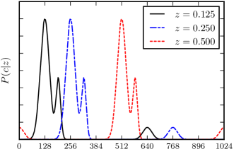
Figure 1: The probability distribution of observed colour $c$ for three different redshifts. The x-axis is the number of the colour bin, the galaxy may be put into. Here wee use $1024$ colour and redshift bins and the maximal redshift bin corresponds to $z=1$. Note that the shape of the distribution is assumed to be independent of $z$ and is only shifted towards higher colour values. This is a simplification with respect to real photometric redshift probabilities, where the shape of the PDF does depend on $z$. As we use a cyclic topology for this test-case, $z=1$ corresponds to $z=0$, and $c=0$ to $c=1024$, respectively. Therefore, the catastrophic outliers for $z=0.500$ (dotted red) reappear at the low colour values on the left.

The features we want to test for are asymmetric shape of $\mathbf{R}$ and the robustness to catastrophic outliers. As this is intended as a test-case, we make some simplifying assumptions about $P(c|z)$. First, we assume that the shape of $P(c|z)$ remains fixed when going to higher redshift and second we neglect the effect of the spectral type on the colour PDF. Catastrophic outliers are modelled by a small Gaussian PDF contribution which is offset from the main peak by half of the simulated interval length and whose height was chosen to be one tenth of the main peak. It should be stressed however, that once $\mathbf{R}$ is set up in a realistic way, no change is needed for the algorithm. In Fig. 1 we show the $P(c|z)$ we use and it should be explicitly said that this is not a real-world $P(c|z)$ but one that we designed to just look similar to a real-world $P(c|z)$ as in Benítez (2000).

3.3.2 Reconstruction of redshift space matter distribution from colour space data

For our reconstruction test we set up our simulation on an interval of length $L=1$ split into 1024 evenly sized pixels. As we are not interested in boundary effects here, we set the window function to unity for the whole interval.

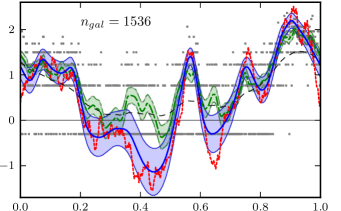
Figure 2: Reconstruction for a bias $b=1.5$ and $\bar{\rho}_{gal}=1000$ of a signal (red dotted curve) from data (grey dots) with Poissonian noise and typical spatial distortions as they occur in photometric redshift measurement. The data is where the point-wise inversion from (21) would place it and the thin evenly dashed black line shows the naive map $m_{na}$. The smooth blue line shows the classical reconstruction with the correct distortion matrix, the dash-dotted green line shows $m_{cl}^{u}$, a MAP map without the distortion of colour space taken into account. $1\sigma$ error levels are indicated by thin lines.

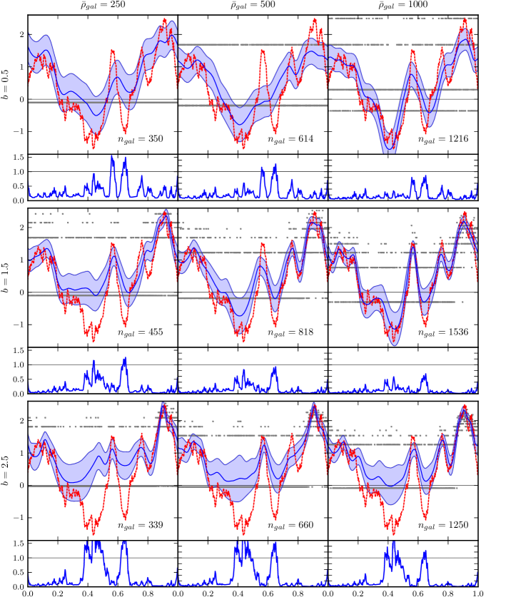
Figure 3: The top part of the nine panels show reconstructions of the same signal (dotted red) from data (grey dots) with Poissonian noise and typical spatial distortions as they occur in photometric redshift measurement. The data is where the point-wise inversion from (21) would place it. The blue line shows the classical signal reconstruction as proposed by our method with its $1\sigma$ error contours (thin blue lines). The bottom part of the nine panels show the characteristic residuals as defined by (28) for $500$ different data realisations for this signal.

In Figures 2 and 3 we show reconstructions of the signals with unit variance $\left\langle s_{x}^{2}\right\rangle_{(s)}=1$ from photometrically distorted data. In Fig. 3 we also show the characteristic residuals for this single signal $s_{t}$ when reconstructed by this technique, defined as

$$\operatorname{\mathrm{Res}}^{(s_{t})}=\left\langle(m_{d}-s_{t})^{2}\right\rangle_{(d|s_{t})}$$ (28)

where $m_{d}$ is the map as it is reconstructed from the data $d$. In practice, we do this average for 500 different data realisations of the same signal $s_{t}$. This shows in which regions the algorithm generally performs badly for a specific signal and where it does well independently from the data realisation. One may notice in Fig. 3, that in actual data realisations the galaxy numbers vary for different biasses while keeping $\bar{\rho}_{gal}$ constant. This has to be expected because the average galaxy density is only the same for different biasses, when averaged over all signal realisations. This may affect the comparability of the characteristic residuals for different biasses, but not for the same bias and different galaxy densities.

The first thing to notice about the reconstructions is that in all cases they are pretty smooth even though the noise in the data is considerable and also the original signal has far more power on small scales. This is against common knowledge that MAP maps pick up a lot of noise. What prevents this in our case is the distortion matrix which act as a smoothing operation on the observed data such that $m_{cl}$ itself becomes smooth again.

In Fig. 2 we also show a classical reconstruction $m_{cl}^{u}$ that does not take the distortion of data space into account, i.e. it assumes that $\mathbf{R}=\kappa^{\mathtt{t}}\mathbb{1}$. Compared to our full reconstruction $m_{cl}$ one can see that neglecting the colour space distortion results in severe difficulties to get even the shape right. Instead of voids $m_{cl}^{u}$ even sees peaks at $0.4$ and $0.65$. Although large peaks are detected, their height is slightly underestimated because some events are scattered away which $m_{cl}^{u}$ is not aware of. The full reconstruction on the other hand can even reshape the void region located at $0.4$, despite the abundance of events in that region originating from the large peak at $0.9$. Looking at the characteristic residuals in Fig. 3 reveals that this is true for most data realisations.

In Fig. 3 we show reconstructions of the same signal for different simulation parameters and their average residuals. In the reconstructions, one can make out two obvious trends for our simplified model:

• The higher the galaxy density, the better the overall reconstruction (note in particular the decreasing level of $\operatorname{\mathrm{Res}}^{(s_{t})}$).

• The higher the bias the better becomes the reconstruction of peaks, but the worse becomes the reconstruction of void regions.

Both observations are not surprising, since higher galaxy density means that the response is sampled with less Poissonian noise, so one expects the reconstruction to become better. Higher bias on the other hand sharpens the contrast such that peaks are selectively sampled with high accuracy whereas the galaxy density in void regions is reduced. This trend is also reflected by the error bars which tighten up in overdense regions for biasses larger than one, but not so for $b=0.5$.

The example for $b=0.5$ and $\bar{\rho}_{gal}=500$ shows that data variance can make a big difference. Although the number of galaxies is nearly twice as large as in the panel to its left, the peak at $0.55$ is hardly detected at all. Looking at the residuals reveals that this is simply an artefact of a lucky data realisation for the low density case and an unlucky one for the middle density case.

Looking at the characteristic residuals one notices, that for $b=0.5$ the general trend of the signal (i.e. the largest Fourier modes) can be detected even for very low galaxy densities, while sharp peaks and ditches are even difficult to resolve for $\bar{\rho}_{gal}=1000$. For $b=1.5$ and $b=2.5$ the overdense regions can be resolved even for low density of events, while the voids are difficult to reshape for low galaxy densities.

It should be mentioned however, that the poor resolution of voids is also a problem of this specific example, because every void region has an overdense region that scatters events into the void ($0.9$ into $0.4$ and $0.15$ into $0.65$). Had we chosen an example where two void regions scatter into each other, the resolution of these voids would be much better.

Table 1: As an indicator for the quality of different reconstructions this table lists $\left\langle\lVert m-s_{t}\rVert_{2}^{2}\right\rangle_{(s_{t})}$, the average $L_{2}$-distance from reconstruction $m$ to true signal $s_{t}$, where the $s$-average runs over 500 random signal configurations.

		$\bar{\rho}_{gal}=250$	$\bar{\rho}_{gal}=500$	$\bar{\rho}_{gal}=1000$
	$m_{na}$	1.03	1.03	0.78
$b=0.5$	$m_{cl}^{u}$	0.34	0.27	0.23
	$m_{cl}$	0.31	0.15	0.16
	$m_{na}$	0.68	0.63	0.58
$b=1.5$	$m_{cl}^{u}$	0.36	0.33	0.32
	$m_{cl}$	0.25	0.19	0.15
	$m_{na}$	0.74	0.70	0.68
$b=2.5$	$m_{cl}^{u}$	0.60	0.57	0.54
	$m_{cl}$	0.41	0.34	0.28

In Table 1 we list the average residuals of 500 reconstructions of different signals. The naive map $m_{na}$ is in all cases the worst reconstruction. Especially for low galaxy densities it is painfully close to the average residual of a zero map, which is expected to be unity for a Gaussian signal with unit variance. This tells above all one thing: for a reconstruction in the low signal to noise regime one must include some knowledge about the signal. For a low bias $m_{cl}^{u}$ and $m_{cl}$ have roughly the same error level when the galaxy density is low. When $\bar{\rho}_{gal}$ rises, both maps become better but what surprises is that $m_{cl}$ seems to saturate over $\bar{\rho}_{gal}\geq 500$ at an error level of $\approx 0.15$. Considering the fact, that the distortion of the signal inevitably destroys some information, the question arises, if this is already the optimum. Therefore, we let the same signals be processed without noise in the response, i.e. with perfect data and found for $b=0.5$ that without Poissonian noise $m_{cl}$ has an average residual of $0.09$ and $m_{na}$ of $0.27$. So we see that for the signals with $\bar{\rho}_{gal}=500$ and $\bar{\rho}_{gal}=1000$ there is still is some margin to be gained by even higher galaxy densities, but not much. It is remarkable, that $m_{na}$ with noiseless data comes not even close to the performance of $m_{cl}$ with medium galaxy density.

There is one anomaly worth noticing, namely the increase of the residuals from $b=1.5$ to $b=2.5$ observed for all maps but $m_{cl}^{u}$ in particular, which comes from catastrophic outliers scattering into void regions. Since count rates for $b=2.5$ are only large at big overdensities and remain small even for smaller peaks, $m_{cl}^{u}$ makes a small peak from scattered events in voids. The same holds also for $m_{na}$, but this map does not react as quickly on few events as $m_{cl}^{u}$ does, which explains the modest deterioration of $m_{na}$ and the striking difference for $m_{cl}^{u}$.

3.4 Signal inference from independent data sets

In real world surveys like SDSS there might be both available, accurate spectroscopic galaxy redshift and abundant less certain photometric redshift data. Can the former help to better localise the latter?

Our formalism allows to combine both data sets by defining

$$d=\left(d^{(1)},\,d^{(2)}\right)=\left(\mathbf{R}^{(1)},\,\mathbf{R}^{(2)}\right)^{\mathtt{t}}\kappa\,\mathrm{e}^{b\,s}$$ (29)

and business is as usual.

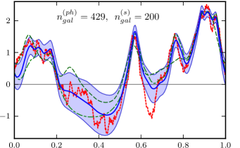
Figure 4: Classical reconstruction of a signal (red dotted line) from two independent data sets (data points not shown) for a bias of $b=1.5$, $\bar{\rho}^{\,ph}_{gal}=250$ and $\bar{\rho}^{s}_{gal}=60$. The reconstruction from photometric data alone is shown as a dark-green evenly dashed curve, the reconstruction from spectroscopic data as a green dash-dotted curve. The combined analysis of both data sets is shown as an blue smooth curve. The $1\sigma$ error level of the combined reconstruction is indicated by the thin blue solid line. For the other reconstructions it was omitted for clarity.

In principle this allows to combine any two data sets, but now consider the case where $d^{(1)}$ are data from photometric redshift measurement and $d^{(2)}$ from spectroscopic redshift measurement. As such, we model $\mathbf{R}^{(1)}$ as in section 3.3.1. Since spectroscopic redshift measurement is far more accurate than photometric redshift measurement, we assume spectroscopic redshift measurements to be exact, i.e. $\mathbf{R}^{(2)}=\mathbb{1}\kappa$ with $\kappa$ being the zero-response (12).

In Fig. 4 we show a reconstruction for one data realisation $d^{(1)}$ and $d^{(2)}$ with a bias $b=1.5$. The combined reconstruction $m_{cl}^{(s+ph)}$ mostly follows the reconstruction from spectroscopic data $m_{cl}^{(s)}$, especially in overdense regions such as from $0.8$ to $1.0$ and $0.5$ to $0.6$. This is an expected behaviour, since in this case $b=1.5$ and therefore overdense regions are accurately sampled even with the low average galaxy density $\bar{\rho}^{s}_{gal}=60$. And since the spectroscopic data have no spatial error, they dominate the reconstruction in this regime. However, in regions where spectroscopic galaxies are rare, the combined reconstruction sometimes deviates substantially from $m_{cl}^{(s)}$ (most conspicuous from $0.2$ to $0.4$). The crucial point to note is that the combined reconstruction is not an average of the two reconstructions $m_{cl}^{(s)}$ and $\smash{m_{cl}^{(ph)}}$ as can be seen at $0.4$ to $0.5$ and $0.6$ to $0.7$ where the combined reconstruction lies below the others. Therefore, the optimal combination of the two datasets is non-trivial and non-linear.

The statistics for 500 different signal realisations (not shown) confirm that the combination is more than just a superposition of the two single-dataset reconstructions.

3.5 X-ray astronomy via coded mask telescopes

Thanks to the generic structure of our approach, we can also apply it to a completely different problem. One such problem is the detection of extended sources in coded mask aperture systems.

Coded aperture systems were originally proposed by Dicke (1968) for the purpose of detecting point-like X-ray sources. In this scheme an absorbing plate with a pattern of pinholes is placed in front of a detector and the shadow of this plate on the detector allows with the knowledge of the plate pattern to unfold the count distribution and infer the positions of the X-ray sources. However, this technique becomes much more difficult, when the light sources are extended and not just point sources.

We now demonstrate that it is in principle possible to map out extended sources with our method, when count rate and bias are high enough. Adapting our method to this problem, the mixing matrix in this case must be the coded mask pattern that lets light pass for open pixels and shields it completely for dark pixels. Hence we only need the pattern of a coded mask for our distortion matrix. Today’s coded masks have an optimised pattern, but for our purpose the originally proposed random pattern (Dicke, 1968) of blocking and transparent pixels is sufficient.

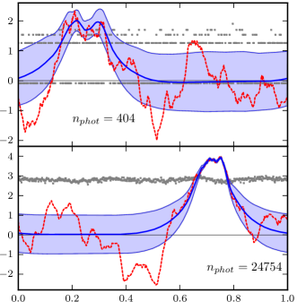
Figure 5: Reconstruction of a signal (red dotted line) from data (grey dots) that mimic the behaviour of coded mask apertures with a bias $b=2.5$ and an average photon count rate $\bar{n}_{phot}=500$. The $m_{cl}$ reconstruction (blue smooth curve) shows only the largest peak of the signal, and some of its substructure. $1\sigma$-error levels are indicated by thin lines. Being completely useless, the naïve map $m_{na}$ was omitted.

In Fig. 5 we show two reconstructions on an interval with 512 pixels from data obtained via a random pattern coded mask. In this set-up it is only possible to detect the largest peak, therefore we use a rather large bias of $b=2.5$. It is remarkable that a surprisingly low number of photons $n_{phot}=404$ is sufficient to detect the peak at position $0.25$ in the top panel and even some bits of its substructure. In regions where the algorithm can not see the signal, the error bar widens up to the interval +1 to -1. This is a good consistency check, because this is expected for a signal with unit variance when no information on the signal is available.

The lower panel in Fig. 5 shows a reconstruction from a signal with an extremely high peak. Although such high peaks and count rates are quite rare, it is interesting how much details of the peak can be reconstructed with extremely small error range. Note that the smaller peak at $0.15$ in this example – although comparable in size to the peak in the top panel – is not detected at all. This is due to the overwhelmingly larger brightness of the largest peak at $0.75$ whose photons hit the same detector, but with an approximately $\mathrm{e}^{b\cdot 4}/\mathrm{e}^{b\cdot 2}\approx 148$ higher rate. The Poissonian noise from the larger peak overlays with the photons from the smaller peak, rendering it impossible to detect.

This is however not yet a fully realistic set-up and further effort must be put into refining this technique, as sometimes false peaks (with narrow error bars) turn up in the reconstruction. It is possible that this problem has already been amended by the invention of especially designed coded masks which we did not consider here.

3.6 Reconstruction with $s$-dependent distortion

We now address the problem where the distortion matrix depends on the signal to be reconstructed. The paradigm for this is the measurement of distance via redshift. Due to the peculiar velocities of galaxies with respect to the Hubble frame the comoving distance of galaxies can not exactly be calculated from their redshift. Note that there needs not be a coordinate transformation from redshift into real space, because objects with different positions may have the same redshift. Therefore, the mapping from real to redshift space is not injective, thus not invertible.

In particular, the gravitational pull of matter overdensities affects the peculiar velocities of galaxies. So if one wants to unfold the large-scale matter distribution in the universe by measuring angular positions and redshifts of galaxies, one has to take the distorting effects of matter on the redshift space into account. What makes this problem so particularly demanding is that the distortion operator, which transforms the real-space matter distribution into the observed redshift space matter distribution, depends on the real-space matter distribution itself which is to be reconstructed.

One has to be aware that the assumption that the matter field is sampled by a Poissonian process will fail at some point when going to ever smaller scales. Here we show up problems one has to face even in an idealistic set-up where the forward transformation from real to redshift space is perfectly known.

3.6.1 A statistical model for redshift space distortions

We now address the forward problem of constructing the redshift space galaxy distribution from a known real space matter distribution and try to keep our model as simple as possible. In the following, “redshift space” will always refer to our model redshift space which we construct with the same characteristic features as the redshift space found in nature. To that we develop a simple model which bases on a few generic assumptions. We first distinguish between two regimes: the linear and the non-linear regime of large-scale structure formation.

The linear regime is dominated by the peculiar velocities from the bulk motion of matter in the direction of large-scale overdensities. The matter flow in this regime is described quantitatively by linear perturbation theory as

$$\vec{v}_{l}=\frac{2f(\Omega)}{3aH\Omega}\vec{\nabla}\Phi$$ (30)

where $f(\Omega)\equiv\frac{d\log D_{+}(a)}{d\log a}\approx\Omega^{0.6}$ and $D_{+}$ is the linear growth factor of matter perturbations during the matter dominated era of the universe. The potential $\Phi$ is determined by

$$\nabla^{2}\Phi=4\pi G\bar{\rho}a^{2}\biggl{(}\frac{\rho-\bar{\rho}}{\bar{\rho}}\biggr{)}$$ (31)

where $\bar{\rho}$ is the mean matter density and $G$ is the gravitational constant (Mukhanov, 2005, chapter 6). The first to point out the connection between linear perturbation theory of matter perturbations and redshift space distortions was Kaiser (1987), for an extensive review on the topic we refer to Hamilton (1998). The bottom line is that linear distortions lead to an amplification of overdensities and a depletion of underdensities in redshift space.

However, this relation can only be valid on large scales, because small scale inhomogeneities rather collapse and form a gravitationally bound object for which linear perturbation theory fails. Experimentally this manifests in the deviation of the redshift space matter power spectrum from the expected power spectrum of linear perturbation theory for wave numbers $k\ga 0.15\,h\,\mathrm{Mpc}^{-1}$ (e.g. Percival et al. (2007); Smith et al. (2003)). Therefore, when we calculate $v$ from (30), we first apply a tophat lowpass filter on the potential $\Phi$ and continue with (30). This way, only the largest modes of the linear velocity field are resolved which we use in our set-up of the distortion matrix $\mathbf{R}$.

The non-linear regime sets in when the perturbations in the matter distribution collapse and form gravitationally bound objects of numerous galaxies. In redshift space this presents itself as elongated structures along the line of sight which are called ‘fingers-of-god’. As the gravitational force of any galaxy on any other in the superstructure are relevant, this is effectively an N-body problem which is known to behave chaotically. So in contrast to the linear contribution to the redshift space distortions, the non-linear contribution to the peculiar velocity cannot be explicitly given. It is therefore in order, to resort to a statistical approach here, and we assume that objects in the non-linear regime are completely virialised and that their velocities have a Boltzmann PDF.

From the virial law of classical mechanics (Landau & Lifshitz, 1966) we can obtain a relation between the gravitational potential and the time averaged velocity: $\left\langle\vec{v}^{2}\right\rangle_{t}=-\left\langle\Phi\right\rangle_{t}$. Assuming $\left\langle\Phi\right\rangle_{t}\approx\Phi$ yields a relation between the potential and the velocity dispersion. We now assume that the velocity PDF for the objects in a virialised system is given by a Boltzmann factor

$$P(\vec{v}_{nl})\,d\vec{v}\propto\exp\biggl{(}-\frac{\vec{v_{nl}}^{2}}{\Phi}\biggr{)}d\vec{v}.$$ (32)

which guarantees the right velocity dispersion. That non-linear velocity distortions are given by a Maxwellian distribution is a common assumption used by many authors (e.g. Peacock & Dodds, 1994; Heavens & Taylor, 1995; Tadros et al., 1999; Tadros & Efstathiou, 1996). The other school of thought models the non-linear velocity distribution as an exponential pairwise PDF, i.e. $P(v)=\bigl{(}2^{1/2}\sigma\bigr{)}^{-1}\exp\bigl{(}-2^{1/2}|v|/\sigma\bigr{)}$ (e.g. Bromley et al., 1997; Hamilton, 1995; Ratcliffe et al., 1998).

We now have to blend the two regimes into one general expression. Therefore, we extend (32) and make the ansatz

$$P(v_{\|})\propto\exp\biggl{(}-\frac{(v_{\|}-v_{l,\|})^{2}}{2F(\Phi)}\biggr{)}$$ (33)

where $F$ is a continuous function to be determined and $v_{l,\|}$ is the component along the line of sight of the linear velocity field determined by (30). The function $F$ must have the following limiting behaviour in order to interpolate between the linear and non-linear regime:

$$\lim_{\Phi\rightarrow-\infty}F(\Phi) =|\Phi|/2 \lim_{\Phi\rightarrow+\infty}F(\Phi) =0.$$

Since $F$ stands in the denominator, it must never become exactly $0$, hence it must also not change sign. Apart from that, the Boltzmann factor should play little to no role in the linear regime where $\Phi$ is above a threshold $\Phi_{0}$ over which we do not assume objects to be virialised. In principle, we should therefore require that $F\approx 0$ in these regions, i.e. exact measurement. In practice on the other hand, every measurement comes with uncertainties and even in the linear regime galaxies can have unpredictable small peculiar velocities. Subsuming this as ‘measurement uncertainties’, it makes sense to require that $F(\Phi)\geq\sigma_{0}$ which includes this instrument noise naturally in our formalism. In other words, we turn the shortcoming of our method to model exact measurement into the feature to always include a minimal error with variance $\sigma_{0}$. For the non-linear regime we assume that galaxies are only virialised with their potential excess $\Delta\Phi=\Phi-\Phi_{0}$, i.e. $F(\Delta\Phi)=-\Delta\Phi/2$.

One possibility to smoothen the transition from linearly to non-linearly dominated regions is by a tilted hyperbola such as

$$F(\Delta\Phi)=\frac{1}{4}\biggl{(}\sqrt{\bigl{(}\Delta\Phi+2\sigma_{0}^{2}\bigr{)}^{2}+\tau^{2}}-\Delta\Phi\biggr{)}+\frac{1}{2}\sigma_{0}^{2},$$ (34)

which has the advantage of only introducing one more free parameter $\tau$ which controls the smoothness of the transition.

This allows to write the distortion matrix for the transformation from real to redshift space as

$$\mathbf{R}_{ij}\equiv P(z_{i}|x_{j},\,\rho)\propto\exp\biggl{(}-\frac{(z_{i}-v_{l\|,j})^{2}}{2F(\Phi_{j}-\Phi_{0})}\biggr{)}.$$ (35)

Altogether we now have five free parameters to control the behaviour of our self-built velocity dispersion model, namely

• the strength of the linear velocity distortions, which is given for a cosmological model

• the width of the tophat lowpass filter for the linear velocity field, which can be determined by analysing the redshift space matter power spectrum as $k\la 0.15\,h\,\mathrm{Mpc}^{-1}$ Percival et al. (2007); Smith et al. (2003)

• $\tau$ adjusting the smoothness of the transition from linear to non-linear behaviour

• $\Phi_{0}$ for the zero-level of the gravitational potential under which non-linear effects kick in

• and $\sigma_{0}$ for any further measurement error.

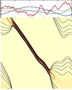
Figure 6: Example for a possible distortion matrix. Note that the maximum of the distribution is not necessarily on the diagonal due to the linear redshift distortions. The log-spaced contours indicate levels of equal height. On top the signal (solid red line) that generates this distortion matrix, the potential (blue dash-dotted line) and the streaming velocity resulting from linear theory (green dotted line) – all scaled to comparable amplitudes. Note that the strength of the linear displacement is slightly larger than in our simulation to make its effect better visible to the eye.

As we are aiming at a proof of concept, we also take the gravitational constant, which adjusts the strength of the non-linear effects, as a free parameter to generate visible effects with our distortion model. In Fig. 6 we show the mixing matrix as it was used in the reconstructions of the following section.

As before, we use the conjugate gradient method for minimization of the probability Hamiltonian. This method requires the derivative of the Hamiltonian and therefore also the derivative of $\mathbf{R}[s]$ with respect to $s$. However, for our model a direct calculation of the gradient of $\mathbf{R}$ is not feasible, as it would demand the evaluation of $N_{pix}^{3}$ difficult to compute entries of $\mathbf{R}$, which would pose strong limitations on the performance, as the evaluation of $\mathbf{R}$ already is the bottleneck of our algorithm. Therefore we make the approximation, that the contribution of $\frac{\delta\mathbf{R}}{\delta s}$ is small compared to the other terms in the gradient of $H$, i.e.

$$\begin{split}\frac{\delta H}{\delta s_{k}}&=\bigl{(}\mathbf{S}^{-1}s\bigr{)}_{k}-\biggl{(}\frac{d}{\mu}-1\biggr{)}^{\mathtt{t}}\frac{\delta\mu}{\delta s_{k}}\\ &\approx\sum_{j}\mathbf{S}^{-1}_{kj}s_{j}-\sum_{i}\biggl{(}\frac{d}{\mu}-1\biggr{)}_{i}\mathbf{R}_{ik}\,b\,\mathrm{e}^{b\,s_{k}}.\end{split}$$ (36)

Although this is an approximation, a simulated annealing process started from the resulting map never finds a better minimum than this. Therefore we can safely regard the minimum obtained with the approximated gradient as the true minimum of $H$.

Similarly, we are forced to make the same approximation when we approximate the error bars as already mentioned in 3.2.3.

3.6.2 Results from the reconstruction of the real space matter distribution from redshift space data

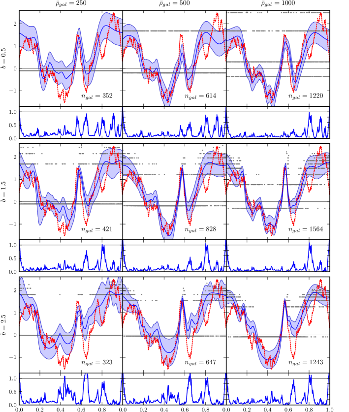
Figure 7: The top part of the nine panels show the real space reconstructions of the same signal (red dotted line) from data given in redshift space (grey dots) with Poissonian noise where the transformation from real to redshift space is given by (35). The data is where the point-wise inversion from (21) would place it. The smooth blue curve shows the classical signal reconstruction as proposed by our method with its $1\sigma$ error contours (thin blue lines). The bottom part of the nine panels show the characteristic residuals as defined by (28) for $500$ different data realisations of this signal.

We set up a run of 500 signal reconstructions on an interval of length $L=1$ with 1024 equally sized pixels. Due to our limited interval length we had to restrict ourselves to signals whose maximum peak was less than $3.5$, as for peaks higher than this value the tail of the smeared-out peaks overlap with the tail on the other side.

For each signal realisation $s$ we generate one possible data realisation $d$ and do three different types of reconstructions, namely the naive map $m_{na}$ from 3.2.1, a MAP reconstruction neglecting redshift space distortions $m_{cl}^{u}$ and the full MAP map including the model redshift space distortions $m_{cl}$. Fig. 7 shows our $m_{cl}$ reconstruction for one signal but for different $b$ and $\bar{\rho}_{gal}$ settings, along with the characteristic residuals $\operatorname{\mathrm{Res}}^{(s_{t})}$ for the reconstruction of the signal in the lower panels. For our model we find the following general trends

• the higher the galaxy density, the better the reconstruction

• the higher the bias, the worse the reconstruction of voids, but peaks on the other hand are better reconstructed

The reasons for these trends are the same as in section 3.3.2. The reconstructions from galaxies with redshift distortions is therefore similar in many respects to the one with photometric redshifts.

Note that the centre peak in the data (at $0.55$) shows a clear dislocation from its signal counterpart in direction of the massive at $0.9$ – an effect due to the linear velocity distortions. The $m_{cl}$ reconstruction however, being aware of the redshift distortions introduced by the large massive, places the peak at the right spot in all reconstructions. Interestingly, for large biasses this peak is well resolved even for very low galaxy densities as the characteristic residuals show.

Yet there are limitations for the reconstructions as can be seen in the indentations flanking the largest peak at positions $0.8$ and $1.0$. Although being comparable in size to the peak at $0.55$, they are not resolved in any reconstruction, and this even remains the case for extremely large $\bar{\rho}_{gal}$ which we do not show here. Apparently, these structures are irreversibly lost in the shadow that the larger peak at $0.9$ casts on close-by smaller structures. This is also not unexpected, as the distortion matrix $\mathbf{R}$ is set up in a way that large peaks become smeared out over large distances, whereas small peaks remain localised. Therefore, the smaller peak appears as an extension of the plateau. The most important characteristic of this kind of error is that it does not improve with higher $\bar{\rho}_{gal}$ in contrast to areas where more information can be gained by reducing the noise (e.g. wide void regions).

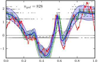
Figure 8: Reconstruction of the same signal (red dotted line) as in Fig. 7 for an average galaxy density $\bar{\rho}_{gal}=500$ and galaxy bias $b=1.5$. The data (grey dots) is where the point-wise inversion from (21) would place it and the thin evenly dashed black line shows the naïve map $m_{na}$. In addition to our redshift corrected map $m_{cl}$ (blue smooth curve) we also show a MAP reconstruction $m_{cl}^{u}$ neglecting redshift distortions (green dash-dotted curve). Note that $m_{cl}^{u}$ and $m_{na}$ pick up basically the same features, but $m_{cl}^{u}$ responds much quicker to an excess of galaxies. $1\sigma$ error levels are indicated by thin lines.

In Figure 8 we show the centre panel from Fig. 7 with the reconstruction for $b=1.5$ and $\bar{\rho}_{gal}=500$ again but also the naive map $m_{na}$ and the MAP map neglecting redshift space distortions $m_{cl}^{u}$. At first sight, one notices the poor guess that $m_{na}$ gives, which we take as an argument that Bayesian analysis is inevitable to tackle this problem.

The more interesting competitor for the MAP map including the correction of redshift space distortions $m_{cl}$ is $m_{cl}^{u}$. In general, the shape of the reconstruction is very similar which is as it should be, as both algorithms base on the same principles and work on the same data set. Yet there are some distinct features that make the difference. Most prominent is of course the correct treatment of linear redshift space distortions of $m_{cl}$ in contrast to $m_{cl}^{u}$ which sees the void from $0.15$ to $0.3$ further depleted and the peak at $0.55$ displaced towards the massive on the right. Another more subtle difference is that $m_{cl}^{u}$ picks up more small scale features from the data as can be seen in region $0.8$ to $1.1$. This is due to the smoothing effect of $\mathbf{R}^{\mathtt{t}}$ on the $m_{cl}$ reconstruction as already discussed in section 3.3.2.

In contrast to the photometric case from section 3.3.2, the error bars do not tighten up in overdense regions. However this has to be expected, since our model was set up in a way, that the position uncertainty in the neighbourhood of large peaks is largest. In particular, this makes the detection of substructure in large peaks nearly impossible.

Table 2: As an indicator for the quality of different reconstructions this table lists $\left\langle\lVert m-s_{t}\rVert_{2}^{2}\right\rangle_{(s_{t})}$, the average $L_{2}$-distance from reconstruction $m$ to true signal $s_{t}$, where the $s$-average runs over 500 random signal realisations.

		$\bar{\rho}_{gal}=250$	$\bar{\rho}_{gal}=500$	$\bar{\rho}_{gal}=1000$
	$m_{na}$	0.88	0.81	0.71
$b=0.5$	$m_{cl}^{u}$	0.29	0.24	0.21
	$m_{cl}$	0.26	0.20	0.15
	$m_{na}$	0.71	0.62	0.54
$b=1.5$	$m_{cl}^{u}$	0.27	0.23	0.21
	$m_{cl}$	0.23	0.18	0.14
	$m_{na}$	0.75	0.70	0.66
$b=2.5$	$m_{cl}^{u}$	0.48	0.42	0.38
	$m_{cl}$	0.41	0.34	0.28

For a signal-independent view on the reconstruction quality we list in Table 2 the average $L_{2}$-distance from reconstruction to true signal for 500 different signal reconstructions.

The reconstruction benefit from including redshift space distortions seems not to be overwhelming but tends to be larger if bias and galaxy density rise. Notably for $m_{cl}^{u}$ the effects from linear and non-linear redshift distortions partially cancel each other for the parameters chosen here and thereby improve the performance of $m_{cl}^{u}$. This is because non-linear redshift space distortions smear out large peaks while linear redshift distortions compress large overdensities. If we turn off linear redshift distortions and set up $\mathbf{R}$ only with our virialisation model for non-linear redshift distortions, we get the interesting effect that the average $L_{2}$-distance of $m_{cl}$ to $s_{t}$ becomes smaller, but for $m_{cl}^{u}$ it increases instead.

So far we have assumed that the underlying redshift distortion model is perfectly known and its parameters are the same both for data generation and reconstruction phase. In a set-up for measured data this is not the case. Neither is there a perfect model for the forward transformation from real to redshift space, nor are its parameters accurately measured. How severely parameter errors affect the reconstruction has not been scrutinised, but can be aim of further investigation. Still, if this model was adapted and applied to measured data, the above mentioned reconstruction characteristics and limitations would hold.

3.6.3 Refining the distortion model

In section 3.6.1 we have introduced a model for the transformation from real to redshift space in a statistical way. One important step was to apply a lowpass filter to the potential before the linear velocity field was calculated. However, similarly to using only the low modes of the perturbation for calculating the velocity distortions, it would be reasonable to use only the high modes for calculating the velocity dispersion.

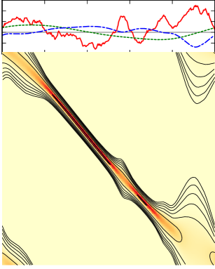
Figure 9: Example for a possible distortion matrix where the potential leading to the non-linear redshift distortions is high-pass filtered. Note that the maximum of the distribution is not necessarily on the diagonal due to the linear redshift distortions. The log-spaced contours indicate levels of equal height. On top the signal (solid red line) that generates this distortion matrix, the potential (blue dash-dotted line) and the streaming velocity resulting from linear theory (green dotted line) – all scaled to comparable amplitudes. Note that in contrast to Fig. 6 the sharp peak at $0.55$ is now a separate collapsed object with its own velocity dispersion.

This is because the non-linear velocity dispersion predominantly depend on small-scale physics. If a halo with many galaxies collapses, the energy that the galaxies gain from the collapse is only the difference from their former potential energy and the potential energy after they have entered the collapsed structure. The velocity dispersion is hence not proportional to the full potential, but only to the fraction of the potential that the galaxies have actually fallen. Assuming that the galaxies in the collapsed structure are all from the vicinity of the collapsed object, this fraction can be estimated as the high frequency component of the potential. In the picture of energy conservation one may look upon this as

• the low frequency part of the potential adds to the energy of linear velocity distortions and

• the high frequency part of the potential adds to the non-linear velocity component.

In Fig. 9 we show the resulting distortion matrix of the modified model for the same signal as in Fig. 6.

When we set up the velocity distortions this way, we find that the problem becomes severely harder and the MAP solution ultimately fails to give reasonable results. Interestingly it is the low bias case $b=0.5$ which is hardest. This is most likely due to the fact that the response for $b=0.5$ makes a double peak from large peaks, i.e. bifurcates the peak. This misleads the MAP map to make two peaks out of one, which can lead to very weird behaviour. This bifurcation will eventually also happen for the larger biasses, if we turn up the strength of the velocity dispersion.

Our tests show, that the MAP solution via conjugate gradient minimization has severe problems with this bifurcation. We also employed a simulated annealing technique for minimization which gave us the same results. So we can say with good confidence, that in the case of a bifurcated response the MAP method may give the most likely map, but still a very bad reconstruction. With the complexity of the distortion matrix at this point we finally have reached a limit for the MAP method.

3.6.4 Comparison to Metropolis-Hastings sampling

The question now arises, whether the MAP method is already the optimal reconstruction given the data or not. According to theory, this should not be the case, because the MAP map minimizes $\left\langle\lVert m-s_{t}\rVert_{0}\right\rangle_{(s|d)}$, but the $L_{0}$-norm is a rather distorted measure of distance. Unfortunately, the posterior is too complex that $\left\langle s\right\rangle_{(s|d)}$ can be calculated directly. However, if there was a way to approximate the posterior by another PDF, that is easier to evaluate, we may be able to calculate $\left\langle s\right\rangle_{(s|d)}$ directly. Since our interest is not in the detailed shape of the posterior, but our aim is simply to evaluate integrals over the posterior quickly, we may approximate the posterior $P(s|d)$ by

$$\widetilde{P}(s)\equiv\frac{1}{N}\sum_{i=1}^{N}\delta(s-s_{i})$$ (37)

where we construct the $s_{i}$ using a Metropolis-Hastings MCMC method. In principle the chain can start from any map $s_{0}$, but for the sake of skipping the burn-in phase, we start our MCMC from $m_{cl}$. At any given point $s_{n}$ we generate a small variation $\delta s$ with the same power spectrum as the signal, but with far smaller amplitude and set $s_{n+1}=s_{n}+\delta s$. We accept or reject this new sample according to the Metropolis-Hastings criterion (Binder, 1997, e.g. ). This gives us a chain of maps where consecutive samples are correlated, but after some steps the correlation vanishes.

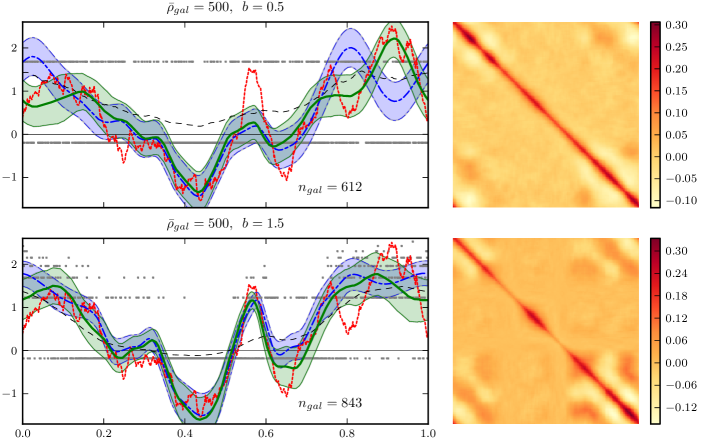
Figure 10: On the left two reconstructions for different settings of the biasses $b=0.5$ and $b=1.5$. The signal appears as a red dotted line, the data (grey dots) are where the naïve data inversion from (21) would place it. The naïve map (thin evenly dashed line) is the smoothed data and shows signs of bifurcation at $0.9$. The $m_{cl}$ reconstruction (blue dash-dotted curve) interprets the bifurcation as two different peaks, while the posterior mean (smooth green curve) does not. $1\sigma$ error contours are indicated by thin lines. The pictures on the right show the uncertainty covariance matrix of the Metropolis-Hastings reconstruction. Note the long-range influence of the structure at $0.9$.

Since a MCMC is expensive with respect to computation time, we can not run several hundred reconstructions but have to be satisfied with the evaluation of selected cases. Therefore, we show in Fig. 10 only three reconstructions without the characteristic residuals as we did before. As one can see there, the sampling method and the MAP method give very similar results in the region from $0.2$ to $0.7$ where the redshift space distortions are comparatively small, although the posterior mean tends to be a bit better especially in the $b=1.5$ case. Similarly, the width of the error bars is virtually the same in this region.

But not so in the region from $0.7$ to $1.2$. There, the MAP approach is taken in by the bifurcation and gives a very bad guess from $0.7$ to $1.1$ where it places peaks instead of valleys and a valley instead of a peak. And what makes the situation problematic indeed is that the estimated error bars are rather small there. The algorithm therefore completely misjudges its accuracy. As already mentioned above, the situation improves a bit for the bias $1.5$ but the problem is still there.

The sampling method on the other hand does the right thing in the interval $0.7$ to $1.1$. It nicely reshapes the largest peak and at the place of the side-peak $0.75$ which is in the ‘shadow’ of the larger peak at $0.9$ it widens the error bar to remain on the safe side. If this is just by chance of unlucky data cannot be judged for sure at this point. For the larger bias $1.5$ the improvement is not quite so good because the shadow on nearby structures is much stronger.

The impression that the reconstruction quality of the average map from Metropolis-Hastings sampling is much better than the $m_{cl}$ reconstruction also manifests itself in the $L_{2}$-distance which we list in Table 3.

Table 3: $L_{2}$-distance of reconstruction to signal for three reconstructions two of which are shown in Fig. 10. Note that there is hardly any improvement of the classical map from $\bar{\rho}_{gal}=500$ to $\bar{\rho}_{gal}=1000$ for $b=0.5$ while the posterior average improves by about 40%. For the larger bias $b=1.5$ the difference between $m_{cl}$ and posterior average becomes less palpably.

	$\bar{\rho}_{gal}=500$	$\bar{\rho}_{gal}=1000$	$\bar{\rho}_{gal}=500$
	$b=0.5$	$b=0.5$	$b=1.5$
$\lVert m_{cl}-s_{t}\rVert_{2}^{2}$	0.42	0.41	0.24
$\lVert\left\langle s\right\rangle_{(s|d)}-s_{t}\rVert_{2}^{2}$	0.17	0.10	0.16

Note also how the uncertainty covariance matrix in Fig. 10 changes from $b=0.5$ to $b=1.5$. To understand what lies beneath one has to look at the Gaussian approximation of the posterior $P(s|d)\approx\mathcal{N}\exp\bigl{(}j^{\mathtt{t}}s-s^{\mathtt{t}}\mathbf{D}^{-1}s/2\bigr{)}$. Here $\mathcal{N}=\mathrm{e}^{-j^{\mathtt{t}}\mathbf{D}j/2}/|2\pi\mathbf{D}|$ is a normalisation factor and $j$ summarises all terms of the probability Hamiltonian of first order in $s$. Direct calculation yields

$$\left\langle s\right\rangle_{(s|d)}\approx\mathcal{N}\int\!\mathcal{D}s\,s\,\mathrm{e}^{j^{\mathtt{t}}s-s^{\mathtt{t}}\mathbf{D}^{-1}s/2}=\mathbf{D}j.$$ (38)

Enßlin et al. (2009) call $j$ the information source because it excites the posterior mean from a zero-map to a non-zero state. One can show that in our problem $j$ contains a term linear in $d$ and additional terms. Therefore, equation (38) tells how the posterior mean reacts on additional data. Hence the pictures of the propagator in Fig. 10 show how the posterior map is constructed from the information source $j$ and introduces a correlation length in the map.

In void regions the correlation length is longer than in overdense regions because the Poissonian noise is larger there. If there were no other source of uncertainty but the Poissonian noise, the band would be tightest in the most overdense regions. But there is an additional source of uncertainty, namely the velocity dispersion from the redshift distortion model. Therefore, in overdense regions the correlation length of the propagator does not collapse, but shows a pattern of strong correlation and anticorrelation, as can be seen in the region from $0.7$ to $1.2$ in both cases. Comparing the correlation length to the distortion matrix in Fig. 9 shows that this is in good agreement to the correlation induced from the distortion matrix. The main difference in the correlation matrix of the example with $b=1.5$ is that the contrast is sharper and that the diagonal is much more structured.

4 Conclusions

Many reconstruction problems in cosmology suffer not only from large noise but also from substantial measurement uncertainties. While it is possible that some measurement uncertainties will be ameliorated in the future by more sophisticated techniques, other sources of uncertainty are fundamental such as cosmic variance and galaxy redshift distributions. Areas where this applies are real space LSS reconstructions from galaxy counts in redshift space, but also consistent treatment of photometric redshift. For precision cosmology with galaxies it is therefore of paramount importance to incorporate these uncertainties in the analysis.

Here we have presented a novel method how spatially distorted log-normal fields as they occur in density field reconstruction can be reconstructed in a Bayesian way. This method was developed in the framework of information field theory which we outlined in section 2. We showed that the IFT moment calculation ultimately foots on the minimization of the expected $L_{2}$-weighted error of the reconstruction. Where exact moment calculation from the posterior was not possible, we argued how the correct map – the posterior mean – could be approximated by a MAP approach.

We developed a data model for a log-normal signal with Poissonian noise where the response can be non-local. We even allowed for the case, in which the distortion of data space could depend on the signal that was to be reconstructed. The resulting problem is so complex that it could only be solved approximately via numerical minimization of its probability Hamiltonian.

For a test of our approach we performed simulations where we constructed mock signals, produced mock data thereof and tried to reconstruct the underlying signal by numerical minimization of the probability Hamiltonian.

We tested our reconstruction code on three different distortion problems which were

• data with typical distortions as they appear in photometric redshift measurement,

• coded mask aperture problems as they appear in X- and $\gamma$-ray astronomy and

• real space matter reconstruction from redshift distorted data.

For the latter we developed a model for the forward problem to construct redshift space data from real space galaxy distributions and where the distortion was dependent on the underlying matter distribution that was to be measured. We were able to tackle this problem with a MAP approach. However, after further complication of the distortion operator we found that the MAP method does not live up to its expectations. Instead, we could show that approximating the posterior via Metropolis-Hastings sampling could give much more accurate reconstructions. Therefore we think, that for such complicated problems the MAP method gives misleading results and should be superseded by more powerful however also computationally more demanding approaches such as sampling the posterior PDF.

For the coded mask data we were able to identify the largest peaks and showed that it is even possible to reconstruct their substructure if the count rates are high enough. An application of this approach to real X- or $\gamma$-ray data should be possible but before doing so, some effort must be spent to make the approach robuster to false detection of peaks.

At last, the reconstruction of a redshift space signal from photometric redshift data proved to be very fruitful. In many cases we were able to reconstruct the underlying matter distribution remarkably well. Since the colour space distortion is independent of the underlying signal, an application of our approach to large data sets is feasible.

We also showed that in the IFT framework it is possible to easily combine data sets with different error characteristics. We considered the problem of combining photometric redshift data with large uncertainties and spectroscopic data that are very accurate in position. Our analysis showed that even with a low abundance of accurate data it is possible to improve the reconstruction from distorted data with large abundance as long as there is room for improvement.

In all cases we found that Bayesian analysis of the problem is inevitable for the noise level we were considering. We also showed that the reconstruction becomes significantly worse when the data were distorted, but the data space distortion was neglected during the reconstruction. Therefore we think that including the data space distortions in future precision analysis is inevitable.

Since the assumptions of our method are based on a few generic principles we are confident that further areas will be found where our work will be appreciated.

Appendix A Notation

Having to deal extensively with field variables, one needs a shorthand notation for the calculus. Hence we define a vector space whose elements are fields – in this sense we use the terms ‘vector’ and ‘field’ interchangeably. The dot product in this vector space is defined by

$$v^{\mathtt{t}}w\equiv\int dx\,v(x)w(x).$$ (39)

Instead of writing the field variable in round brackets we usually use a notation where the variable is in subscript to make the correspondence to finite dimensional vector spaces more obvious.

We also use tensors of higher rank over this vector space, most notably matrices. Analogously to (39), we define

$$\bigl{(}\mathbf{M}v\bigr{)}(x) =\int dy\,M(x,\,y)v(y)$$

$$\bigl{(}\mathbf{M}\mathbf{N}\bigr{)}(x,y) =\int dz\,M(x,\,z)N(z,\,y)$$

and so on.

We also need a field space equivalent of the frequently used rules

$$\frac{\partial}{\partial x_{i}}x_{j} =\delta_{ij} \frac{\partial}{\partial x_{i}}\sum_{j}x_{j}k_{j} =k_{i}.$$

For all practical applications this is enough as one deals only with a finite number of pixels, however all equations remain valid if one defines the functional derivative according to Peskin & Schroeder (1995, chap. 9) as

$$\frac{\delta}{\delta J_{x}}J_{y} =\delta(x-y) \frac{\delta}{\delta J_{x}}\int dy\,J_{y}\Phi_{y} =\Phi_{x}.$$

This blends in naturally with our definition of the vector product (39).

Vectors are printed in normal font with indices omitted. Matrices are in bold font where possible, with the notable exception of derivatives of vectors such as $\frac{\delta\mu}{\delta s}$. To avoid an ambiguity in the sequence of the indices we define for derivations that the new index shall be last, i.e.

$$\left(\frac{\delta\mu}{\delta s}\right)_{ij}\equiv\frac{\delta\mu_{i}}{\delta s_{j}}.$$

All functions are understood to act component-wise, that is $f(v)$ should be read as $f(v)_{i}\equiv f(v_{i})$. In particular, this also applies to fundamental operations, such as multiplication and division: $(v\cdot w)_{i}\equiv v_{i}\,w_{i}$ and $(v/w)\equiv v_{i}/w_{i}$. Note also that we do not adopt Einstein’s summation convention, such that an expression as $v_{i}\,\mathrm{e}^{w_{i}}$ should in fact be read as the number $v_{i}$ multiplied by the number $\mathrm{e}^{w_{i}}$.

In this notation subtle differences do matter, but it shortens the formulas considerably. Here some intricate examples:

$$s^{\mathtt{t}}\mathbf{S}s=\sum_{i,j}\mathbf{S}_{ij}\,s_{i}\,s_{j}=\mathbf{S}_{ij}\,s^{i}\,s^{j}$$

$$\bigl{(}v(\mathbf{S}w)\bigr{)}_{i}=v_{i}\,\Bigl{(}\sum_{j}\mathbf{S}_{ij}w_{j}\Bigr{)}=v_{i}\,\mathbf{S}_{ij}w^{j}$$

$$(v\,w^{\mathtt{t}})_{ij}=v_{i}w_{j}$$

$$(v\mathbf{S})_{ij}=v_{i}\mathbf{S}_{ij}$$

$$(v^{\mathtt{t}}\mathbf{S})_{i}=\sum_{j}v_{j}\mathbf{S}_{ji}=v^{j}\mathbf{S}_{ji}$$

Appendix B Generating mock signals with Gaussian covariance matrix

The aim is to generate signals with Gaussian covariance matrix

$$\left\langle ss^{\mathtt{t}}\right\rangle_{(s)}=\mathbf{S}.$$ (40)

By this definition, $\mathbf{S}$ is symmetric and positive definite such that it has a root, i.e. there exists a matrix $\mathbf{T}$ such that $\mathbf{S}=\mathbf{T}^{\mathtt{t}}\mathbf{T}$. We now show that the mock signal can be generated by convolving a vector of Gaussian random numbers $r$ with $\mathbf{T}$: $s=\mathbf{T}r$

Without loss of generality we restrict our reasoning to the case where the Gaussian random numbers in $r$ have unit variance, such that the prior for $r$ is

$$P(r)=\prod_{j}\frac{1}{\sqrt{2\pi}}\mathrm{e}^{-r_{j}^{2}/2}=\frac{\mathrm{e}^{-r^{2}/2}}{|2\pi\mathbb{1}|^{1/2}}.$$ (41)

Here the product runs over all pixel indices. From $r$ we construct the signal vector $s$ by application of $\mathbf{T}$, which can be understood as a smoothing procedure for the random values. Note also that only in this step different points of the signal become correlated with each other – the entries of $r$ are by virtue of the random nature of its entries uncorrelated.

We now have to prove that this procedure gives the desired prior for $s$:

$$P(s) =\int\!\mathcal{D}r\,\delta(s-\mathbf{T}r)\cdot P(r)$$

$$=\int\!\mathcal{D}q\int\!\mathcal{D}r\,\frac{1}{|2\pi\mathbb{1}|}\mathrm{e}^{-iq^{\mathtt{t}}(s-\mathbf{T}r)}\,\frac{\mathrm{e}^{-r^{2}/2}}{|2\pi\mathbb{1}|^{1/2}}$$

$$=\frac{1}{|2\pi\mathbb{1}|}\int\!\mathcal{D}q\,\mathrm{e}^{-q^{\mathtt{t}}\mathbf{S}q/2-\imath q^{\mathtt{t}}s}$$

$$=\frac{1}{|2\pi\mathbf{S}|^{1/2}}\,\mathrm{e}^{-s^{\mathtt{t}}\mathbf{S}^{-1}s/2}=\mathcal{G}(s,\,\mathbf{S})$$

As source for random numbers we use the ‘Mersenne Twister’ random number generator which offers a pseudo random number sequence with a period of $2^{19937}-1$ (Matsumoto & Nishimura, 1998). Its advantages are speed and very good randomness. In particular, we use its implementation from the GNU Scientific Library (gsl).

Note that this procedure gives an easy and robust way to test whether the constructed signal has indeed the desired covariance

$$s^{\mathtt{t}}\mathbf{S}^{-1}s=r^{\mathtt{t}}\mathbf{T}^{\mathtt{t}}\mathbf{S}^{-1}\mathbf{T}r=r^{\mathtt{t}}r\approx N_{pix}$$

where we have used that $r$ is a vector of $N_{pix}$ Gaussian random numbers of unit variance in the last step. In other words, for a Gaussian random field $s$ the number $s^{\mathtt{t}}\mathbf{S}^{-1}s$ should roughly give the dimension of $s$.

References

- Benítez (2000) Benítez N., 2000, ApJ, 536, 571
- Bertschinger et al. (1990) Bertschinger E., Dekel A., Faber S. M., Dressler A., Burstein D., 1990, ApJ, 364, 370
- Bialek et al. (1996) Bialek W., Callan C. G., Strong S. P., 1996, Physical Review Letters, 77, 4693
- Binder (1997) Binder K., 1997, Reports on Progress in Physics, 60, 487
- Branchini et al. (1996) Branchini E., Plionis M., Sciama D. W., 1996, ApJ, 461, L17
- Bromley et al. (1997) Bromley B. C., Warren M. S., Zurek W. H., 1997, ApJ, 475, 414
- Cole et al. (2000) Cole S., Lacey C. G., Baugh C. M., Frenk C. S., 2000, MNRAS, 319, 168
- Coles & Jones (1991) Coles P., Jones B., 1991, MNRAS, 248, 1
- Cornwell & Evans (1985) Cornwell T. J., Evans K. F., 1985, A&A, 143, 77
- Dicke (1968) Dicke R. H., 1968, ApJ, 153, L101
- Duane et al. (1987) Duane S., Kennedy A. D., Pendleton B. J., Roweth D., 1987, Physics Letters B, 195, 216
- Efstathiou (2000) Efstathiou G., 2000, MNRAS, 317, 697
- Enßlin et al. (2009) Enßlin T. A., Frommert M., Kitaura F. S., 2009, Phys. Rev. D, 80, 105005
- Enßlin & Frommert (2010) Enßlin T., Frommert M., 2010, ArXiv e-prints
- Erdoğdu et al. (2006) Erdoğdu P., Lahav O., Huchra J., et al. 2006, MNRAS, 373, 45
- Erdoğdu et al. (2004) Erdoğdu P., et al., 2004, MNRAS, 352, 939
- Frieden & Wells (1978) Frieden R. R., Wells D. C., 1978, Journal of the Optical Society of America (1917-1983), 68, 93
- Fry & Gaztanaga (1993) Fry J. N., Gaztanaga E., 1993, ApJ, 413, 447
- Geman & Geman (1984) Geman S., Geman D., 1984, IEEE Trans. Pattern Anal. Mach. Intell., 6, 721
- Goldberg (2001) Goldberg D. M., 2001, ApJ, 550, 87
- Green (1990) Green P. J., 1990, IEEE Trans. Med. Imag, pp 84–93
- Gull & Daniell (1978) Gull S. F., Daniell G. J., 1978, Nature, 272, 686
- Hamilton (1995) Hamilton A. J. S., 1995, in S. Maurogordato, C. Balkowski, C. Tao, & J. Tran Thanh van ed., Clustering in the Universe Redshift distortions and in IRAS Surveys. p. 143
- Hamilton (1998) Hamilton A. J. S., 1998, in D. Hamilton ed., The Evolving Universe Vol. 231 of Astrophysics and Space Science Library, Linear Redshift Distortions: a Review. p. 185
- Hastings (1970) Hastings W. K., 1970, Biometrika, 57, 97
- Heavens & Taylor (1995) Heavens A. F., Taylor A. N., 1995, MNRAS, 275, 483
- Hebert & Leahy (1992) Hebert T. J., Leahy R., 1992, IEEE Transactions on Signal Processing, 40, 2290
- Hoffman & Zaroubi (2000) Hoffman Y., Zaroubi S., 2000, ApJ, 535, L5
- Hubble (1934) Hubble E., 1934, ApJ, 79, 8
- Huchra et al. (2005) Huchra J., Jarrett T., Skrutskie M., Cutri R., Schneider S., Macri L., Steining R., Mader J., Martimbeau N., George T., 2005, in Fairall A. P., Woudt P. A., eds, ASP Conf. Ser. 329: Nearby Large-Scale Structures and the Zone of Avoidance The 2MASS Redshift Survey and Low Galactic Latitude Large-Scale Structure. p. 135
- Jasche & Kitaura (2009) Jasche J., Kitaura F. S., 2009, ArXiv e-prints
- Jasche et al. (2009) Jasche J., Kitaura F. S., Li C., Enßlin T. A., 2009, ArXiv e-prints
- Jaynes (1957) Jaynes E. T., 1957, Phys. Rev., 106, 620
- Jenkins et al. (2001) Jenkins A., Frenk C. S., White S. D. M., Colberg J. M., Cole S., Evrard A. E., Couchman H. M. P., Yoshida N., 2001, MNRAS, 321, 372
- Jeong & Komatsu (2009) Jeong D., Komatsu E., 2009, ApJ, 703, 1230
- Kaiser (1987) Kaiser N., 1987, MNRAS, 227, 1
- Kauffmann et al. (1993) Kauffmann G., White S. D. M., Guiderdoni B., 1993, MNRAS, 264, 201
- Kayo et al. (2001) Kayo I., Taruya A., Suto Y., 2001, ApJ, 561, 22
- Kitaura et al. (2010) Kitaura F., Jasche J., Metcalf R. B., 2010, MNRAS, 403, 589
- Kitaura et al. (2009) Kitaura F. S., Jasche J., Li C., Enßlin T. A., Metcalf R. B., Wandelt B. D., Lemson G., White S. D. M., 2009, MNRAS, 400, 183
- Landau & Lifshitz (1966) Landau L. D., Lifshitz E. M., 1966, Mechanik
- Layzer (1956) Layzer D., 1956, AJ, 61, 383
- Lemm (1999) Lemm J. C., 1999, ArXiv Physics e-prints
- Lemm (2001) Lemm J. C., 2001, in A. Mohammad-Djafari ed., Bayesian Inference and Maximum Entropy Methods in Science and Engineering Vol. 568 of American Institute of Physics Conference Series, Bayesian field theory and approximate symmetries. pp 425–436
- Lemm et al. (2001) Lemm J. C., Uhlig J., Weiguny A., 2001, European Physical Journal B, 20, 349
- Lemm et al. (2005) Lemm J. C., Uhlig J., Weiguny A., 2005, European Physical Journal B, 46, 41
- Martínez & Saar (2002) Martínez V. J., Saar E., 2002, Statistics of the Galaxy Distribution. Chapman &
- Matsubara (2008a) Matsubara T., 2008a, Phys. Rev. D, 78, 109901
- Matsubara (2008b) Matsubara T., 2008b, Phys. Rev. D, 78, 083519
- Matsumoto & Nishimura (1998) Matsumoto M., Nishimura T., 1998, ACM Trans. Model. Comput. Simul., 8, 3
- Metropolis et al. (1953) Metropolis N., Rosenbluth A. W., Rosenbluth M. N., Teller A. H., Teller E., 1953, J. Chem. Phys., 21, 1087
- Mukhanov (2005) Mukhanov V., 2005, Physical Foundations of Cosmology
- Navarro et al. (1996) Navarro J. F., Frenk C. S., White S. D. M., 1996, ApJ, 462, 563
- Neyrinck et al. (2009) Neyrinck M. C., Szapudi I., Szalay A. S., 2009, ApJ, 698, L90
- Nityananda & Narayan (1982) Nityananda R., Narayan R., 1982, Journal of Astrophysics and Astronomy, 3, 419
- Nunez & Llacer (1990) Nunez J., Llacer J., 1990, Ap&SS, 171, 341
- Nusser & Haehnelt (1999) Nusser A., Haehnelt M., 1999, MNRAS, 303, 179
- Oh & Frieden (2009) Oh C., Frieden R. B., 2009, Optics Communications, 282, 2489
- Peacock & Dodds (1994) Peacock J. A., Dodds S. J., 1994, MNRAS, 267, 1020
- Peebles (1980) Peebles P. J. E., 1980, The large-scale structure of the universe
- Percival (2005) Percival W. J., 2005, MNRAS, 356, 1168
- Percival et al. (2007) Percival W. J., Nichol R. C., Eisenstein D. J., Frieman J. A., Fukugita M., Loveday J., Pope A. C., Schneider D. P., Szalay A. S., Tegmark M., Vogeley M. S., Weinberg D. H., Zehavi I., Bahcall N. A., Brinkmann J., Connolly A. J., Meiksin A., 2007, ApJ, 657, 645
- Peskin & Schroeder (1995) Peskin M. E., Schroeder D. V., 1995, An Introduction to Quantum Field Theory. Westview Press
- Ratcliffe et al. (1998) Ratcliffe A., Shanks T., Parker Q. A., Fong R., 1998, MNRAS, 296, 191
- Schmoldt et al. (1999) Schmoldt I. M., Saar V., Saha P., Branchini E., Efstathiou G. P., Frenk C. S., Keeble O., Maddox S., McMahon R., Oliver S., Rowan-Robinson M., Saunders W., Sutherland W. J., Tadros H., White S. D. M., 1999, ApJ, 118, 1146
- Shaya et al. (1995) Shaya E. J., Peebles P. J. E., Tully R. B., 1995, ApJ, 454, 15
- Shewchuk (1994) Shewchuk J. R., 1994, An Introduction to the Conjugate Gradient Method Without the Agonizing Pain. published in the web
- Smith et al. (2003) Smith R. E., Peacock J. A., Jenkins A., White S. D. M., Frenk C. S., Pearce F. R., Thomas P. A., Efstathiou G., Couchman H. M. P., 2003, MNRAS, 341, 1311
- Springel et al. (2005) Springel V., White S. D. M., Jenkins A., Frenk C. S., Yoshida N., Gao L., Navarro J., Thacker R., Croton D., Helly J., Peacock J. A., Cole S., Thomas P., Couchman H., Evrard A., Colberg J., Pearce F., 2005, Nature, 435, 629
- Tadros et al. (1999) Tadros H., Ballinger W. E., Taylor A. N., Heavens A. F., Efstathiou G., Saunders W., Frenk C. S., Keeble O., McMahon R., Maddox S. J., Oliver S., Rowan-Robinson M., Sutherland W. J., White S. D. M., 1999, MNRAS, 305, 527
- Tadros & Efstathiou (1996) Tadros H., Efstathiou G., 1996, MNRAS, 282, 1381
- Vogeley et al. (2004) Vogeley M. S., Hoyle F., Rojas R. R., Goldberg D. M., 2004, in Diaferio A., ed., IAU Colloq. 195: Outskirts of Galaxy Clusters: Intense Life in the Suburbs Mapping the cosmic web with the Sloan Digital Sky Survey. pp 5–11
- Wang et al. (2008) Wang G., Fu L., Qi J., 2008, Physics in Medicine and Biology, 53, 593
- Webster et al. (1997) Webster M., Lahav O., Fisher K., 1997, MNRAS, 287, 425
- White & Frenk (1991) White S. D. M., Frenk C. S., 1991, ApJ, 379, 52
- Wittman (2009) Wittman D., 2009, ApJ, 700, L174
- Yahil et al. (1991) Yahil A., Strauss M. A., Davis M., Huchra J. P., 1991, ApJ, 372, 380