Search for Outbursts in the Narrow 511-keV Line from Compact Sources Based on INTEGRAL Data

{}^{\,*}

and E.M.Churazov^1,2

¹ Max Planck Institut für Astrophysik, Karl-Schwarzschild-Str. 1, Postfach 1317, D-85741 Garching, Germany
² Space Research Institute, Russian Academy of Sciences, Profsoyuznaya ul. 84/32, Moscow 117997, Russia

Received September 14, 2009

We present the results of a systematic search for outbursts in the narrow positron annihilation line on various time scales ( $5\times 10^{4}$ – $10^{6}$ s) based on the SPI/INTEGRAL data obtained from 2003 to 2008. We show that no outbursts were detected with a statistical significance higher than $\sim$ $6\sigma$ for any of the time scales considered over the entire period of observations. We also show that, given the large number of independent trials, all of the observed spikes could be associated with purely statistical flux fluctuations and, in part, with a small systematic prediction error of the telescope’s instrumental background. Based on the exposure achieved in $\sim$ 6 yr of INTEGRAL operation, we provide conservative upper limits on the rate of outbursts with a given duration and flux in different parts of the sky.

Key words: interstellar medium, Galaxy, gamma-ray lines.

^∗ E-mail: tsygankov@iki.rssi.ru

INTRODUCTION

The positron annihilation line has been studied in detail by many authors based on data from various experiments since it was first discovered at the Galactic center (Johnson et al. 1972). Several positron generation models that completely or partly describe the observed line flux have been proposed to explain the nature of the observed emission: the synthesis of radioactive elements with the $\beta^{+}$ decay channel among daughter nuclei ( ${}^{22}Na$ , ${}^{26}Al$ , ${}^{44}Ti$ , ${}^{56}Ni$ , ${}^{57}Ni$ ) through supernova explosions, gamma-ray bursts, and hypernovae; the production of electron-positron pairs near pulsars and black holes; the interaction of cosmic rays with interstellar matter and the annihilation of dark matter particles (for a review, see, e.g., Teegarden and Watanabe 2006; Bandyopadhyay et al. 2009). In all of the positron generation mechanisms considered, the initial kinetic energy of the positrons is comparable to or appreciably higher than the electron rest mass.

If compact stellar objects are assumed to be the sources of positrons (see, e.g., Prantzos 2004; Weidenspointner et al. 2008), then the observed annihilation radiation need not be constant and can come in the form of outbursts. The slowing-down and annihilation time scale for positrons with a typical MeV energy is determined mainly by the density of the medium ( $n$ ): $\displaystyle\tau\sim 10^{5}\left(\frac{n}{10^{7}{\rm cm^{-3}}}\right)^{-1}$ s (Forman et al. 1986). Near compact sources (e.g., in accretion disks or on a stellar surface), the density can be very high and the actual constraint on the lifetime of a positron (including its slowdown and annihilation) can be related to the positron time of flight, of the order of seconds or shorter.

Possible flux variability at the Galactic center near 0.5 MeV was pointed out by a number of authors (see, e.g., Riegler et al. 1981). However, it was subsequently shown that the 511-keV line flux measured by a specific instrument clearly depended on the size of the instrument’s field of view; the larger the telescope’s field of view, the higher the flux it recorded (see, e.g., Teegarden 1994). In this way, a substantial fraction of the reports on flux variability in the annihilation line were disproved. It was also concluded from the detected dependence that the source of the annihilation radiation at the Galactic center is diffuse in nature.

In addition to the Galactic center, evidence for possible outbursts near 0.5 MeV has been found for compact sources: 1E 1740.7-2942 (Bouchet et al. 1991; Sunyaev et al. 1991) and Nova Musca (Sunyaev et al. 1992; Goldwurm et al. 1992, Gilfanov et al. 1994). The recorded broad emission lines in their spectra were considerably shifted relative to 511 keV to lower energies and were observed on a time scale of $\sim$ 0.5-2 days.

There are also a number of papers in which it is argued that the positron annihilation line flux from the Galactic-center region is constant (for a review, see., e.g., Purcell et al. 1997). The results of a search for transient events in the data of the first year of INTEGRAL operation are presented in Teegarden and Watanabe (2006) and also reveal no significant variability. Below, we present the results of a systematic search for outbursts in a narrow energy band, 508-514 keV, near the electron-positron annihilation line (about 99% of the flux in the annihilation line recorded from the Galactic center and a negligible flux from the continuum of sources with a hard energy spectrum fall within this band) based on six-year-long all-sky SPI/INTEGRAL observations. Our analysis was performed on outburst time scales from $5\times 10^{4}$ to $10^{6}$ s.

OBSERVATIONS

Our work is based on data from the SPI spectrometer (Vedrenne et al. 2003) onboard the INTEGRAL observatory (Winkler et al. 2003). This is one of the main INTEGRAL instruments and operates in the energy range 20–8000 keV. Owing to its high energy resolution ( $\sim$ 2 keV at energy 511 keV), it is ideally suited to investigating the properties of the positron annihilation line in the Galaxy. The spectrometer consists of 19 individual cooled germanium detectors (17 detectors remained operational after July 2004).

The main goal of this paper is a “blind” search (when the position of the sought-for object is not known in advance) for variable emission sources in the positron annihilation line. With such a formulation of the problem, the simplest and most reliable outburst detection method is to search for features on the count rate curve of the telescope. In this approach, the telescope’s optical scheme is roughly equivalent to a collimator with a field of view $\sim$ 30^∘ in diameter. Using a coded aperture and image reconstruction gives a gain in sensitivity only if the position of the outburst source is known in advance.

The INTEGRAL observatory has a high-apogee orbit with a revolution period around the Earth of about 3 days. The orbital parameters were chosen in such a way that the satellite is located outside the Earth’s radiation belts for $\sim$ 90% of the time, which allows continuous observations to be performed by the INTEGRAL instruments for a long time. The individual observations are the pointings of the INTEGRAL axis toward specific regions of the sky and have a typical duration of $\sim$ 2000 s. We used all of the available INTEGRAL data from February 2003 to October 2008 (the total exposure time was $\sim$ $7\times 10^{7}$ s).

Outburst Search Algorithms

For our analysis, we divided the entire celestial sphere into pixels 4 $\times$ 4 deg. in size, which roughly corresponds to the SPI angular resolution. A light curve consisting of the fluxes in an individual pointing in the 508-514 keV energy band was constructed in each of these pixels. Since the SPI field of view is much larger than the size of a single map pixel, each INTEGRAL pointing makes a contribution immediately to several tens of pixels on the map. Accordingly, the effective area of the spectrometer for each of these map pixels will be not the same but distributed in accordance with the shape of the SPI response at the energy under consideration (Sturner et al. 2003). The photon flux for each pointing in a specific map pixel was defined as the count rate averaged over all active detectors in the 508-514 keV energy band divided by the effective area of the spectrometer at energy $\sim$ 508 keV assigned to this map pixel in this pointing.

Refer to caption — Fig. 1: Exposure map of the SPI observations used here. The heavy solid lines indicate the three regions for which the results of our analysis are presented (a – the Galactic center (the distance from the center is R $<$ 25^∘), b – the Galactic plane (-120^∘ $<l<$ 120^∘, -25^∘ $<b<$ 25^∘), c – the entire sky); the contours represent the levels of equal exposure 0.07, 0.2, 0.7, 2, and 6 Ms.

Since the distribution of the effective area over the SPI field of view is highly nonuniform, the presence of persistent annihilation emission sources in the sky must lead to significant variations in the measured flux with source position in the SPI field of view. To eliminate these effects related to the presence of a persistent bright emission source in the 511-keV line at the Galactic center, its contribution was subtracted by assuming a bivariate Gaussian intensity distribution of this source with the center at the Galactic center and with a full width at half maximum (FWHM) along and across the Galactic plane of 9^∘and 6^∘, respectively (the parameters were taken from Churazov et al. (2010)).

Thus, the flux in units of phot cm^-2 s^-1 for a given pointing $i$ in a map pixel with coordinates $(x,y)$ was calculated as

F_{i}(x,y)=\frac{I_{det,i}(x,y)-I_{bkg,i}(x,y)-\int GC_{mod}(\alpha,\delta)\times A_{eff}(\alpha,\delta,x,y)\mathrm{d}\alpha\mathrm{d}\delta}{A_{eff}(x,y)},

(1)

where $I_{det,i}(x,y)$ and $I_{bkg,i}(x,y)$ are the detected and background (see below) count rates averaged over all active detectors for pointing $i$ in map pixel $(x,y)$ , respectively; $A_{eff}(\alpha,\delta,x,y)$ is the mean response of the SPI detectors in map pixel $(x,y)$ to a source of unit intensity with celestial coordinates $(\alpha,\delta)$ . For a more accurate determination of the contribution from the persistent source at the Galactic center, the integral in Eq. (1) was taken on a 0^∘.5 $\times$ 0^∘.5 grid.

In each map pixel, the entire observing time was divided into intervals of duration $\tau$ (from $5\times 10^{4}$ to $10^{6}$ s). Next, the flux within each interval $j$ was averaged as $<F_{(x,y),j}>=\frac{\Sigma(F_{(x,y),i}/\sigma_{(x,y),i}^{2})}{\Sigma(1/\sigma_{(x,y),i}^{2})}$ , where $<F_{(x,y),j}>$ is the weighted mean flux in interval $j$ , $F_{(x,y),i}$ and $\sigma_{(x,y),i}$ are the flux and the statistical flux error in the 508-514 keV channel in pointing $i$ in map pixel $(x,y)$ , respectively. Subsequently, we analyzed the deviation of this quantity from the mean flux $<F_{(x,y)}>$ over the entire light curve in a given map pixel obtained in a similar way. The significance of the flux deviation from the mean was calculated as $\frac{<F_{(x,y),j}>-<F_{(x,y)}>}{\sigma_{<F_{(x,y),j}>}}$ . We searched for outbursts in the 511 keV line on four time scales: 50, 100, 500, and 1000 ks.

As a result of the algorithm described above, we obtained the maps for each averaging time scale in each pixel of which the highest significance of a positive spike in flux relative to the mean in this map pixel was reflected.

Data Selection

Before their use, the data were cleaned from the observations performed during or immediately after powerful solar flares, detector calibration periods, and other events unrelated to the sought-for astrophysical effects.

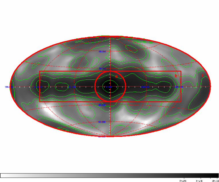
Due to peculiarities of the program of INTEGRAL observations, in our analysis we divided the entire celestial sphere into three parts (the Galactic center, the Galactic plane, and the entire sky) differing greatly in typical exposure time. These regions and the total exposure map are shown in Fig. 1. The exposure time in each map pixel was defined as the total exposure time $T_{i}$ in a given observation $i$ corrected for the ratio of the instrument’s effective area $A_{eff}(x,y)_{i}$ calculated for the telescope’s orientation in observation $i$ and coordinates on the celestial sphere corresponding to pixel $(x,y)$ to the maximum efficiency over the field of view at energy $\sim$ 508 keV ( $max(A_{eff})$ ). Thus, the formula used to calculate the exposure time in each map pixel appears as

$T(x,y)=\frac{\sum^{N}_{i=1}T_{i}\times A_{eff}(x,y)_{i}}{max(A_{eff})}$ ,

where $i$ is the pointing number, $N$ is the number of INTEGRAL pointings covering map pixel $(x,y)$ , $T_{i}$ is the total exposure time of observation $i$ , $max(A_{eff})$ is the maximum effective area of the spectrometer over the field of view at energy $\sim$ 508 keV, $A_{eff}(x,y)_{i}$ is the effective area of the spectrometer in map pixel $(x,y)$ for pointing $i$ .

We see that most of the observing time is allocated for the Galactic-center and Galactic-plane observations. In particular, the source 1E 1740.7-2942 whose spectrum previously exhibited a broad feature at energies 400-500 keV (Bouchet et al. 1991; Sunyaev et al. 1991) is located in this region.

Background Modeling

The recorded flux in the 511-keV line is strongly dominated by a variable (in time) background that is mainly related to the flux of charged cosmic-ray particles and their interaction with the SPI detectors and INTEGRAL constructions. We used two different methods to model the background flux at each instant of time:

(1) based on the use of the detector count rate above an upper energy threshold of 8 MeV (saturated events rate) as an indicator of the particle count rate (see, e.g.,Knodlseder et al. 2005; Churazov et al. 2005);

(2) based on the correlation of the fluxes in the 508-514 and 520-600 keV energy bands.

Both methods yield similar results, but here we used the background construction method (2) as a more appropriate one for the problem under consideration (see below). Since the SPI spectrometer has a good energy resolution, the 520-600 keV channel contains no contribution from the narrow 511-keV line and the ortho-positron continuum. The background count rate in the 520-600 keV energy band exceeds the count rate in the 508-514 keV band by a factor of 5, which allows no additional contribution to the statistical error of our results to be made. A serious advantage of the background model construction based on the count rate in a channel close in energy to the 508-514 keV one is an effective subtraction of the systematic features that manifest themselves in both bands.

Figure 2 shows the correlation of the count rates in the 508-514 and 520-600 keV energy bands. The abrupt changes in the correlation of the count rates correspond to the successive failure of two SPI detectors in December 2003 and July 2004. Because of the long-period background variations, we selected 14 epochs – the time intervals for which the correlation coefficients between the count rates in the investigated and reference energy channels were calculated independently.

It should be mentioned that the flux variations in the 520-600 keV band related to real astrophysical sources can cause flux variability in the 508-514 keV band. By definition, the background subtraction procedure is calibrated in such a way that if the ratio of the fluxes in the 508-514 and 520-600 keV bands is the same as that in the telescope’s instrumental background ( $R_{background}=F_{508-514}/F_{520-600}\sim 0.2$ ), then the expected flux in the 508-514 keV band after the background subtraction is zero. For typical astrophysical sources, the flux ratio is appreciably smaller. For example, for the spectrum of the Crab Nebula, $R_{Crab}=F_{508-514}/F_{520-600}\sim 0.09$ . Thus, a slight increase in flux in the 508-514 keV band will be more than compensated for by an increase in flux in the 520-600 keV. The measured flux in the 508-514 keV band corrected for the background will be $F_{508-514,Crab}-R_{background}\times F_{520-600,Crab}\sim-1.4\times 10^{-4}$ phot cm^-2 s^-1. Thus, negative spikes can appear on the light curve in the 508-514 keV band, provided that the continuum intensity of the source is very high. In this paper, we restrict our analysis to searching for only the positive spikes in the narrow 511-keV line.

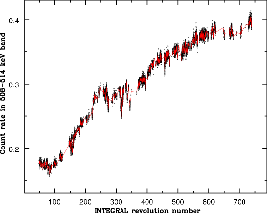
The quality of the prediction of the background radiation made by the method described above is illustrated by Fig. 3. The points in this figure indicate the measured count rate in the 508-514 keV energy band averaged over all active detectors on the scale of one INTEGRAL revolution; the solid line indicates the predicted background.

The Systematic Error

In addition to the statistical errors, there exist a number of sources of systematic errors when working with the SPI data. Thus, for example, the shape of the spectrum and the normalization of the background radiation cannot be predicted absolutely accurately. Nonideal subtraction of persistent emission sources in the 508-514 keV energy band can be yet another source of systematic errors.

The total error can be estimated from the distribution of flux significances over the entire map after the subtraction of the background flux and the constant flux in the 511-keV line from the source at the Galactic center (see Eq. (1)). If the systematic errors are small compared to the typical statistical errors in a given series of measurements and if there are no strong outbursts in the 511-keV line, then this must be a Gaussian distribution with a mean of 0 and a variance of 1.

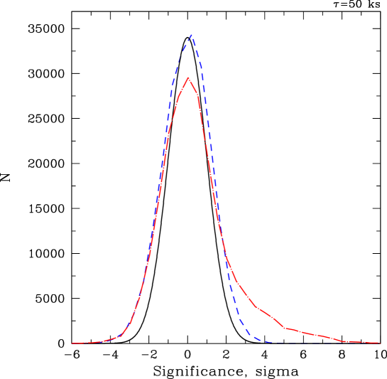
An example of such a distribution for the averaging time scale $\tau=50$ ks is shown in Fig. 4 (dashed line). For comparison, the solid line indicates a Gaussian distribution that is slightly narrower (see below) than the experimental one. To illustrate the quality of the subtraction of the central source in the 511-keV line, the dash-dotted line in Fig. 4 indicates the initial distribution of flux significances. The total error estimated by this method is valid only by assuming the absence of any real flux spikes in the annihilation line in the sky.

For the time scale under consideration, the total error in units of the standard deviation related to purely statistical fluctuations is $\sigma_{total}\simeq 1.25$ , which corresponds to a systematic error $\sigma_{sys}\simeq 0.75$ ( $\sigma^{2}_{total}=\sigma^{2}_{stat}+\sigma^{2}_{sys}$ ). The contribution from the systematic error increases with averaging time and reaches $\sigma_{sys}\simeq 0.90$ at $\tau=1000$ ks. These systematic errors also include the effects related to the possible presence of a persistent annihilation emission source different from the source at the Galactic center.

Thus, given the systematic component of the error, the actual significance of the detected outbursts is lower by 25-35%, depending on the averaging time scale, but here we disregarded this error component.

RESULTS

The effective area of the SPI spectrometer changes over a wide range, depending on the source position in its field of view. Accordingly, the same observation will have greatly differing statistical errors in different map pixels. Since our algorithm for analyzing the light curves selects the most significant positive flux deviations from the mean, statistical fluctuations can lead us to the selection of a value with a high error, while a slightly less significant point with a much smaller statistical error will be rejected. To determine more stringent upper limits on the flux variability in the 511-keV line, we rejected all points with errors above a certain value.

Thus, for example, to detect outbursts with a flux of $1\times 10^{-3}$ phot cm^-2 s^-1 with a 5 $\sigma$ significance, the statistical error should not exceed $2\times 10^{-4}$ phot cm^-2 s^-1. For each time scale, we used two limiting errors (Table 1).

Table 1: Limiting statistical errors of the experimental data points used in our analysis for four different averaging time scales.

Time scale,	Minimum	Limiting	Limiting
ks	error,	error 1,	error 2,
	10^-5 phot cm^-2 s^-1	10^-4 phot cm^-2 s^-1	10^-3 phot cm^-2 s^-1
50	8	2	2
100	8	2	2
500	4	1	1
1000	3	1	1

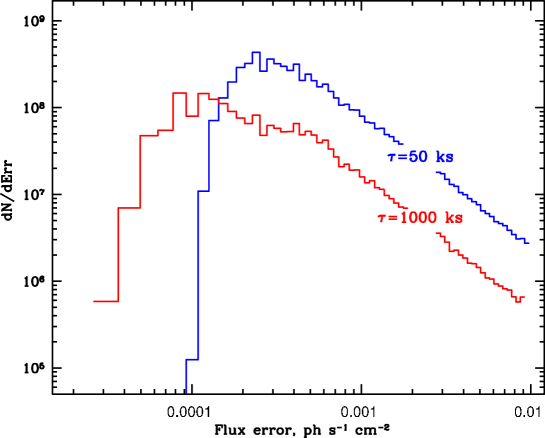
Figure 5 shows the distribution of statistical errors in each of the time bins (for two averaging time scales) over the entire sky map. The minimum statistical flux measurement error for a time bin of 50 ks is $\sigma_{min}\sim 8\times 10^{-5}$ phot cm^-2 s^-1. This means that we can detect an outburst with duration $t$ and flux $5\times\sigma_{min}\times(5\times 10^{4}/t)^{0.5}$ phot cm^-2 s^-1 with a significance of 5 $\sigma$ . The minimum error depends on the averaging time scale and decreases to $3\times 10^{-5}$ phot cm^-2 s^-1 for 1000-ks bins. However, as we see from Fig. 5, most of the flux measurements have a considerably larger statistical error, which reduces the effective sensitivity of our analysis.

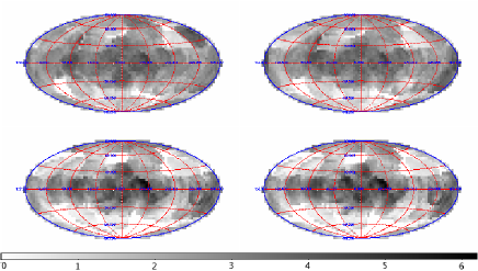
As a result, we constructed the maps of the highest significances of positive flux deviations in the 508-514 keV energy band from the mean in each map pixel. Figure 6a presents our results for all averaging time scales using the second set of limiting errors (see Table 1). We see that the positions of the most significant spikes in flux in the 511-keV line coincide with the region around the Galactic center and regions with a long observing time.

The increase in significance in these regions can be related to two effects: a large number of independent measurements (see below) and a possible contribution from nonideal subtraction of the diffuse source at the Galactic center.

To estimate the effect of an increase in the significance of the flux spike in the 511-keV line in the sky regions where the number of independent flux measurements is great, Fig. 7 shows the distribution of the probabilities to detect a maximum spike with a significance exceeding a given one by chance for three different numbers of independent trials. For high significance levels, this probability is, obviously, equivalent to the probability to detect such a spike for a Gaussian distribution multiplied by the number of independent trials.

The number of independent time bins in our analysis depends on the averaging time scale, the area of the analyzed sky region, and the maximum error in this averaging. The total number of INTEGRAL pointings used here is about 35 000. The number of independent points decreases as the averaged light curves are constructed.

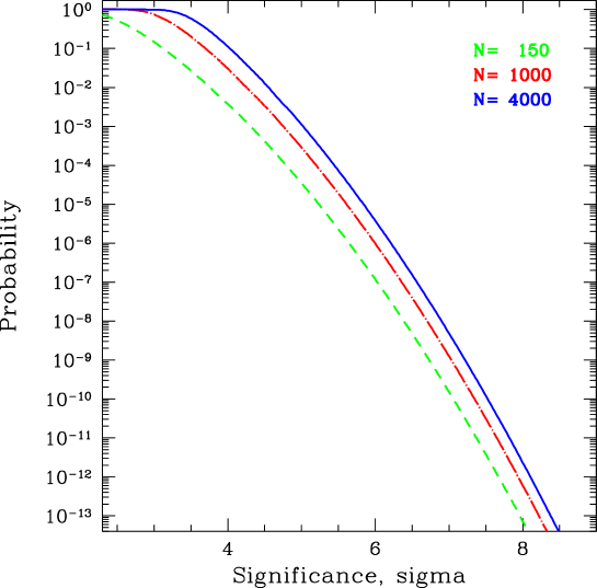
For example, the maximum recorded significance in the entire sky is $\sim$ $4.6\sigma$ for 100-ks time bins with errors of less than $2\times 10^{-4}$ phot cm^-2 s^-1. If the number of independent bins there is $\sim$ 2500, then the probability to find a spike with such a significance by chance is $P\sim 5\times 10^{-3}$ . Although the probability to detect such a spike only through statistical fluctuations is low, given the remaining inaccuracies in modeling the background (fractions of the statistical error), we use the corresponding value of $P\sim 5\times 10^{-3}$ phot cm^-2 s^-1 (Table 2) as a conservative upper limit on the maximum flux in an outburst of annihilation radiation.

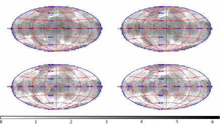
For clarity, Fig. 6b shows maps of the maximum significances of spikes similar to those shown in Fig. 6a but obtained by the Monte Carlo method: instead of the actually measured count rates in the 508-514 keV energy band, we substituted quantities with a Gaussian distribution with a mean of 0 and a variance equal to the error in a given measurement into the algorithm of our analysis. We see that purely statistical fluctuations (without any systematic effects) can lead to expected spikes comparable to the observed ones. For example, the Monte Carlo method shows that the expected maximum flux deviation from the mean for an averaging time scale of 100 ks and the second set of limiting errors (Table 1) at the Galactic center is $3\times 10^{-3}$ phot cm^-2 s^-1 with a significance of $\sim$ $3.5\sigma$ . In the actual data, these values are $1\times 10^{-3}$ phot cm^-2 s^-1 and 4.2 $\sigma$ , respectively.

Using the total observing time of a particular sky region, we can obtain upper limits on the rate of outbursts with a given duration and flux. Such estimates were made for a confidence level of $10^{-3}$ by assuming three different scenarios for the distribution of outbursts in the sky (see Fig. 1):

(i) uniform near the Galactic center (the distance from the center is R $<$ 25^∘);

(ii) uniform in the Galactic plane (-120^∘ $<l<$ 120^∘, -25^∘ $<b<$ 25^∘);

(iii) uniform over the entire sky.

The final results of our analysis are contained in Table 2: the maximum recorded significance ( $S_{max}$ , in units of the standard deviation) of an outburst in a given region and the corresponding flux deviation from the mean ( $F_{max}$ , in units of phot cm^-2 s^-1) are given for each of the sky regions under consideration (see above). All of the results are presented for four averaging time scales and two levels of limiting errors (Table 1). The value of $\nu$ limits the rate of outbursts with a flux $F>F_{max}$ in a given sky region at a confidence level of $10^{-3}$ (in units of yr^-1). The calculations were performed by assuming an equal probability of outbursts at any location of the region under consideration.

DISCUSSION

The maximum significance of the flux variability in the 511-keV line is observed near the Galactic plane at a Galactic latitude of $-30^{\circ}$ . This is the most interesting feature on the map, since the low-mass black-hole binary GRO J1655-40 can be a potential source of this outburst. The observed outburst in the 508-514 keV energy band coincides in time with an intense outburst in the standard X-ray energy band (Markwardt and Swank 2005) detected by many observatories in 2005.

Unfortunately, the duration of the source’s observations is too short to analyze this event in detail. The observed flux excess above the mean recorded by SPI in the 508-514 keV energy band is $\sim$ $4\times 10^{-4}$ and $\sim$ $2\times 10^{-3}$ phot cm^-2 s^-1 for the first and second sets of limiting errors, respectively. However, the absolute significance of this result (Table 2) is too low to talk about a reliable detection of the outburst.

It is important to note that the upper limits given in Table 2 refer only to the narrow emission line. If compact objects are the sources of the emission in the annihilation line, then its width can be much larger than several keV; it can also be shifted as a whole. In our case, the line flux will not be entirely in the 508-514 keV energy band and the algorithm we use will not show its significant variations. In Fig. 8, the fraction of the flux in the line centered at 511 keV falling within the 508-514 keV energy band is plotted against the FWHM of this line. Thus, a flux in the 508-514 keV energy band of only $\sim$ $2\times 10^{-4}$ phot cm^-2 s^-1 corresponds to a line flux of $\sim$ $6\times 10^{-3}$ phot cm^-2 s^-1 from Nova Musca at a 58-keV width of the line centered at 476 keV (Sunyaev et al. 1992; Gilfanov et al. 1991). Such an insignificant change in flux cannot be recorded with a significance of more than $\sim$ $2\sigma$ at an outburst duration of 100 ks even if the minimum statistical error is achieved for the time scale in question (Table 1).

Our upper limit on the flux variability in the narrow 511-keV line from 1E 1740.7-2942 is $\sim$ $5\times 10^{-4}$ phot cm^-2 s^-1 for an averaging time scale of 100 ks and the first set of limiting errors. Bouchet et al. (2009) present the results of a detailed spectral analysis of the emission from this microquasar based on three-year-long SPI and IBIS observations. The authors found neither a persistent, nor transient (on a time scale of 0.5–1 day), nor broad, nor narrow emission line near 511 keV in the source’s spectrum. They provide upper limits on the line detection on a time scale of one day, $\sim$ $7\times 10^{-4}$ phot cm^-2 s^-1.

CONCLUSIONS

We presented the results of a systematic search for outbursts in the narrow positron annihilation line on various time scales ( $5\times 10^{4}$ – $10^{6}$ s) based on the SPI/INTEGRAL data obtained from 2003 to 2008.

We showed that the background radiation level could be predicted on the basis of a reference energy band. Here, the 520-600 keV energy band containing no contribution from the narrow 511-keV line and the ortho-positron continuum was used for this purpose. A serious advantage of the background model construction based on a reference energy channel is an effective subtraction of the systematic features that manifest themselves in both bands.

We showed that no outbursts were observed with a statistical significance higher than $\sim$ $6\sigma$ for any of the time scales considered in the entire sky. The maximum annihilation flux amplitude depends on the maximum errors and time scale used (Table 2). We estimated the effect of statistical fluctuations on the detection of outbursts of annihilation radiation. Thus, for example, using the Monte Carlo method, we showed that a maximum flux deviation from the mean of $3\times 10^{-3}$ phot cm^-2 s^-1 was reached at the Galactic center with a significance of $\sim$ $3.5\sigma$ for an averaging time scale of 100 ks and statistical errors no larger than $2\times 10^{-3}$ phot cm^-2 s^-1. In contrast, the experimental value of the most significant positive flux deviation from the mean in this region is $1\times 10^{-3}$ phot cm^-2 s^-1 with a significance of $\sim$ $4.2\sigma$ .

The statistical flux measurements errors in the 508-514 keV energy band allow an outburst of duration $t$ and flux $5\times\sigma_{min}\times(5\times 10^{4}/t)^{0.5}$ phot cm^-2 s^-1 (where $\sigma_{min}\sim 8\times 10^{-5}$ phot cm^-2 s^-1) to be detected with a significance of 5 $\sigma$ .

Based on the exposure achieved in $\sim$ 6 yr of INTEGRAL operation, we provide conservative upper limits on the rate of outbursts with a given duration and flux in different parts of the sky (for a confidence level of $10^{-3}$ ). Thus, for example, one might expect no more than $\sim$ 3 outbursts per year in the entire sky.

Based on the recorded variability, we provide constraints on the flux in the narrow annihilation emission line in the spectrum of the transient GRO J1655-40 during its outburst in 2005. The most conservative upper limit does not exceed $\sim$ $2\times 10^{-3}$ phot cm^-2 s^-1.

ACKNOWLEDGMENTS

We wish to thank R.A. Sunyaev for the discussion of our results and helpful remarks. This work was supported by grant no. NSh-5579.2008.2 from the President of Russia, the “Origin, Structure, and Evolution of Objects in the Universe” Program of the Presidium of the Russian Academy of Sciences, and the Russian Foundation for Basic Research (project no. 07-02-01051). We used data from the INTEGRAL Science Data Center (Versoix, Switzerland) and the Russian INTEGRAL Science Data Center (Moscow, Russia).

Table 2: Results of our analysis. For each of the averaging time scales under consideration, we give the maximum recorded significance of an outburst in a specific sky region (

S_{max}

, in units of the standard deviation) and the corresponding flux deviation from the mean (

F_{max}

, in units of phot cm^-2 s^-1). The second column provides the rate of outbursts in a given sky region (

\nu

, in units of yr^-1).

Sky region	Rate of	Averaging time scale, ks
	outbursts, $\nu$	50		100		500		1000
	$\nu$	$S_{max}$	$F_{max}$	$S_{max}$	$F_{max}$	$S_{max}$	$F_{max}$	$S_{max}$	$F_{max}$
Limiting errors 1
Galactic center	10.1	3.9	$6.9\times 10^{-4}$	4.1	$4.2\times 10^{-4}$	4.9	$3.5\times 10^{-4}$	4.9	$3.4\times 10^{-4}$
Galactic plane	3.8	4.6	$8.7\times 10^{-4}$	4.5	$8.9\times 10^{-4}$	5.0	$3.5\times 10^{-4}$	4.9	$3.8\times 10^{-4}$
Entire sky	2.9	4.7	$8.8\times 10^{-4}$	4.6	$4.1\times 10^{-4}$	5.0	$3.5\times 10^{-4}$	4.9	$3.8\times 10^{-4}$
Limiting errors 2
Galactic center	10.1	4.3	$2.1\times 10^{-3}$	4.2	$1.0\times 10^{-3}$	5.3	$9.7\times 10^{-4}$	5.3	$9.7\times 10^{-4}$
Galactic plane	3.8	4.7	$1.9\times 10^{-3}$	4.7	$1.8\times 10^{-3}$	6.1	$1.7\times 10^{-3}$	6.1	$1.7\times 10^{-3}$
Entire sky	2.9	4.7	$1.9\times 10^{-3}$	4.7	$1.8\times 10^{-3}$	6.1	$1.7\times 10^{-3}$	6.1	$1.7\times 10^{-3}$

REFERENCES

1. R. M. Bandyopadhyay, J. Silk, J. E. Taylor, et al., MNRAS 392, 1115 (2009).

2. L. Bouchet, P.Mandrou, J. P.Roques, et al., Astrophys. J. 383, L45 (1991).

3. L. Bouchet, M. Del Santo, E. Jourdain, et al., Astrophys. J. 693, 1871 (2009).

4. E. Churazov, R. Sunyaev, S. Sazonov, et al., MNRAS 357, 1377 (2005).

5. E. Churazov, S. Sazonov, S. Tsygankov, et al., (2010, submitted).

6. M. Forman, R. Ramaty, and E. Zweibel, in Physics of the Sun, Vol. II, Ed. by P.Sturrok (1986), p. 249.

7. M.R.Gilfanov, R. A. Sunyaev,E. M. Churazov, et al., Pis’ma Astron. Zh. 17, 1059 (1991) [Sov. Astron. Lett. 17, 437 (1991)].

8. M. Gilfanov, E. Churazov, R. Sunyaev, et al., Astrophys. J. Suppl.Ser. 92, 411 (1994).

9. A. Goldwurm, J. Ballet, B. Cordier, et al., Astrophys. J. 389, L79 (1992).

10. W. N. Johnson, III, F. R. Harnden, Jr., R. C. Haymes, et al., Astrophys. J. 172, L1 (1972).

11. J. Knodlseder, P.Jean, V. Lonjou, et al., Astron. Astrophys. 441, 513 (2005).

12. C. B. Markwardt and J. H. Swank, Astron. Telegram 414 (2005).

13. N. Prantzos, in Proc. of the 5th INTEGRAL Workshop on the INTEGRAL Universe,Ed. byV. Schoenfelder, G. Lichti, and C. Winkler (ESA SP-552, 2004), p. 15.

14. W. R. Purcell, L.-X. Cheng, D. D. Dixon, et al., Astrophys. J. 491, 725 (1997).

15. G. R. Riegler, J. C. Ling, W. A. Mahoney, et al., Astrophys. J. 248, L13 (1981).

16. S. J. Sturner, C. R. Shrader, G. Weidenspointner, et al., Astron. Astrophys. 411, L81 (2003).

17. R. Sunyaev, E. Churazov, M. Gilfanov, et al., Astrophys. J. 383, L49 (1991).

18. R. Sunyaev, E. Churazov, M. Gilfanov, et al., Astrophys. J. 389, L75 (1992).

19. B. J. Teegarden, Astrophys. J. Suppl. Ser. 92, 363 (1994).

20. B. J. Teegarden and K.Watanabe, Astrophys. J. 646, 965 (2006).

21. G. Vedrenne, J.-P. Roques, V. Schonfelder, et al., Astron. Astrophys. 411, L63 (2003).

22. G. Weidenspointner, G. Skinner, P. Jean, et al., Nature 451, 159 (2008).

23. C. Winkler, T. J.-L. Courvoisier, G. Di Cocco, et al., Astron. Astrophys. 411, L1 (2003).

Translated by V. Astakhov