An Investigation of Hadronization Mechanism at $Z^{0}$ Factory

Abstract

We briefly review the hadronization pictures adopted in the LUND String Fragmentation Model(LSFM), Webber Cluster Fragmentation Model(WCFM) and Quark Combination Model(QCM), respectively. Predictions of hadron multiplicity, baryon to meson ratios and baryon-antibaryon flavor correlations, especially related to heavy hadrons at $Z^{0}$ factory obtained by LSFM and QCM are reported.
Keywords:  $Z^{0}$ factory; Hadronization Model; baryon to meson ratio; $B\bar{B}$ correlation
PACS:  12.15.Ji, 13.38.Dg, 24.10.Lx

I Introduction

The hadronization mechanism is an important but still unsolved problem up to now due to its nonperturbative nature. It is recognized that the hadronization mechanism is universal in all kinds of high energy reactions, e.g., $e^{+}e^{-}$ annihilation, and hadron(nuclear)-hadron(nuclear) collisions. Among these reactions, $e^{+}e^{-}$ annihilation at high energies, especially at the $Z^{0}$ factory in the future, is best for studying the hadronization mechanism, since all the final hadrons come from primary ones, all of which are hadronization results. The $e^{+}e^{-}\to\gamma^{*}/Z^{0}\to h^{\prime}s$ process is generally divided into four phases (see Fig. 1).

1. In the electro-weak phase, $e^{+}e^{-}$ pair converts into a primary quark pair $q\bar{q}$ via virtual photon or $Z^{0}$. This phase is described by the electro-weak theory.

2. The perturbative phase describes the radiation of gluons off the primary quarks, and the subsequent parton cascade due to gluon splitting into quarks and gluons, and the gluon radiation of secondary quarks. It is believed that perturbative QCD can describe this phase quantitatively.

3. In the hadronization phase, the quarks and gluons interact among themselves and excite the vacuum in order to dress themselves into hadrons, that is, the confinement is ‘realized’. Since this process belongs to the unsolved nonperturbative QCD, investigations employing various models will shed light on understanding this process.

4. In the fourth phase, unstable hadrons decay. This phase is usually described by using experimental data.

Figure 1: $e^{+}e^{-}$ annihilation to hadrons.

This paper focuses on step 3. The main method is to compare results of various hadronization models with the data, and the future $Z^{0}$ factory is very suitable for this purpose. The popular hadronization models at the market, Lund String Fragmentation Model(LSFM)sjostrand , Webber Cluster Fragmentation Model(WCFM)Wolfram1980 ; Webber-cluster , and Quark Combination Model(QCM), succeed in explaining a lot of experimental data in $e^{+}e^{-}\to h^{\prime}s$ and $pp(\bar{p})\to h^{\prime}s$ processes by adjusting corresponding parameters. Recently, the baryon to meson ratioAdler:2003kg ; Adams:2006wk and constituent quark number scaling of elliptic flow $v_{2}$v2data are measured at RHIC experiments, which do not favor the fragmentation model, while the QCM can explain these phenomena naturallyHwa:2002tu ; Fries:2003vb ; Greco:2003xt ; AASDQCM .QCM was first proposed by Annisovich and Bjorken et al. Anni . It was famous for its simple picture and its successful prediction of the percentage of vector mesons. One of its great merits is that it treats the baryon and meson production in an uniform scheme, so it describes the baryon production naturally. However, for a long period QCM is regarded as being ruled out, because the prediction for baryon-antibaryon($B\bar{B}$) rapidity correlation in $e^{+}e^{-}$ annihilation by Cerny’s Monte Carlo Program, which was alleged to be based on QCM, has great discrepancies with the experimental results of TASSO collaborationTASSO . But early in 1987, the $B\bar{B}$ phase space correlation from the naive QCM scheme was analyzed, which showed that there should not be such an inconsistency qualitatively. In the meantime, Quark Production Rule and Quark Combination Rule(the so-called ‘Shandong Quark Combination Model(SDQCM)’) were developed. Then a serials of quantitative results obtained by SDQCMXie1 ; Fang:1989hm ; Si:1997zs confirmed that SDQCM can naturally explain the $B\bar{B}$ short range rapidity correlation together with Baryon to Meson ratio when the multi-parton fragmentation is included. In order to understand the hadronization phenomena especially in heavy ion collisions, it is necessary to study the hadronization mechanism in detail in $e^{+}e^{-}$ annihilation once $Z^{0}$ factory is available. On the other hand, the hadronization model serves as a bridge between the perturbative QCD and experiments, so it is a very important tool for studying, e.g., LHC physics. The properties of the light hadrons have been studied in our previous works. Here we focus on investigating the production of heavy hadrons(e.g., $\Lambda_{c},\ \Lambda_{b},\ B_{u}$, etc.) by LSFM and SDQCM.

This paper is organized as follows: In section II, we give a brief introduction to the popular hadronization models, i.e., LUND String Fragmentation Model, Webber Cluster Fragmentation Model and Quark Combination Model. Some numerical results are given in section III. Finally, a short summary and outlook close the study.

II Hadronization Model

II.1 LUND String Fragmentation Model

String Fragmentation Model, first proposed by Artru and Mennesser in 1974Artru:1974hr , has been developed by the theory physics group of Lund University since 1978, and corresponding Monte-Carlo programs(e.g., JETSET, PYTHIA, etc.) are written. By now PYTHIA is one of the most widely used generators describing the high-energy collisions.

The hadronization of $q\bar{q}$ color-singlet is the simplest case for String Fragmentation. Lattice QCD supports a linear confinement potential between color charges,i.e., the energy stored in the color dipole field increases linearly with the separation between them. The assumption of linear confinement is the starting point for the String Model. As the $q$ $\bar{q}$ move away in the opposite direction, the kinetic energy of the system changes into the potential energy of the color string (or color flux tube). When the potential increases to a certain extent the string will break by the production of a new quark pair, and the production possibility is given by the quantum mechanical tunnellingGlendenning:1983qq ; Schenfeld:1990yu ; Pavel:1990dz

$$P_{q^{\prime}(\bar{q}^{\prime})}=e^{-\pi m_{T}^{2}/\kappa}=e^{-\pi m^{2}/\kappa}e^{-\pi p_{T}^{2}/\kappa}$$ (1)

where $m_{T}$ is the transverse mass of $q^{\prime}(\bar{q}^{\prime})$ quark, and $\kappa$, the string constant, denotes the potential energy per unit length. Considering the assumption of no transverse excitation of the string, the $p_{T}$ is locally compensated between $q^{\prime}$ and $\bar{q}^{\prime}$. From Eq. (1), one sees clearly that the probability of the different flavors is about $u:d:s:c\approx 1:1:0.3:10^{-11}$. So $c,b$ quarks are not expected to be produced through fragmentation, but only in the perturbative QCD procedure.

When the new quark pair $q^{\prime}\bar{q}^{\prime}$ are excited out in vacuum, the $q\bar{q}$ color string splits into $q\bar{q}^{\prime}$ and $q^{\prime}\bar{q}$ two color-singlets. If the invariant mass of either of the singlet system is large enough, further break will occur. The process ends when all string pieces become exactly hadrons on their mass-shells. This picture describes meson production naturally other than the production of baryons. More complex diquark and popcorn mechanisms have to be introduced to explain the baryon production. One prominent feature of LSFM is that energy momentum and flavour are conserved at each step of the fragmentation process.

In $e^{+}e^{-}\to h^{\prime}s$ process at high energies, multi-parton states will be produced at the end of perturbative phase, so that the multi-parton fragmentation has to be taken into account. The corresponding procedures have been developed in ref. gust1982 . The fragmentation picture of LUND model is shown in Fig. 2.

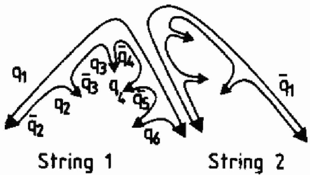
Figure 2: string fragmentation

II.2 Cluster Fragmentation Model

The Cluster Fragmentation Model has been proposed by WolframWolfram1980 in 1980. Webber Cluster Fragmentation Model(WCFM)Webber-cluster is the well-known example. It has three parts:

• The formation of color-singlet cluster. Gluons split into quark pairs after parton shower: $g\rightarrow q\bar{q}$. Adjacent quark and anti-quark from different gluons combine to form a color-singlet.

• Cluster with large invariant mass fragments into smaller ones.

• Little cluster decays into primary hadrons.i.e., $Cluster\rightarrow hadron1+hadron2$.

Note that only two-body decay or fragmentation is adopted in the Webber cluster fragmentation model. The corresponding hadronization picture is local, universal and simple. Its fragmentation picture is shown in Fig. 3.

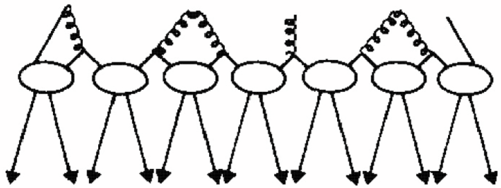
Figure 3: cluster fragmentation

II.3 Quark Combination Model

In the framework of SDQCM, Quark Production Rule(QPR), Quark Combination Rule (QCR) are adopted to describe the hadronization in a color singlet system, and then a simple Longitudinal Phase Space Approximation (LPSA) is used to obtain the momentum distribution for primary hadrons in its own system. Finally this hadronization scheme is extended to the multi-parton states. Here we briefly introduce the SDQCM and list the relevant equations(for detail, see ref. Xie2 ; Si:1997zs ).

II.3.1 QPR and QCR for $q\bar{q}$ system

In a color singlet system formed by $q\bar{q}$, $N$ pairs of quarks can be produced by vacuum excitation via strong interaction. We assume that $N$ satisfies Poisson Distribution:

$$P(<N>,N-1)={<N>^{N-1}\over(N-1)!}e^{-<N>}$$ (2)

where $<N>$ is the average number of those quark pairs. According to QPR, $<N>$ is given by

$$<N>=\sqrt{\alpha^{2}+\beta(W-{{M}_{q}}-{{M}_{\bar{q}}}+2\bar{m})}-\alpha-1,~{}~{}~{}~{}~{}\\ \alpha=\beta\bar{m}-{{1}\over{4}}$$ (3)

where $W$ is the invariant mass of the system, $\beta$ is a free parameter, $\bar{m}$ is the average mass of newborn quarks, and $M_{q}$ and $M_{\bar{q}}$ are the masses of endpoint quark and anti-quark. Thus we have $N$ pairs of quarks according to eqs. (2), (3) (containing one primary quark pair).

When describing how quarks and antiquarks form hadrons, we find that all kinds of hadronization models satisfy the near correlation in rapidity more or less. Since there is no deep understanding of the significance and the role of this, the near rapidity correlation has not been used sufficiently. In ref. Xie1 , we have shown that the nearest correlation in rapidity is in agreement with the fundamental requirements of QCD, and determines QCR completely. The rule guarantees that the combination of quarks across more than two rapidity gaps never emerges and that $N$ quarks and $N$ antiquarks are exactly exhausted, which guarantees the unitarity (see ref. Han:2009jw ). Given that the quarks and antiquarks are stochastically arranged in rapidity space, each order can occur with the same probability. Then the probability distribution for $N$ quarks and $N$ antiquarks to combine into $M$ mesons, $B$ baryons and $B$ anti-baryons according to QCR is given by

$${X_{MB}=}{{2N(N!)^{2}(M+2B-1)!}\over{(2N)!M!(B!)^{2}}}3^{M-1}\delta_{N,M+3B}$$ (4)

The average numbers of primary mesons $M(N)$ and baryons $B(N)$ are

$$\left\{\begin{array}[]{l}M(N)=\sum\limits_{M,B}MX_{MB}(N)\\ B(N)=\sum\limits_{M,B}BX_{MB}(N)\end{array}\right.$$ (5)

Approximately, in the combination for $N\geq 3$, $M(N)$ and baryons $B(N)$ can be well parameterized as linear functions of quark number $N$,

$$\left\{\begin{array}[]{l}M(N)=aN+b\\ B(N)={{(1-a)}\over 3}N-{b\over 3}\end{array}\right.$$ (6)

where $a=0.66$ and $b=0.56$. But for $N<3$, one has

$$M(N)=N,~{}~{}~{}~{}B(N)=0~{}~{}~{}~{}for~{}~{}~{}N<3$$ (7)

So that, the production ratio of baryon to meson is obtained from eqs. (5) and (6)

$${R_{B/M}=}{{(1-a)N-b}\over{3(aN+b)}}$$ (8)

We see that SDQCM treats meson and baryon formation uniformly, and there is no extra $ad~{}hoc$ mechanism and free parameters for the baryon production. Here the $B/M$ ratio is completely determined at a certain $N$, unlike in LSFM it is completely uncertain and has to be adjusted by free parameters, i.e, the ratio of diquark to quark ${qq}/q$.

II.3.2 momentum distribution of primary hadrons in the $q\bar{q}$ system

In order to give the momentum distribution of primary hadrons, each phenomenological model must have some inputs. For example, in LSFM, they use a symmetric longitudinal fragmentation function

$$f(z)\propto{{(1-z)^{a}}\over{z}}exp(-b{m_{T}^{2}\over z})$$ (9)

where $a$ and $b$ are two free parameters (and $a$ is flavor dependent). In this paper, in order to give the momentum distribution of primary hadrons produced according to QPR and QCR, we simply adopt the widely used LPSA which is equivalent to the constant distribution of rapidity. Hence a primary hadron $i$ is uniformly distributed in the rapidity axis, and then its rapidity can be written as

$$Y_{i}=Z+\xi_{i}Y,~{}~{}~{}~{}0\leq\xi_{i}\leq 1,$$ (10)

where $\xi_{i}$ is a random number; $Z$ and $Y$ are two arguments, and can be determined by energy-momentum conservation in such a color singlet system

$${\sum\limits_{i=1}^{H}}E_{i}=W,~{}~{}~{}~{}{\sum\limits_{i=1}^{H}}P_{Li}=0,$$ (11)

where $E_{i}$ and $P_{Li}$ denote the energy and the longitudinal momentum of the $i$th primary hadron respectively, obtained by

$$\left\{\begin{array}[]{ll}E_{i}=m_{Ti}{{exp(Y_{i})+exp(-Y_{i})}\over{2}}\\ P_{Li}=m_{Ti}{{exp(Y_{i})-exp(-Y_{i})}\over{2}}\end{array}\right.$$ (12)

where $m_{Ti}$ is given by

$$m_{Ti}=\sqrt{m_{i}^{2}+{\stackrel{{\scriptstyle\rightarrow}}{{P}}_{Ti}}^{2}}$$ (13)

where $m_{i}$ is the mass of the $i$th primary hadron, and $\stackrel{{\scriptstyle\rightarrow}}{{P}}_{Ti}$ obeys the distribution

$$f({\stackrel{{\scriptstyle\rightarrow}}{{P}}_{T1}},\ldots,{\stackrel{{\scriptstyle\rightarrow}}{{P}}_{TH}})\propto{\prod\limits_{i=1}^{H}}exp(-{{{\stackrel{{\scriptstyle\rightarrow}}{{P}}_{Ti}}^{2}}\over{\sigma^{2}}})\delta({\sum\limits_{i=1}^{H}}{\stackrel{{\scriptstyle\rightarrow}}{{P}}_{Ti}})$$ (14)

In this paper, we set $\sigma=0.2~{}GeV$. Eq. (14) is just what LSFM uses.

Note that LPSA or the constant rapidity distribution is rather naive, but it is convenient for us to study the correlations without introducing many complicating parameters.

II.3.3 hadronization of a multi-parton state

At the end of parton showering, a final multi-parton state will start to hadronize. To connect the final multi-parton state with SDQCM, we adopt a simple treatment assumed in WCFM, i.e. before hadronization, each gluon at last splits into a $q^{\prime}\bar{q^{\prime}}$ pair, the $q^{\prime}$ and $\bar{q^{\prime}}$ carry one half of the gluon momentum, and each of them forms a color singlet with their counterpart antiquark and quark in their neighbourhood, respectively. Now take the three parton state $q\bar{q}g$ as an example to illustrate the hadronization of a multi-parton state. Denote the 4-momenta for $q$, $\bar{q}$, $g$ as

$$P_{1}=(E_{q},{\stackrel{{\scriptstyle\rightarrow}}{{P}}_{q}}),~{}~{}P_{2}=(E_{g},{\stackrel{{\scriptstyle\rightarrow}}{{P}}_{g}}),~{}~{}P_{3}=(E_{\bar{q}},{\stackrel{{\scriptstyle\rightarrow}}{{P}}_{\bar{q}}}).$$ (15)

Before hadronization, the gluon splits into a $q^{\prime}\bar{q^{\prime}}$ pair and the $q^{\prime}$ and $\bar{q^{\prime}}$ carry one half of the gluon momentum, and the $q\bar{q}g$ system forms two color singlet subsystems $q\bar{q^{\prime}}$ and $q^{\prime}\bar{q}$. The invariant masses of the subsystems are

$$\left\{\begin{array}[]{lll}W_{q{\bar{q^{\prime}}}}=&\sqrt{(P_{1}+{{P_{2}}\over{2}})^{2}}=&\sqrt{(E_{q}+{{E_{g}}\over{2}})^{2}-({\stackrel{{\scriptstyle\rightarrow}}{{P}}_{q}}+{{\stackrel{{\scriptstyle\rightarrow}}{{P}}_{g}}\over{2}})^{2}}\\ W_{{q^{\prime}}{\bar{q}}}=&\sqrt{(P_{3}+{{P_{2}}\over{2}})^{2}}=&\sqrt{(E_{\bar{q}}+{{E_{g}}\over{2}})^{2}-({\stackrel{{\scriptstyle\rightarrow}}{{P}}_{\bar{q}}}+{{\stackrel{{\scriptstyle\rightarrow}}{{P}}_{g}}\over{2}})^{2}}\end{array}\right.$$ (16)

As was commonly argued by Sjöstrand and Khoze recentlykhoze , the confinement effects should lead to a subdivision of the full $q\bar{q}$ system into color singlet subsystems with screened interactions between these subsystems $q\bar{q^{\prime}}$ and $q^{\prime}\bar{q}$. Hence SDQCM can be applied independently to each color singlet subsystem,i.e., we can apply the equations in the former two subsections to each subsystem, and obtain the momentum distribution for the primary hadrons in their own center-of-mass system. Then after Lorentz transformation, the momentum distribution of the primary hadrons in laboratory frame is given. This treatment can be extended to a general multi-parton state, for example, see Fig. 4.

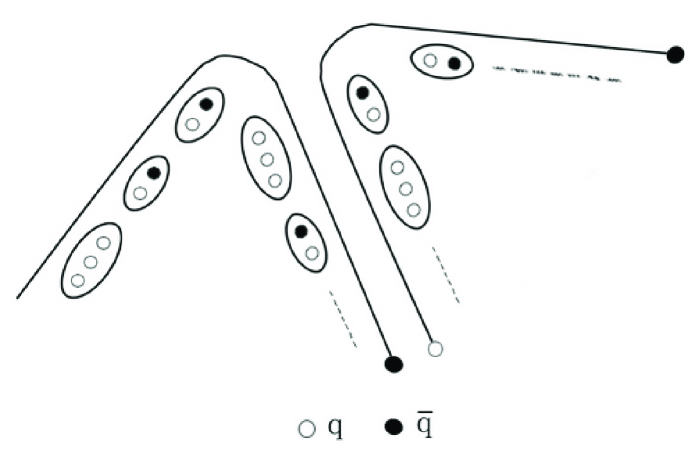
Figure 4: quark combination

Obviously, when the emitting gluon is soft or collinear with the direction of $q$ or $\bar{q}$, $q\bar{q}g$ cannot be distinguished from $q\bar{q}$ and $W_{q\bar{q}^{\prime}}$ or $W_{q^{\prime}\bar{q}}$ is too small for hadronization. For the avoidance of these situations, a cut-off mass $M_{min}$ has to be introduced. Here $M_{min}$ is a free parameter in the perturbative phase. Its value and energy dependence is theoretically uncertain. The physical assumption is that $M_{min}$ is independent of energyMattig ; sjostrand .

III Results and Discussion

In this paper, we study the hadronization process at $Z^{0}$ factory by LSFM and SDQCM. We focus on investigating the properties of the heavy hadrons, e.g., the ratio of baryon to meson and the baryon-antibaryon correlations. For LSFM, we use the default parameter values in PYTHIA, while for SDQCM, we adopt the parameters used in ref. Si:1997zs which fit data quite well.

The final hadron multiplicity at high energy $e^{+}e^{-}$ reactions is always an important topic. We list the predictions of final hadron multiplicities at $Z^{0}$ factory($\sqrt{S}=91.2GeV$) by LSFM and SDQCM in table I. The results of LSFM are obtained by running PYTHIA6.4 with the default parameters. The experimental data are from ref. pdg . It is found that the predictions of LSFM and those of SDQCM are consistent with most of the experimental data. However, the multiplicity of the heavy baryons, eg., $\Xi_{b}$, $\Sigma_{b},~{}\Omega_{b}$, are still not measured at $Z^{0}$ energy, and the corresponding theoretical predictions obtained by LSFM and SDQCM are quite different. Therefore it is important to measure their production rates at $Z^{0}$ pole in order to discriminate different hadronization mechanisms. At the $Z^{0}$ energy, we study the relation between the integrated luminosity and the producing number of the heavy baryons. The corresponding results are displayed in Fig.5. It is obvious that for the LEP I, the production number for $\Xi_{b}$ predicted by LSFM(SDQCM) is about $10^{3}$, and that for $\Omega_{b}$ is several tens(hundreds). In order to study the heavy baryon production mechanism with enough precision, the integrated luminosity should be increased as large as possible. For example, if the integrated luminosity of $Z^{0}$ factory can reach about $10^{4}pb^{-1}$, the produced number of $\Omega_{b}$ may reach several thousands(ten thousands) according to the prediction of LSFM(SDQCM), which makes it possible to study the properties of the heavy baryons and to test the hadronization models with higher precision.

Table 1: Results for average hadron multiplicities at $Z^{0}$ factory. The experimental data are from ref. pdg .

Particle	EXP DATA	LSFM	SDQCM
$\pi^{+}$	17.02 $\pm$0.19	17.125	17.766
$\pi^{0}$	9.42 $\pm$0.32	9.696	9.633
$K^{+}$	2.228 $\pm$0.059	2.312	2.145
$K^{0}$	2.049 $\pm$0.026	2.079	1.758
$\eta$	1.049 $\pm$0.080	1.013	0.787
$D^{+}$	0.175 $\pm$0.016	0.166	0.217
$D^{0}$	0.454 $\pm$0.030	0.495	0.476
$B^{+}$	0.178 $\pm$0.006	0.174	0.182
$B^{0}$	0.165 $\pm$0.026	0.173	0.182
$B_{s}^{0}$	0.057 $\pm$0.013	0.052	0.053
$\omega$	1.016 $\pm$0.026	1.369	1.809
$\rho^{0}$	1.231 $\pm$0.065	1.524	1.842
$K^{*+}$	0.715 $\pm$0.059	1.112	1.043
$K^{*0}$	0.738 $\pm$0.024	1.107	1.012
$D^{*+}$	0.1937 $\pm$0.0057	0.2399	0.2547
$D^{*0}$	—	0.2407	0.2603
$p$	1.050 $\pm$0.032	1.223	0.928
$\Lambda$	0.3915 $\pm$0.0065	0.3930	0.4368
$\Sigma^{0}$	0.076 $\pm$0.011	0.075	0.135
$\Sigma^{-}$	0.081 $\pm$0.010	0.069	0.114
$\Sigma^{+}$	0.107 $\pm$0.011	0.074	0.122
$\Lambda_{c}^{+}$	0.078 $\pm$0.017	0.060	0.076
$\Lambda_{b}^{0}$	0.031 $\pm$0.016	0.035	0.044
$\Sigma_{c}^{0}$	—	0.0017	0.0073
$\Sigma_{b}^{0}$	—	0.0019	0.0102
$\Xi_{b}^{0}$	—	0.0024	0.0065
$\Omega_{b}^{-}$	—	0.00006	0.0008

Figure 5: The relation between integrated luminosity and the production number of heavy bayons at $Z^{0}$ energy. The lower solid line stands for the total luminosity of LEP I from 1993 to 1995 at energies around the $Z^{0}$ Abbiendi:1999zx .

We also show the results for the momentum distribution of $\pi^{\pm}$, $K^{\pm}$ and $p\bar{p}$ in Fig.6. The results of LSFM are more consistent than SDQCM. This is easy to understand, since SDQCM does not include any complicated inputs for the hadron momentum distributions to be improved in the future.

Figure 6: The momenta spectrum of $\pi^{\pm}$, $K^{\pm}$ and $p\bar{p}$ at $Z^{0}$ factory. Solid(dashed) line is for LSFM(SDQCM), and here $P_{beam}=\sqrt{S}/2$. The experimental data is from ref. OPAL .

The following focuses on studying the baryon to meson ratio and $B\bar{B}$ correlations which reflect the hadronization mechanism more directly. In LSFM, the baryon to meson ratios can be tuned by the free parameters, e.g., $qq/q$, $BM\bar{B}/(B\bar{B}+BM\bar{B})$. SDQCM describes the baryon and meson production in the uniform scheme, so that these ratios are obtained naturally. Some of these ratios are listed in table II at $Z^{0}$ factory. One can notice that both LSFM and SDQCM can explain the present data. In $e^{+}e^{-}$ annihilations, most baryons are produced directly, even if they are the decay products. They carry the main properties of their mother particles.

Table 2: Results for baryon to meson ratios at $Z^{0}$ factory. The experimental data are from ref. pdg .

	EXP DATA	LSFM	SDQCM
$\frac{\Lambda_{b}^{0}}{B^{0}}$	0.188 $\pm$0.101	0.201	0.239
$\frac{\Lambda_{b}^{0}}{B^{+}}$	0.174 $\pm$0.090	0.200	0.240
$\frac{\Lambda_{c}^{+}}{D^{0}}$	0.172 $\pm$0.039	0.121	0.160
$\frac{\Lambda_{c}^{+}}{D^{+}}$	0.446 $\pm$0.105	0.360	0.351

Studying the properties of baryons, especially the $B\bar{B}$ flavor correlations, is helpful to reveal the hadronic mechanism. Here the $B\bar{B}$ flavor correlation strength is defined as

$$R_{B\bar{B}}=N\frac{n_{pair}}{n_{B}+n_{\bar{B}}}$$

where $n_{pair}$ is the number of the $B\bar{B}$ pairs and $N_{B}(N_{\bar{B}})$ is the baryon(antibaryon) number. $N=2(1)$ in the case of $B=\bar{B}$($B\neq\bar{B}$)OPAL . The predictions of baryon antibaryon flavor correlation strength by SDQCM and LSFM are listed in table III together with the corresponding OPAL dataOPAL . The understanding of hadronization mechanism related to the heavy hadron production requires more precise measurements at the future $Z^{0}$ factory.

Table 3: Predictions of baryon antibaryon flavor correlations by SDQCM and LSFM, and the experimental results are from OPAL collaborationOPAL .

	EXP DATA	LSFM	SDQCM
$\Lambda\bar{\Lambda}$	0.49 $\pm$0.06	0.38	0.48
$\Xi^{-}\bar{\Xi}^{+}$	0.04 $\pm$0.06	0.14	0.15
$\Xi^{-}\bar{\Lambda}+\bar{\Xi}^{+}\Lambda$	0.463 $\pm$0.099	0.510	0.538
$\Lambda_{b}^{0}\bar{\Lambda}_{b}^{0}$	—	0.08	0.12

IV Summary and Outlook

In the $e^{+}e^{-}\to\gamma^{\ast}/Z^{0}\to h^{\prime}$ process, the final particles have no relations with the structure of the initial particles, so it is convenient to study the hadronization mechanism. Above all, such studies help to investigate the multi-production processes in other high energy reactions(e.g., at RHIC energy). In this paper, we report the predictions especially related to heavy hadrons, for example, baryon to meson ratio and $B\bar{B}$ flavor correlations obtained by LSFM and SDQCM in the hadronic $Z^{0}$ decay. These results show that the future experiments at $Z^{0}$ factory to test hadronization mechanism, especially rare hadronized events, such as the doubly heavy baryon production, are significant.

Though many studies have been made for the $e^{+}e^{-}\to h^{\prime}s$ process, still a lot of unclear but important topics are worth studying, such as the color connection effectsxsl . The color connection among final partons plays a crucial role in the surface between PQCD phase and the hadronization one(see Fig. 1). Different choices of the color connections of the final multi-parton system leads to different hadronization results. Recently, the doubly heavy baryon(e.g., $\Xi_{cc}$) production has been investigated in different reactionsms . In $e^{+}e^{-}$ annihilation, the doubly heavy baryon production reveals a special kind of color connection of the final parton system $q_{1}\bar{q}_{1}q_{2}\bar{q}_{2}+ng$($n\leq 0$). This kind of color connection has not been considered in the popular hadronization models. In ref. hanwei , the hadronization effects of this kind of color connection are investigated in an extremely limited case of $e^{+}e^{-}\to c\bar{c}q\bar{q}\to h^{\prime}s$ process at $B$ factory energies. There cq and $\bar{c}\bar{q}$ form diquark-antidiquark pair, which is treated as a color singlet string and fragments into hadrons in the framework of LSFM. However due to the phase space limitation, the hadronization effect induced by diquark pair fragmentation is small. Fortunately, in the future $Z^{0}$ factory, a large number of events such as $e^{+}e^{-}\to Z^{0}\to\Xi_{cc}\bar{c}\bar{c}X$ will be producedzhangzx , so that the correlated physical observables can be measured with higher statistics. As a result, the hadronization mechanism and the related non-perturbative nature can be well studied at $Z^{0}$ pole energy.

References

- (1) T. Sjöstrand, Inter. J. of Mod. Phys. A 3, 751 (1988).
- (2) S. Wolfram, in: Proc. 15th Recontre de Moriond (1980) ed. J. Iran Thanh Van.
- (3) G. Marchesini and B. R. Webber, Nucl. Phys. B 238, 1 (1984); B. R. Webber, Nucl. Phys. B 238, 492 (1984).
- (4) Adler SS et al., Phys. Rev. Lett. 91, 172301 (2003).
- (5) Adams J et al., arXiv:nucl-ex/0601042; Long H, J. Phys. G 30, 193 (2004).
- (6) S. S. Adler et al. [PHENIX Collaboration], Phys. Rev. Lett. 91, 182301 (2003); J. Adams et al. [STAR Collaboration], Phys. Rev. Lett. 92, 052302 (2004); J. Adams et al. [STAR Collaboration], Phys. Rev. Lett. 95, 122301 (2005).
- (7) R. C. Hwa and C. B. Yang, Phys. Rev. C 67, 034902 (2003).
- (8) R. J. Fries, B. Muller, C. Nonaka and S. A. Bass, Phys. Rev. Lett. 90, 202303 (2003).
- (9) V. Greco, C. M. Ko and P. Levai, Phys. Rev. Lett. 90, 202302 (2003).
- (10) F. L. Shao, Q. B. Xie and Q. Wang, Phys. Rev. C 71, 044903 (2005); T. Yao, Q. B. Xie and F. L. Shao, Chinese Physics C 32, 356 (2008); T. Yao, W. Zhou and Q. B. Xie, Phys. Rev. C 78, 064911 (2008).
- (11) V. V. Anisovich and V. M. Shekhter, Nucl. Phys. B 55, 455 (1973); J. D. Bjorken and G. R. Farrar, Phys. Rev. D 9, 1449 (1974).
- (12) TASSO Collab., M. Althoff et al., Z. Phys. C 17, 5 (1983).
- (13) Qu-Bing Xie, in Proceedings of the XIXth International Symposium on Multi-particle Dynamics 1988, edited by D. Schiff and J. Tran Thanh Van (World Scientific, Singapore 1988), P. 369, and the references therein.
- (14) H. . Fang, High Energy Phys. Nucl. Phys. 13, 886 (1989).
- (15) Z. G. Si, Q. B. Xie and Q. Wang, Commun. Theor. Phys. 28, 85 (1997); Z. G. Si and Q. B. Xie, High Ener. Phys. and Nucl. Phys. 23, 445 (1999)(in Chinese).
- (16) X. Artru and G. Mennessier, Nucl. Phys. B 70, 93 (1974).
- (17) N. K. Glendenning and T. Matsui, Phys. Rev. D 28, 2890 (1983).
- (18) T. Schenfeld, B. Muller, K. Sailer, J. Reinhardt, W. Greiner and A. Schafer, Phys. Lett. B 247, 5 (1990).
- (19) H. P. Pavel and D. M. Brink, Z. Phys. C 51, 119 (1991).
- (20) G. Gustafson, Z. Phys. C 15, 155 (1982).
- (21) Qu-Bing Xie and Xi-Ming Liu, Phys. Rev. D 38, 2169 (1988).
- (22) W. Han, S. Y. Li, Y. H. Shang, F. L. Shao and T. Yao, Phys. Rev. C 80, 035202 (2009).
- (23) T. Sjöstrand and V. A. Khoze, Z. Phys. C 62, 281 (1994).
- (24) P. Mättig, Phys. Rep. 177, 141 (1989).
- (25) Particle Data Group, Phys. Lett. B 667, 355 (2008).
- (26) G. Abbiendi et al. [OPAL Collaboration], Eur. Phys. J. C 14, 373 (2000).
- (27) OPAL Collab., P. D. Acton, et al., Phys. Lett. B 305, 415 (1993).
- (28) F. L. Shao, Q. B. Xie, S. Y. Li and Q. Wang, Phys. Rev. D 69, 054007 (2004); Y. Jin, Q. B. Xie, and S. Y. Li, High Ener. Phys. and Nucl. Phys. 27, 282 (2003)(in Chinese); S. Y. Li, F. L. Shao, Q. B. Xie and Q. Wang, Phys. Rev. D 65, 077503 (2002); F. L. Shao and Q. B. Xie, High Ener. Phys. and Nucl. Phys. 25, 710 (2001)(in Chinese); Q. Wang, G. Gustafson, Y. Jin, and Q. B. Xie, Phys. Rev. D 64, 012006 (2001); Q. Wang, G. Gustafson, and Q. B. Xie, Phys. Rev. D 62, 054004 (2000); S. Y. Li, Z. G. Si, Q. B. Xie and Q. Wang, Phys. Lett. B 458, 370 (1999); Z. G. Si, and Q. B. Xie, High Energy Phys. Nucl. Phys. 22, 307 (1998)(in Chinese); Z. G. Si, Q. Wang and Q. B. Xie, Phys. Lett. B 401, 107 (1997); L. L. Tian, Q. B. Xie and Z. G. Si, High Energy Phys. Nucl. Phys. 17, 147 (1993); L. L. Tian, Q. B. Xie and Z. G. Si, Phys. Rev. D 49, 4517 (1994).
- (29) J. P. Ma and Z. G. Si, Phys. Lett. B 568, 135 (2003); S. Y. Li, Z. G. Si and Z. J. Yang, Phys. Lett. B 648, 284 (2007); C. H. Chang, J. P. Ma, C. F. Qiao and X. G. Wu, J. Phys. G 34, 845 (2007); B. Aubert et al. [BABAR Collaboration], Phys. Rev. D 74, 011103 (2006).
- (30) Wei Han, Shi-Yuan Li, Zong-Guo Si and Zhong-Juan Yang, Phys. Lett. B 642, 62 (2006).
- (31) Chao-Hsi Chang, Jian-Xiong Wang, et al., in this volume.