Supersymmetries of the spin-$1/2$ particle in the field of magnetic vortex, and anyons

Abstract

The quantum nonrelativistic spin-$1/2$ planar systems in the presence of a perpendicular magnetic field are known to possess the $N=2$ supersymmetry. We consider such a system in the field of a magnetic vortex, and find that there are just two self-adjoint extensions of the Hamiltonian that are compatible with the standard $N=2$ supersymmetry. We show that only in these two cases one of the subsystems coincides with the original spinless Aharonov-Bohm model and comes accompanied by the super-partner Hamiltonian which allows a singular behavior of the wave functions. We find a family of additional, nonlocal integrals of motion and treat them together with local supercharges in the unifying framework of the tri-supersymmetry. The inclusion of the dynamical conformal symmetries leads to an infinitely generated superalgebra, that contains several representations of the superconformal $osp(2|2)$ symmetry. We present the application of the results in the framework of the two-body model of identical anyons. The nontrivial contact interaction and the emerging $N=2$ linear and nonlinear supersymmetries of the anyons are discussed.

1 Introduction

It is well known that a non-relativistic planar system of a spin-$1/2$ particle of gyromagnetic ratio $g=2$ in the presence of an external perpendicular magnetic field $\vec{B}=B_{3}(x_{1},x_{2})\hat{x}_{3}$ possesses $N=2$ supersymmetry [1, 2, 3]. Its dynamics is described by the Pauli Hamiltonian

$$\mathcal{H}=\frac{1}{2m}\sum_{j=1,2}\mathcal{P}^{2}_{j}-\frac{e\hbar}{2mc}B_{3}\,\sigma_{3}\,,$$ (1.1)

where $\mathcal{P}_{j}=-i\hbar\partial_{j}-\frac{e}{c}A_{j}$, $B_{3}=\partial_{1}A_{2}-\partial_{2}A_{1}$, that can be presented as a perfect square 

$$\mathcal{H}=Q_{1}^{2}\,,\qquad Q_{1}=\sum_{j=1,2}\mathcal{P}_{j}\sigma_{j}\,.$$ (1.2)

The $Q_{1}$ is therefore an integral of motion. The spin $s_{3}=\frac{1}{2}\sigma_{3}$ is another conserved quantity. Due to relations $\sigma_{3}^{2}=1$ and $\{\sigma_{3},Q_{1}\}=0$, the $\Gamma=\sigma_{3}$ can be considered as the $\mathbb{Z}_{2}$-grading operator, while $Q_{1}$ can be treated as a fermionic supercharge. Another supercharge is then defined as

$$Q_{2}=i\sigma_{3}Q_{1}=\epsilon_{ij}\mathcal{P}_{i}\sigma_{j}=\mathcal{P}_{1}\sigma_{2}-\mathcal{P}_{2}\sigma_{1}\,.$$ (1.3)

The $Q_{a}$, $a=1,2$, and $\mathcal{H}$ generate the $N=2$ superalgebra graded by $\sigma_{3}$,

$$\{Q_{a},Q_{b}\}=2\delta_{ab}\mathcal{H}\,,\qquad[Q_{a},H]=0\,,\qquad\{\sigma_{3},Q_{a}\}=[\sigma_{3},\mathcal{H}]=0\,.$$ (1.4)

The described algebraic procedure applies to the case of any external field $B_{3}(x_{1},x_{2})$. For the simplest case of a homogeneous magnetic field, the supersymmetry provides with a natural explanation of the degeneracy of the Landau levels [4], and it is essential in the understanding of the quantum Hall effect [5].

The procedure outlined in (1.2)–(1.4) is quite formal, however, and can miss some important subtleties related to the domains of the involved supersymmetry generators.

In the present paper we focus on investigation of the supersymmetry and its conformal extension for a non-relativistic electron in the presence of a magnetic vortex. This corresponds to the Aharonov-Bohm (AB) effect for the spin-$1/2$ particle system, in which the indicated subtleties play a crucial role.

The field in the case of interest is produced by an infinitely thin solenoid of infinite length that punctures the plane at $x_{1}=x_{2}=0$. The electromagnetic potential in the symmetric gauge reads

$$\vec{A}=\frac{\Phi}{2\pi}\left(-\frac{x_{2}}{x_{1}^{2}+x_{2}^{2}},\frac{x_{1}}{x_{1}^{2}+x_{2}^{2}},0\right)=\frac{\Phi}{2\pi r}\left(-\sin\varphi\,,\ \cos\varphi\,,0\right)\,,$$ (1.5)

where $x_{1}=r\cos\varphi,\ x_{2}=r\sin\varphi$, $-\pi<\varphi\leq\pi$, and $\Phi$ is the flux of the singular magnetic field, $B_{3}=\Phi\,\delta^{2}(x_{1},x_{2})$. Corresponding Hamiltonian is

$$\mathcal{H}_{\alpha}=-\partial^{2}_{r}-\frac{1}{r}\partial_{r}+\frac{1}{r^{2}}(-i\partial_{\varphi}+\alpha)^{2}+\alpha\frac{1}{r}\delta(r)\sigma_{3}\,,\quad\alpha=\frac{1}{2\pi}\Phi\,,$$ (1.6)

where we use the identity $\delta^{2}(x_{1},x_{2})=\frac{1}{\pi r}\delta(r)$ for the two dimensional Dirac delta function.

The (spinless) model was introduced by Aharonov and Bohm in a seminal work [6], where they demonstrated the significance of the electromagnetic potential in quantum mechanics. It is this setting that was used in the dynamical realization of anyons [7], [8]. The relativistic modification of the system appears in the study of the cosmic strings [9], [10], the topological defects which are supposed to appear in the early universe. Nowadays, the AB effect attracts much attention in the physics of graphene and nanotubes [11].

In two dimensions, the Dirac delta term in (1.6) is not, however, defined uniquely [12]. The system can be specified unambiguously as soon as the domain of the Hamiltonian (1.6) is fixed [13] . Different choices of the domain lead then to different physical systems. Distinct physical properties are usually attributed to the variation of the hidden characteristics of the magnetic flux within the vortex [14]. Here, we identify and analyze the systems described by (1.6), for which the procedure (1.2)–(1.4) is consistent.

The paper is organized as follows. In the next Section, we find the proper domain of the operators $Q_{1}$ and $Q_{2}=i\sigma_{3}Q_{1}$ in order to identify which kind of AB Hamiltonians allows a physical supersymmetric structure. We will see that the physically acceptable Hamiltonians with supersymmetry obligatorily involve non trivial self-adjoint extensions. So far this crucial point was not discussed appropriately in the broad literature on the AB problem and supersymmetry [15], [16], [17]. In Section 3, we identify additional nonlocal integrals of motion, and analyze the associated hidden supersymmetry and related extended supersymmetric structure in the form of tri-supersymmetry [18], [19]. The incorporation of the conformal symmetry into the framework of the tri-supersymmetry is considered in Section 4. We apply the results to the theory of anyons in Section 5. There, the two-body systems of the interacting anyons are discussed in the light of the superalgebraic structure revealed in the preceding sections. In particular, the $N=2$ nonlinear supersymmetry of the two-body anyonic model is presented. The last Section is devoted to the discussion of the results.

2 $N=2$ supersymmetry

In the forthcoming analysis of the system, the magnetic flux will be restricted to the interval $\alpha\in[0,1)$. This can be done without loss of generality as the systems with the fluxes $\alpha$ and $\alpha+n$ for integer $n$ can be related by the unitary transformation,

$$\mathcal{H}_{\alpha+n}=U_{n}^{-1}\mathcal{H}_{\alpha}U_{n},\quad U_{n}=e^{in\varphi}\,\mathds{1}\,,$$ (2.1)

where $\mathds{1}$ is the unit $2\times 2$ matrix.

The formal supercharge operator $Q_{1}$ of the Aharonov-Bohm system can be obtained directly by the substitution of (1.5) into (1.2). The explicit form of the $Q_{1}$ in polar coordinates,

$$Q_{1}=q_{+}\sigma_{+}+q_{-}\sigma_{-}\,,\qquad q_{\pm}=-ie^{\mp i\varphi}\left(\partial_{r}\pm\frac{1}{r}\left(-i\partial_{\varphi}+\alpha\right)\right),\quad\sigma_{\pm}=\frac{1}{2}(\sigma_{1}\pm i\sigma_{2})\,,$$ (2.2)

suggests that it preserves the subspaces $\mathfrak{H}_{l}$,

$$\mathfrak{H}_{l}=\left(\begin{array}[]{c}e^{il\varphi}\\ e^{i(l+1)\varphi}\end{array}\right)\otimes L_{2}(\mathbb{R}_{+},rdr),\qquad Q_{1}\mathfrak{H}_{l}\subset\mathfrak{H}_{l},\qquad l\in\mathbb{Z}\,.$$ (2.3)

The eigenvectors of the $Q_{1}$ are the states of fixed energy, see (1.2). Define the function $\Phi_{\lambda,l}(r,\varphi)=(e^{il\varphi}\phi_{\lambda,1}(r),e^{i(l+1)\varphi}\phi_{\lambda,2}(r))^{T}$, where $T$ means a transposition. The eigenvalue equation $Q_{1}\Phi_{\lambda,l}(r,\varphi)=\lambda\Phi_{\lambda,l}(r,\varphi)$ can be written equivalently as

$$\left[\partial_{r}+(l+\alpha+1)\frac{1}{r}\right]\phi_{\lambda,2}(r)=i\lambda\phi_{\lambda,1}(r)\,,\qquad\left[\partial_{r}-(l+\alpha)\frac{1}{r}\right]\phi_{\lambda,1}(r)=i\lambda\phi_{\lambda,2}(r)\,.$$ (2.4)

The general solution of (2.4) is given in terms of the Bessel functions of the first and of the second kinds. Consider the case of nonzero $\lambda$. The lower component of the eigenfunction $\Phi_{\lambda,l}(r,\varphi)$ is

$$\phi_{\lambda,2}(r)=C_{1}^{l}\mathcal{J}_{|l+\alpha+1|}(|\lambda|r)+C_{2}^{l}\mathcal{Y}_{|l+\alpha+1|}(|\lambda|r)\,.$$ (2.5)

The associated upper component depends on $\epsilon=sign\,(l+\alpha+1)$,

$$\phi_{\lambda,1}(r)=-i\epsilon\frac{\lambda}{|\lambda|}\left(C_{1}^{l}\mathcal{J}_{\epsilon(l+\alpha)}(|\lambda|r)+C_{2}^{l}\mathcal{Y}_{\epsilon(l+\alpha)}(|\lambda|r)\right).$$ (2.6)

The solutions are not square integrable. They are acceptable, however, in the sense of the scattering states (generalized wave functions) as long as their square integrability at the origin is maintained.

For $\alpha=0$, this condition fixes $C_{2}^{l}=0$ for all values of $l$. The wave functions $\Phi_{\lambda,l}$ are regular at the origin and the system can be identified with the free spin-$\frac{1}{2}$ particle in the plane. The domain of $\mathcal{H}_{0}$ is invariant with respect to $\sigma_{3}$, and the procedure (1.2)–(1.4) is consistent for the free-particle system.

We consider the case $\alpha\in(0,1)$ from now on if not stated otherwise. The condition of local square integrability fixes $C_{2}^{l}=0$ again as long as $l\neq-1$. However, for $l=-1$, the function $\Phi_{\lambda,-1}$ is square integrable for any values of the coefficients $C_{1}^{l}$ and $C_{2}^{l}$ with $l=-1$. This spoils its physical interpretation as the function cannot be fixed (up to an overall normalization) uniquely. To avoid this ambiguity, the behavior of the wave functions for $r\sim 0$ has to be specified. This, in turn, will fix the self-adjoint extension of the $Q_{1}$.

The operator $Q_{1}$ defined on the space of infinitely smooth two-component functions with compact support is symmetric. Using a standard theory of self-adjoint extensions of symmetric operators [20], we extend its domain by relaxing the regularity of the functions in the sector of two specific partial waves. The corresponding boundary conditions

$$\lim_{r\rightarrow 0^{+}}\Psi\sim\left(\begin{array}[]{l}(1+e^{i\gamma})2^{-\alpha}\Gamma(1-\alpha)r^{-1+\alpha}e^{-i\varphi}\\ (1-e^{i\gamma})2^{-1+\alpha}\Gamma(\alpha)r^{-\alpha}\end{array}\right)$$ (2.7)

specify the domain of the self-adjoint extensions $Q^{\gamma}_{1}$ of the $Q_{1}$ for $\alpha\in(0,1)$ that form a one-parameter family marked by $\gamma\in[0,2\pi)$.

Defining the Hamiltonian $\mathcal{H}^{\gamma}_{\alpha}=(Q_{1}^{\gamma})^{2}$, the operator $Q_{1}^{\gamma}$ satisfies the relations $[Q_{1}^{\gamma},\mathcal{H}^{\gamma}_{\alpha}]=0,\ \{Q_{1}^{\gamma},Q_{1}^{\gamma}\}=2\mathcal{H}_{\alpha}^{\gamma}$, and might be considered as a supercharge of the $N=1$ supersymmetry. The action of the operator $\sigma_{3}$ is not well defined, however, for generic values of $\gamma$; it preserves the boundary conditions (2.7) if and only if the parameter $\gamma$ acquires only two discrete values

$$\gamma=0,\,\pi\,.$$ (2.8)

For other values of $\gamma$, the $\sigma_{3}$ perturbs the relative coefficient between the up and down components of (2.7) and maps the wave functions out of the physical domain. In the two cases (2.8), the spin operator $s_{3}=\frac{1}{2}\sigma_{3}$ is a well defined physical observable that is a symmetry of the Hamiltonians

$$\mathcal{H}_{\alpha}^{\gamma=0}=\left(\begin{array}[]{cc}H_{\alpha}^{0}&0\\ \\ 0&H_{\alpha}^{AB}\\ \end{array}\right)\,,\qquad\qquad\mathcal{H}_{\alpha}^{\gamma=\pi}=\left(\begin{array}[]{cc}H_{\alpha}^{AB}&0\\ \\ 0&H_{\alpha}^{\pi}\\ \end{array}\right)\,,$$ (2.9)

$[s_{3},\mathcal{H}_{\alpha}^{\gamma}]=0$. These two Hamiltonians possess therefore the $N=2$ supersymmetry since the second supercharge $Q_{2}^{\gamma}=i\sigma_{3}Q_{1}^{\gamma}$ is defined consistently on the same domain as $Q_{1}^{\gamma}$. In accordance with (1.2), (1.3), the explicit matrix form of the supercharges is

$$Q_{1}^{\gamma}=\left(\begin{array}[]{cc}0&{\cal P}_{1}-i{\cal P}_{2}\\ {\cal P}_{1}+i{\cal P}_{2}&0\end{array}\right)\,,\qquad Q_{2}^{\gamma}=\left(\begin{array}[]{cc}0&{\cal P}_{2}+i{\cal P}_{1}\\ {\cal P}_{2}-i{\cal P}_{1}&0\end{array}\right).$$ (2.10)

Here, as in (2.9), for $\gamma=0$ and $\gamma=\pi$ the corresponding operators act on different domains.

The boundary conditions (2.7) acquire particularly simple form : for $\gamma=\pi$ the upper component disappears, while for $\gamma=0$ the lower one does. This enables a direct interpretation of the subsystem represented by $H_{\alpha}^{AB}$; it’s domain is free of the singular wave functions since the corresponding singular component in the boundary condition (2.7) vanishes for the specific choice of $\gamma$. In what follows, the Hamiltonian $H_{\alpha}^{AB}$ can therefore be identified with that of the spinless system studied originally by Aharonov and Bohm [6]. We shall stress that this subsystem appears only for (2.8). For other values of $\gamma$, the singular behavior is enforced in both, up- and down-, components of the wave functions, see (2.7).

The generator of rotations in the plane, the orbital angular momentum shifted by the flux,

$$J=x_{1}\mathcal{P}_{2}-x_{2}\mathcal{P}_{1}=-i\partial_{\varphi}+\alpha\,,$$ (2.11)

represents another symmetry since it commutes with (2.9) and preserves the boundary conditions (2.7) for $\gamma=0,\pi$. Hence, both systems (2.9) are rotationally invariant. Moreover, each subsystem $H^{AB}_{\alpha}$, $H_{\alpha}^{0}$ and $H^{\pi}_{\alpha}$ is rotationally invariant since $s_{3}$ is also the integrals of motion. Notice here that for the values of $\gamma$ different from (2.8), the operator $J$ would change the relative coefficient of the up- and down- components in (2.7), and would not preserve the domain of $Q_{1}^{\gamma}$. This should be interpreted as the absence of the rotational invariance for diagonal subsystems of the system $\mathcal{H}_{\alpha}^{\gamma}=(Q_{1}^{\gamma})^{2}$, $\gamma\neq 0,\pi$, caused by the inner characteristics of the magnetic flux. The total angular momentum $J+s_{3}$ would preserve, however, the boundary conditions (2.7) even for $\gamma\neq 0,\pi$, and would be an integral of motion of the $N=1$ supersymmetric family of the systems in which we are not interested anymore.

From now on, we will suppose that $\gamma$ acquires one of the two values specified in (2.8). In this case, both systems (2.9) are rotationally invariant, the spin is preserved, and they possess the $N=2$ supersymmetry. The subsystem $H^{AB}_{\alpha}$ coincides with the original Aharonov-Bohm setting.

We can find the common eigenvectors $\Psi_{E,l,s}^{\gamma}$ of $\mathcal{H}^{\gamma}_{\alpha}$, $s_{3}$ and $J$ marked by the energy $E$, the orbital angular momentum $l$ and the spin sign $s=\pm$,

$$\mathcal{H}_{\alpha}^{\gamma}\Psi_{E,l,s}^{\gamma}=E\Psi_{E,l,s}^{\gamma},\qquad J\Psi_{E,l,s}^{\gamma}=(l+\alpha)\Psi_{E,l,s}^{\gamma},\qquad s_{3}\Psi_{E,l,\pm}^{\gamma}=\pm\frac{1}{2}\Psi_{E,l,\pm}^{\gamma}\,.$$ (2.12)

Having in mind the relation $(Q_{1}^{\gamma})^{2}=\mathcal{H}_{\alpha}^{\gamma}$, these functions are obtained as linear combinations of $\Phi_{\lambda,l}$ and $\Phi_{-\lambda,l}$. The wave functions $\Psi_{E,l,s}^{\gamma}$ for $l\neq-1$ can be written as $\Psi_{E,l,+}^{\gamma}=\mathcal{J}_{|\alpha+l|}(\sqrt{E}r)e^{il\varphi}\,\mathbf{v}_{+}$ and $\Psi_{E,l+1,-}^{\gamma}=\mathcal{J}_{|\alpha+l+1|}(\sqrt{E}r)e^{i(l+1)\varphi}\,\mathbf{v}_{-}$ where $s_{3}\,\mathbf{v}_{\pm}=\pm\frac{1}{2}\,\mathbf{v}_{\pm}$. The partial waves in the subspace $\mathfrak{H}_{-1}$ have to obey the boundary conditions (2.7), which fix the coefficients in (2.5) and (2.6) in a unique way. Their explicit form is

$$\Psi_{E,-1,+}^{\pi}=\left(\mathcal{J}_{1-\alpha}(\sqrt{E}\,r)e^{-i\varphi},0\right)^{T},\qquad\Psi_{E,0,-}^{\pi}=\left(0,\,\mathcal{J}_{-\alpha}(\sqrt{E}\,r)\right)^{T},\qquad\gamma=\pi,$$ (2.13)

and

$$\Psi_{E,-1,+}^{0}=\left(\mathcal{J}_{-1+\alpha}(\sqrt{E}\,r)e^{-i\varphi},0\right)^{T},\qquad\Psi_{E,0,-}^{0}=\left(0,\,\mathcal{J}_{\alpha}(\sqrt{E}\,r)\right)^{T},\qquad\gamma=0\,.$$ (2.14)

To complete the analysis of the spectrum of $\mathcal{H}_{\alpha}^{\gamma}$, we present the zero energy wave functions. The partial waves with $l\neq-1$ are $\Psi^{\gamma}_{0,l,+}=r^{|l+\alpha|}e^{il\varphi}\,\mathbf{v}_{+}$ and $\Psi^{\gamma}_{0,l+1,-}=r^{|l+1+\alpha|}e^{i(l+1)\varphi}\,\mathbf{v}_{-}$ while the wave functions of zero energy from the subspace $\mathfrak{H}_{-1}$ acquire the form

$$\Psi_{0,-1,+}^{\gamma}=\left\{\begin{array}[]{lc}(r^{1-\alpha}e^{-i\varphi},0)^{T}\,,&\gamma=\pi\\ (r^{-1+\alpha}e^{-i\varphi},0)^{T}\,,&\gamma=0\end{array}\right.,\qquad\Psi_{0,0,-}^{\gamma}=\left\{\begin{array}[]{lc}(0,r^{-\alpha})^{T},&\gamma=\pi\\ (0,r^{\alpha})^{T},&\gamma=0\end{array}\right.,\quad E=0\,.$$ (2.15)

Finally, let us note that the wave functions $\Psi_{E,l,\pm}$ for all integer $l$ and non-negative $E$ form the basis of the Hilbert space.

Let us discuss now the action of the supercharges on the eigenstates $\Psi_{E,l,\pm}^{\gamma}$. By the action of the $Q_{1}^{\gamma}$, the spin-up and spin-down eigenstates of positive energy are interchanged and the angular momentum is altered,

$$Q_{1}^{\gamma}\Psi_{E,l,+}^{\gamma}\sim\Psi_{E,l+1,-}^{\gamma}\,,\qquad Q_{1}^{\gamma}\Psi_{E,l+1,-}^{\gamma}\sim\Psi_{E,l,+}^{\gamma}\,.$$ (2.16)

In this manner, the supercharge $Q_{1}^{\gamma}$ reflects the degeneracy within the subspaces $\mathfrak{H}_{l}$. Each of these subspaces contains two zero modes, $\Psi_{0,l,+}$ and $\Psi_{0,l+1,-}$, of the $\mathcal{H}_{\alpha}^{\gamma}$ ; however, only one of them is annihilated by $Q_{1}^{\gamma}$.

In conclusion of this Section, let us summarize the results. For non-integer values of $\alpha$, there are just two systems described either by $\mathcal{H}_{\alpha}^{0}$ or $\mathcal{H}^{\pi}_{\alpha}$, which possess the genuine $N=2$ supersymmetry. Only in these two cases, one of the subsystems, represented by $H^{AB}_{\alpha}$, coincides with the original spinless Aharonov-Bohm model and comes accompanied with the super-partner Hamiltonian which allows the singular behavior of the wave functions. When $\alpha$ acquires integer values, the studied model is unitary equivalent to the free electron in the plane and has the $N=2$ supersymmetry as well. To our best knowledge, the careful treatment of this kind seems to be missing in the literature.

In the next Section we will show that the described $N=2$ supersymmetry is just a piece of a remarkable mosaic of the rich supersymmetric structure that underlines the system.

3 Hidden supersymmetry and tri-supersymmetry

The diagonal components of $\mathcal{H}^{0}_{\alpha}$ and $\mathcal{H}^{\pi}_{\alpha}$, identified with one of $H^{AB}_{\alpha}$, $H^{0}_{\alpha}$ or $H^{\pi}_{\alpha}$, can be looked at as those describing the spinless systems in presence of the magnetic vortex. These spinless Hamiltonians possess $N=2$ hidden (bosonized) supersymmetry in terms of self-adjoint, nonlocal supercharges, see [21] . This observation makes it possible to define directly two new operators $\tilde{Q}_{1}$ and $\tilde{Q}_{2}$,

$$\tilde{Q}^{\gamma}_{1}=\left(\begin{array}[]{cc}\mathcal{P}_{1}+ie^{i\gamma}R\mathcal{P}_{2}&0\\ 0&\mathcal{P}_{1}-ie^{i\gamma}R\mathcal{P}_{2}\end{array}\right)\,,\qquad\quad\tilde{Q}^{\gamma}_{2}=iR\tilde{Q}_{1}^{\gamma}\,,$$ (3.1)

that are well defined on the domain of $Q_{1}^{\gamma}$ (we remind that $\gamma$ acquires one of the two values (2.8)). They are nonlocal due to the presence of the operator of rotations

$$R=e^{i\pi(J-\alpha)},\qquad R\varphi R=\varphi+\pi,\qquad R^{2}=1\,.$$ (3.2)

The operators (3.1) anti-commute with $R$ while the Hamiltonian commutes with this operator. The operators $\tilde{Q}_{1}$ and $\tilde{Q}_{2}$ satisfy the relation

$$\{\tilde{Q}_{a}^{\gamma},\tilde{Q}_{b}^{\gamma}\}=2\delta_{ab}\mathcal{H}_{\alpha}^{\gamma}\,,$$ (3.3)

and form an alternative representation of the $N=2$ supersymmetry. As the supercharges (3.1) originate from the hidden supersymmetry of the spinless AB systems, we call the operators (3.1) the supercharges of the hidden supersymmetry (3.3).

Let us briefly discuss the action of the supercharge $\tilde{Q}_{1}^{\gamma}$ on the eigenstates of $\mathcal{H}^{0}_{\alpha}$ ($\mathcal{H}^{\pi}_{\alpha}$). It is instructive to rewrite the diagonal component of (3.1) in the polar coordinates,

$$\mathcal{P}_{1}+ie^{i\gamma}R\mathcal{P}_{2}=-ie^{-i\varphi}\left(\partial_{r}+\frac{1}{r}J\right)\Pi_{+}^{\gamma}-ie^{i\varphi}\left(\partial_{r}-\frac{1}{r}J\right)\Pi_{-}^{\gamma}\,,\quad\Pi_{\pm}^{\gamma}=\frac{1}{2}(1\pm e^{i\gamma}R)\,,$$ (3.4)

where the operators $\Pi_{\pm}^{\gamma}$, are projectors for $\gamma=0\,,\pi$. A similar form for the component $\mathcal{P}_{1}-ie^{i\gamma}R\mathcal{P}_{2}$ is obtained from (3.4) by the substitution $R\rightarrow-R$. This suggests that both $\tilde{Q}_{1}^{\gamma}$ and $\tilde{Q}_{2}^{\gamma}$ preserve the subspaces $\tilde{\mathfrak{H}}_{kl}$ of the form

$$\tilde{\mathfrak{H}}_{kl}=\left\{f\,|\,f\in\left(\begin{array}[]{c}\{e^{i(2k-e^{i\gamma})\varphi},e^{i2k\varphi}\}\\ \{e^{i(2l+e^{i\gamma})\varphi},e^{i2l\varphi}\}\end{array}\right)\otimes L_{2}(\mathbb{R}^{+},rdr),\ k,\ l\in\mathbb{Z}\right\}.$$ (3.5)

Then the action of the supercharge $\tilde{Q}_{1}^{\gamma}$ on the wave functions $\Psi_{E,l,\pm}$ can be inferred directly and reads

$$\tilde{Q}_{1}^{\gamma}\Psi^{\gamma}_{E,2l,\pm}\sim\Psi^{\gamma}_{E,2l-1,\pm}\,,\qquad\tilde{Q}_{1}^{\gamma}\Psi_{E,2l-1,\pm}^{\gamma}\sim\Psi^{\gamma}_{E,2l,\pm}\,.$$ (3.6)

Considering the states of zero energy, the situation is qualitatively similar to the case of $Q_{1}^{\gamma}$. The Hamiltonian $\mathcal{H}^{0}_{\alpha}$ ($\mathcal{H}^{\pi}_{\alpha}$) has two spin-up and two spin-down zero modes in $\tilde{\mathfrak{H}}_{kl}$ and $\tilde{Q}_{1}^{\gamma}$ annihilates only half of them.

We pose the following question : is it possible to include both the local, $Q_{1}^{\gamma}$ and $Q_{2}^{\gamma}$, and nonlocal, (3.1), supercharges in the unifying scheme of an extended superalgebra? To respond it, we note that all the operators $Q_{a}^{\gamma}$ and $\tilde{Q}_{a}^{\gamma}$ ($a=1,2$) have vanishing either commutator or anti-commutator with each of the operators

$$\sigma_{3}\,,\qquad R\,,\qquad\sigma_{3}R\,.$$ (3.7)

Each of the operators (3.7) commutes with $\mathcal{H}^{\gamma}_{\alpha}$. Hence each is equally good candidate for the grading operator $\Gamma$ of the extended superalgebra, in which it should classify the integrals into bosonic and fermionic ones.

Let us choose

$$\Gamma=\sigma_{3}\,,$$ (3.8)

and treat this case in some detail; on other choices of $\Gamma$ we will comment below. Besides $\mathcal{H}_{\alpha}^{\gamma}$, $J$ and (3.7), we have other four nontrivial bosonic (commuting with $\sigma_{3}$) operators

$$\tilde{Q}_{1}^{\gamma}\,,\qquad\tilde{Q}^{\gamma}_{2}\,,\qquad\tilde{Q}_{3}^{\gamma}=i\sigma_{3}R\tilde{Q}_{1}^{\gamma}\,,\qquad\tilde{Q}_{4}^{\gamma}=\sigma_{3}\tilde{Q}_{1}^{\gamma}\,.$$ (3.9)

The number of fermionic (anti-commuting with $\sigma_{3}$) operators can be extended similarly,

$$Q_{1}^{\gamma}\,,\qquad Q^{\gamma}_{2}\,,\qquad Q_{3}^{\gamma}=iRQ_{1}^{\gamma}\,,\qquad Q_{4}^{\gamma}=R\sigma_{3}Q_{1}^{\gamma}\,.$$ (3.10)

The nontrivial anti-commutation relations for (3.10) are

$$\{Q_{\underline{A}}^{\gamma},Q_{\underline{A}}^{\gamma}\}=2\mathcal{H}_{\alpha}^{\gamma}\,,\quad\underline{A}=1,2,3,4,\qquad\{Q_{1}^{\gamma},Q_{4}^{\gamma}\}=\{Q_{2}^{\gamma},Q_{3}^{\gamma}\}=2\sigma_{3}R\mathcal{H}_{\alpha}^{\gamma}\,.$$ (3.11)

For the nontrivial commutation relations between the integrals (3.9) we have

$$[\tilde{Q}_{2}^{\gamma},\tilde{Q}_{1}^{\gamma}]=[\tilde{Q}_{3}^{\gamma},\tilde{Q}_{4}^{\gamma}]=2iR\mathcal{H}_{\alpha}^{\gamma}\,,\qquad[\tilde{Q}_{2}^{\gamma},\tilde{Q}_{4}^{\gamma}]=[\tilde{Q}_{3}^{\gamma},\tilde{Q}_{1}^{\gamma}]=2i\sigma_{3}R\mathcal{H}_{\alpha}^{\gamma}\,.$$ (3.12)

As soon as we require the superalgebra to be closed, we have to calculate also the commutators between bosonic, (3.9), and fermionic, (3.10), operators. In this way, we get nonzero commutation relations

$$[\tilde{Q}_{1}^{\gamma},Q_{3}^{\gamma}]=-[\tilde{Q}_{2}^{\gamma},Q_{1}^{\gamma}]=-2i\mathcal{W}_{4}^{\gamma}\,,\qquad[\tilde{Q}_{1}^{\gamma},Q_{4}^{\gamma}]=[\tilde{Q}_{2}^{\gamma},Q_{2}^{\gamma}]=2i\mathcal{W}_{2}^{\gamma}\,,\quad$$ (3.13)

$$[\tilde{Q}_{3}^{\gamma},Q_{3}^{\gamma}]=[\tilde{Q}_{4}^{\gamma},Q_{1}^{\gamma}]=-2i\mathcal{W}_{3}^{\gamma}\,,\qquad[\tilde{Q}_{3}^{\gamma},Q_{4}^{\gamma}]=-[\tilde{Q}_{4}^{\gamma},Q_{2}^{\gamma}]=-2i\mathcal{W}_{1}^{\gamma}\,,$$ (3.14)

where

$$\mathcal{W}_{1}^{\gamma}=\frac{i}{2}[\tilde{Q}_{3}^{\gamma}\,,{Q}_{4}^{\gamma}]=Q_{1}^{\gamma}\,\tilde{Q}_{1}^{\gamma}\,,\qquad\mathcal{W}^{\gamma}_{2}=iR\sigma_{3}\mathcal{W}_{1}^{\gamma}\,,\qquad\mathcal{W}^{\gamma}_{3}=i\sigma_{3}\mathcal{W}_{1}^{\gamma}\,,\qquad\mathcal{W}^{\gamma}_{4}=R\mathcal{W}_{1}^{\gamma}\,.$$ (3.15)

Operators (3.15) anti-commute with (3.8), and have to be treated as a new set of independent fermionic operators. The nontrivial anti-commutators between them are

$$\{\mathcal{W}^{\gamma}_{\underline{A}},\mathcal{W}^{\gamma}_{\underline{A}}\}=2(\mathcal{H}_{\alpha}^{\gamma})^{2}\,,\quad\underline{A}=1,2,3,4,\qquad\{\mathcal{W}^{\gamma}_{1},\mathcal{W}^{\gamma}_{4}\}=\{\mathcal{W}^{\gamma}_{2},\mathcal{W}^{\gamma}_{3}\}=2R(\mathcal{H}_{\alpha}^{\gamma})^{2}\,.$$ (3.16)

From here it follows, particularly, that the pair of the integrals $\mathcal{W}^{\gamma}_{1}$ and $\mathcal{W}^{\gamma}_{2}$ [as well as each of the pairs ($\mathcal{W}^{\gamma}_{3}$, $\mathcal{W}^{\gamma}_{4}$), ($\mathcal{W}^{\gamma}_{1}$, $\mathcal{W}^{\gamma}_{3}$) and ($\mathcal{W}^{\gamma}_{2}$, $\mathcal{W}^{\gamma}_{4}$)] generates the relations of the $N=2$ nonlinear (second order) supersymmetry [23], [24],

$$\{\mathcal{W}^{\gamma}_{a},\mathcal{W}^{\gamma}_{b}\}=2\delta_{ab}(\mathcal{H}_{\alpha}^{\gamma})^{2}\,,\quad a,b=1,2\,,\qquad[\mathcal{W}^{\gamma}_{a},\mathcal{H}_{\alpha}^{\gamma}]=0\,.$$ (3.17)

In the (anti)-commutators of (3.15) with either (3.9) or (3.10), we get the products of $\mathcal{H}_{\alpha}^{\gamma}$ with either (3.10) or (3.9), e.g.,

$$\{Q_{3}^{\gamma},\mathcal{W}^{\gamma}_{1}\}=-\{Q_{4}^{\gamma},\mathcal{W}^{\gamma}_{3}\}=2\tilde{Q}_{2}^{\gamma}\mathcal{H}_{\alpha}^{\gamma}\,,\qquad[\tilde{Q}_{1}^{\gamma},\mathcal{W}^{\gamma}_{4}]=[\tilde{Q}_{3}^{\gamma},\mathcal{W}^{\gamma}_{3}]=2iQ_{3}^{\gamma}\mathcal{H}_{\alpha}^{\gamma}\,.$$ (3.18)

The missing commutation relations of the operators (3.9), (3.10) and (3.15) with the integral $J$ can easily be calculated by noticing that all these operators commute with

$$\mathcal{Z}^{\gamma}=J+\sigma_{3}\Pi_{-}^{\gamma}\,,\qquad[\mathcal{Z}^{\gamma},Q_{\underline{A}}^{\gamma}]=[\mathcal{Z}^{\gamma},\tilde{Q}_{\underline{A}}^{\gamma}]=[\mathcal{Z}^{\gamma},{W}_{\underline{A}}^{\gamma}]=0,\quad\underline{A}=1,2,3,4\,.$$ (3.19)

The complete superalgebra is, therefore, nonlinear due to the presence of the Hamiltonian and operators $R$ and $\sigma_{3}R$ on the right hand side of some (anti)-commutation relations, that is similar to the nonlinearity of the symmetry algebra appearing in the quantum Kepler problem and associated there with a hidden symmetry provided by the Laplace-Runge-Lenz vector [25]. The operator $\mathcal{Z}^{\gamma}$ plays here the role of the central charge.

For other choices of the grading operator, $\Gamma=R$ or $\Gamma=\sigma_{3}R$, the sets of the supercharges (3.9), (3.10) and (3.15) permute in the role of the bosonic operators (one can check that the integrals (3.10) commute with $\sigma_{3}R$ and those from (3.15) commute with $R$). In the table, we illustrate the separation of the operators into fermionic and bosonic families.

Grading operator	Bosonic operators	Fermionic operators
$\sigma_{3}$	$\mathcal{H}^{\gamma}_{\alpha},\ \mathcal{Z}^{\gamma},\ \sigma_{3},\ R,\ \sigma_{3}R$, $\tilde{Q}_{\underline{A}}^{\gamma}$	$Q_{\underline{A}}^{\gamma}$, $\mathcal{W}_{\underline{A}}^{\gamma}$
$R$	$\mathcal{H}^{\gamma}_{\alpha},\ \mathcal{Z}^{\gamma},\ \sigma_{3},\ R,\ \sigma_{3}R$, $\mathcal{W}_{\underline{A}}^{\gamma}$	$\tilde{Q}_{\underline{A}}^{\gamma}$, $Q_{\underline{A}}^{\gamma}$
$\sigma_{3}R$	$\mathcal{H}^{\gamma}_{\alpha},\ \mathcal{Z}^{\gamma},\ \sigma_{3},\ R,\ \sigma_{3}R$, $Q_{\underline{A}}^{\gamma}$	$\tilde{Q}_{\underline{A}}^{\gamma}$, $\mathcal{W}_{\underline{A}}^{\gamma}$

The superalgebra remains qualitatively the same for any choice of $\Gamma$. The operators $R$ and $\sigma_{3}R$ that appear in some (anti-)commutation relations for the case (3.8), are changed for $\sigma_{3}$ and $\sigma_{3}R$ in the case $\Gamma=R$, and for $\sigma_{3}$ and $R$ for $\Gamma=\sigma_{3}R$. Such a superalgebraic structure, characterized by the three possible choices of the grading operators and three sets of the supercharges, was observed in the finite-gap periodic quantum systems [18], and was named tri-supersymmetry, see also [26].

The action of the supercharge $\mathcal{W}_{1}^{\gamma}$ on the eigenvectors $\Psi_{E,l,\pm}$ can be deduced directly from the relations (2.16) and (3.6), keeping in mind the definition of $\mathcal{W}^{\gamma}_{1}$ and $[Q_{1}^{\gamma},\tilde{Q}_{1}^{\gamma}]=0$. We recall that the operator $Q_{1}^{\gamma}$ preserves the subspaces $\mathfrak{H}_{k}$ while the supercharge $\tilde{Q}^{\gamma}_{1}$ preserves the subspaces $\tilde{\mathfrak{H}}_{kl}$; the explicit action depends on the values of the quantum numbers $l$ and $s$ in $\Psi_{E,l,s}$. Let us write down as an example

$$\mathcal{W}_{1}^{\gamma}\Psi_{E,2l,+}^{\gamma}=Q_{1}^{\gamma}\tilde{Q}_{1}^{\gamma}\Psi_{E,2l,+}^{\gamma}=\tilde{Q}_{1}^{\gamma}Q_{1}^{\gamma}\Psi_{E,2l,+}^{\gamma}\sim\Psi_{E,2l,-}^{\gamma}\,,$$ (3.20)

which is illustrated schematically in Fig.1

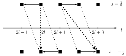
Figure 1: The action of the operator $\mathcal{W}_{1}^{0}$ (thick dotted arrows) on the states $\Psi_{E,2l,+}$ and $\Psi_{E,2l+1,+}$ as a sequential action of $\tilde{Q}_{1}^{0}$ (solid arrows) and $Q_{1}^{0}$ (thin dotted arrows). Black squares represent the eigenstates $\Psi_{E,l,s}$ with corresponding values of $l$ and $s$.

Notice that for the choice (3.8) of the grading operator, each of the four pairs of the odd supercharges (3.10)

$$(Q_{1}^{\gamma},Q_{2}^{\gamma}),\qquad(Q_{3}^{\gamma},Q_{4}^{\gamma}),\qquad(Q_{1}^{\gamma},Q_{3}^{\gamma}),\qquad(Q_{2}^{\gamma},Q_{4}^{\gamma})$$ (3.21)

generates the $N=2$ supersymmetry, see Eq. (3.11). Similarly, the two pairs

$$(Q_{1+}^{\gamma},Q_{1-}^{\gamma}),\qquad(Q_{2+}^{\gamma},Q_{2-}^{\gamma})$$ (3.22)

generate the deformed $N=2$ supersymmetry of the form

$$\{Q_{as}^{\gamma},Q_{as^{\prime}}^{\gamma}\}=2\delta_{ss^{\prime}}\hat{\Pi}_{s}\mathcal{H}_{\alpha}^{\gamma},\qquad a=1,2,\quad s,s^{\prime}=+,-\,.$$ (3.23)

Here $Q_{1\pm}^{\gamma}=\frac{1}{2}(Q_{1}^{\gamma}\pm Q_{4}^{\gamma})=\hat{\Pi}_{\pm}Q_{1}^{\gamma}$, $Q_{2\pm}^{\gamma}=\frac{1}{2}(Q_{2}^{\gamma}\pm Q_{3}^{\gamma})=\hat{\Pi}_{\pm}Q_{2}^{\gamma}$, and $\hat{\Pi}_{\pm}=\frac{1}{2}(1\pm\sigma_{3}R)$ are the projector operators. Analogously, as we noted above, the integrals (3.15) generate the nonlinear [deformed for the pairs $\mathcal{W}_{a\pm}^{\gamma}$, $a=1,2$, constructed similarly to $Q_{a\pm}^{\gamma}$] $N=2$ supersymmetry. In this case, the projector operators $\hat{\Pi}_{\pm}$ are changed for the projectors $\Pi_{\pm}=\frac{1}{2}(1\pm R)$.

A similar picture is valid for the corresponding fermionic supercharges when we choose $\Gamma=R$ or $\Gamma=\sigma_{3}R$.

In summary of this Section, the spin$-1/2$ Aharonov-Bohm system possesses $N=2$ supersymmetry in two cases only, represented by $\mathcal{H}^{0}_{\alpha}$ and $\mathcal{H}_{\alpha}^{\pi}$. It comes hand-in-hand with the hidden supersymmetry represented by the supercharges (3.1). Both, the standard and the hidden supersymmetries, are unified in the framework of the tri-supersymmetry.

This structure will reveal itself later on in the existence of the three different types of the super-extended anyon systems.

4 Tri-supersymmetry and superconformal symmetry

Besides the usual symmetries, the system possesses dynamical symmetries as well. The Hamiltonian $\mathcal{H}_{\alpha}^{\gamma}$ together with the generators of special conformal transformations (expansions) , $K$, and dilatations, $D$,

$$K=\vec{X}{}^{2}\,,\qquad D=-\frac{1}{2}\left(\vec{X}\vec{\cal{P}}+\vec{\cal{P}}\vec{X}\right)\,,\quad\mbox{where}\quad X_{j}=x_{j}-2t{\cal P}_{j},\quad j=1,2\,,$$ (4.1)

form the $so(2,1)$ Lie algebra

$$[D,K]=2iK\,,\qquad[\mathcal{H}_{\alpha}^{\gamma},K]=4iD\,,\qquad[\mathcal{H}_{\alpha}^{\gamma},D]=2i\mathcal{H}_{\alpha}^{\gamma}\,.$$ (4.2)

The operators (4.1) satisfy the relation $\frac{d}{dt}\mathcal{O}=\partial_{t}\mathcal{O}-i[\mathcal{H}_{\alpha}^{\gamma},\mathcal{O}]=0$ ($\mathcal{O}$ being either $K$ or $D$), that justifies to call them dynamical symmetries. Let us note that the Lie algebra $so(2,1)$ of dynamical symmetries in the context of (spinless) Aharonov-Bohm system was first observed in [27].

As long as $\gamma=0$ or $\pi$, neither $K$ nor $D$ alter the asymptotic behavior of the wave functions prescribed by (2.7). Hence, both operators preserve the domain of $\mathcal{H}^{\gamma}_{\alpha}$. In particular, invariance of the domain of $\mathcal{H}_{\alpha}^{\gamma}$ under the action of $D$ is associated with the scale invariance of the system. The relations (4.2) establish then the conformal symmetry of the model.

Now, we discuss how the dynamical symmetries (4.2) can be incorporated into the framework of the tri-supersymmetry. The operators $K$ and $D$ are even with respect to any of the possible grading operators (3.7). First, we consider the case $\Gamma=\sigma_{3}$, and discuss the structure of the superalgebra that includes $K$ and $D$.

The odd supercharges of tri-supersymmetry are indentified with (3.10) and (3.15), see the table. Let us focus on (3.10). It is well known [16], [17] that the usual $N=2$ supersymmetry associated with the supercharges $Q_{1}^{\gamma}$ and $Q_{2}^{\gamma}$ can be expanded into the superalgebra $osp(2|2)$. The same, up to the deformations, algebraic structure can be obtained when we expand by $K$ and $D$ the $N=2$ supersymmetry associated with any other pair of the supercharges from (3.21), (3.22). The (anti-)commutation relations of the (deformed) superconformal algebra give rise to the additional dynamical symmetries,

$$[Q_{\underline{A}}^{\gamma},K]=-2iS_{\underline{A}}^{\gamma}\,,\quad{\rm where}\quad S_{1}^{\gamma}=X_{1}\sigma_{1}+X_{2}\sigma_{2}\,,$$ (4.3)

and $S_{2}^{\gamma}$, $S_{3}^{\gamma}$ and $S_{3}^{\gamma}$ are related to $S_{1}^{\gamma}$ similarly to (3.10). The $S_{\underline{A}}^{\gamma}$ satisfy the anti-commutation relations

$$\{S_{\underline{A}}^{\gamma},S_{\underline{A}}^{\gamma}\}=2K\,,\quad\underline{A}=1,2,3,4,\qquad\{S_{1}^{\gamma},S_{4}^{\gamma}\}=\{S_{2}^{\gamma},S_{3}^{\gamma}\}=2\sigma_{3}RK\,.$$ (4.4)

For the four odd integrals $Q_{\underline{A}}^{\gamma}$ and $S_{\underline{A}}^{\gamma}$ with $\underline{A}=a=1,2$, we have the nontrivial anti-commutation relations in addition to those presented above,

$$\{S_{a}^{\gamma},Q_{b}^{\gamma}\}=-2\delta_{ab}D+2\epsilon_{ab}{\cal J}\,,$$ (4.5)

$$[\mathcal{H}_{\alpha}^{\gamma},S_{a}^{\gamma}]=-2iQ_{a}^{\gamma}\,,\quad[K,Q_{a}^{\gamma}]=2iS_{a}^{\gamma}\,,\quad[D,Q_{a}^{\gamma}]=-iQ_{a}^{\gamma}\,,\quad[D,S_{a}^{\gamma}]=iS_{a}^{\gamma}\,,$$ (4.6)

$$[{\cal J},Q_{a}^{\gamma}]=-i\epsilon_{ab}Q_{b}^{\gamma}\,,\qquad[{\cal J},S_{a}^{\gamma}]=-i\epsilon_{ab}S_{b}^{\gamma}\,,$$ (4.7)

where ${\cal J}=J+\sigma_{3}$, which correspond to the $osp(2|2)$ superalgebra.

In the case of the odd generators $Q_{\underline{A}}^{\gamma}$ and $S_{\underline{A}}^{\gamma}$ with $\underline{A}=3,4$ we have the same $osp(2|2)$ superalgebra with the change of the indices $1\rightarrow 4$, $2\rightarrow 3$ in correspondence with relations $Q_{\underline{4}}^{\gamma}=\sigma_{3}RQ_{\underline{1}}^{\gamma}$, $Q_{\underline{3}}^{\gamma}=\sigma_{3}RQ_{\underline{2}}^{\gamma}$, and the same relations for the integrals $S^{\gamma}$.

The other two pairs of $Q_{\underline{A}}^{\gamma}$ from (3.21), and the two pairs in (3.22) can be extended in the similar vain, giving rise to corresponding pairs of $S_{\underline{A}}^{\gamma}$, and the pairs $(S_{a+}^{\gamma}$, $S^{\gamma}_{a-}$), $a=1,2$, respectively. The resulting algebras are of the same form as (4.5)–(4.7), but with some of the (anti)-commutation relations to be deformed by inclusion of the factor $\sigma_{3}R$, or the projector as in Eq. (3.23). For instance, $\{S_{1}^{\gamma},Q_{3}^{\gamma}\}=2\sigma_{3}R\,{\cal J}$, cf. (4.5). Hence, we get six different (deformed) representations of the superalgebra $osp(2|2)$ that are included in the finite-dimensional extension of the superalgebra $osp(2|2)$ generated by $\mathcal{H}^{\gamma}_{\alpha}$, $K$, $D$ and the supercharges $Q^{\gamma}_{\underline{A}}$. Note that the operator $\sigma_{3}R$ commutes with all the generators of the $osp(2|2)$ here.

Similarly to (4.3), the commutators of (3.9) with $K$ generate a new set of dynamical integrals,

$$[\tilde{Q}_{\underline{A}}^{\gamma},K]=-2i\tilde{S}_{\underline{A}}^{\gamma}\,,$$ (4.8)

which are fermionic operators for $\Gamma=\sigma_{3}$. But when we expand here the set of the even, $\mathcal{H}_{\alpha}^{\gamma}$, $K$, $D$, ${\cal J}$, and odd, $Q_{\underline{A}}^{\gamma}$, $S_{\underline{A}}^{\gamma}$, generators with the bosonic operators $\tilde{Q}_{\underline{A}}^{\gamma}$ or/and fermionic operators $\mathcal{W}_{\underline{A}}^{\gamma}$, an infinite number of the new operators appears.

The picture is similar for other choices of the grading operator. For instance, for $\Gamma=R$, the (deformed) finite-dimensional extension of the $osp(2|2)$ superalgebra is obtained if we supply the generators of the conformal symmetry with one (not both) of the two sets of the fermionic operators, $Q_{\underline{A}}^{\gamma}$ or $\tilde{Q}_{\underline{A}}^{\gamma}$. The same is valid for the case $\Gamma=\sigma_{3}R$, when the $so(2,1)$ generators are supplied by the fermionic operators $\tilde{Q}_{\underline{A}}^{\gamma}$. As soon, however, as we supply the $so(2,1)$ generators (4.1) with the integrals $\mathcal{W}_{\underline{A}}^{\gamma}$, we get the infinite superalgebra.

Hence, the extension of the tri-supersymmetry by the dynamical integrals $D$ and $K$ gives rise to the infinite superalgebra for any choice of the grading operator. As we saw, six (deformed) superalgebras $osp(2|2)$ are included as finite subalgebras. Note that the infinite superalgebra still has the central element $\mathcal{Z}^{\gamma}$, see (3.19).

5 Tri-supersymmetry and three types of supersymmetric anyons

We provide now an alternative interpretation of the results presented in the previous Sections, applying them to the theory of anyons. We elaborate the idea for the system described by $\mathcal{H}_{\alpha}^{0}$. The case of $\mathcal{H}_{\alpha}^{\pi}$ can be treated similarly.

The dynamical realization of the anyons [28] that was proposed by Wilczek in [7], is based, in fact, on the Aharonov-Bohm effect. In such a picture, anyon is considered as a “composite”, statistically charged particle that is either boson or fermion, to which a magnetic vortex is attached. The presence of the vortex provides the peculiar statistical properties of the anyons. Consider the system of two identical non-relativistic anyons in such a picture. It is assumed that each particle feels only the potential produced by the vortex attached to the other particle. The Hamiltonian of the system we denote as

$$H_{any}=2\sum_{I=1}^{2}\left(\vec{p}_{I}-\vec{a}_{I}(\vec{r})\right)^{2}\,,$$ (5.1)

see [8]. Index $I\,$ labels the individual particles (whose masses are $m_{1}=m_{2}=4$) with the momenta $\vec{p}_{I}=-i\partial/\partial\vec{x}_{I}$. The vector $\vec{r}\,$ is a relative coordinate of the particles, $\vec{r}=\vec{x}_{1}-\vec{x}_{2}$. The potentials $\vec{a}_{I}$,

$$a_{1}^{k}(\vec{r})=-a_{2}^{k}(\vec{r})=\frac{1}{2}\alpha\epsilon^{kl}\frac{r^{l}}{\vec{r}\,{}{}^{2}}\,,$$ (5.2)

encode the “statistical” interaction of the particles. When we write the Hamiltonian in the center-of-the-mass coordinates, the relative motion of the particles is governed by the effective Hamiltonian

$$H_{rel}=-\partial_{r}^{2}-\frac{1}{r}\partial_{r}+\frac{1}{r^{2}}(-i\partial_{\varphi}+\alpha)^{2}\,,$$ (5.3)

where $r$ and $\varphi$ are the polar coordinates of the $\vec{r}$.

Formally, this operator coincides with the spinless Hamiltonians $H_{\alpha}^{0}$ and $H_{\alpha}^{AB}$ of (2.9). But its domain is quite different. The domain of (5.3) reflects the nature of the anyons and is composed of functions which are either symmetric or anti-symmetric under the change $\varphi\rightarrow\varphi+\pi$. The periodicity of wave functions depends, in turn, on the nature of the interacting particles. The two-body wave function has to be symmetric in $\pi$ (invariant with respect to the exchange of the particles) as long as we deal with anyons based on bosons. When the vortices are attached to fermions, the wave function has to change its sign after the substitution $\varphi\rightarrow\varphi+\pi$. Hence, we have

$$\psi_{\alpha}(r,\varphi)=\sum_{l}e^{il\varphi}f_{\alpha,l}(r),\quad l\in\left\{\begin{array}[]{l}2\mathbb{Z}\ \mbox{for anyons based on bosons\,,}\\ 2\mathbb{Z}+1\ \mbox{for anyons based on fermions\,.}\end{array}\right.$$ (5.4)

Notice that the system can be described alternatively by the free Hamiltonian $H_{rel}=-\partial_{r}^{2}-1/r\partial_{r}+(-i\partial_{\varphi})^{2}/r^{2}$. However, the wave functions have to acquire the gauge factor $e^{i\alpha\varphi}$ in this case to keep the description equivalent to (5.3) and (5.4), i.e. $\psi_{\alpha}(r,\varphi)=e^{i\varphi\alpha}\sum_{l}e^{il\varphi}f_{\alpha,l}(r)$. In this alternative picture, after the substitution $\varphi\rightarrow\varphi+\pi$ the wave functions acquire the phase $e^{i\pi\alpha}$ which interpolates between the values corresponding to Bose and Fermi statistics. We prefer to use the framework (5.4), where the wave functions are $2\pi$-periodic for any value of $\alpha$.

Let us return to our current system. Instead to treat its Hamiltonian as that of Pauli, we consider it as a direct sum of four operators, just as the $4\times 4$ matrix operator

$$\mathcal{H}^{\gamma=0}_{\alpha}=diag\,(H^{0}_{\alpha,+},H^{0}_{\alpha,-},H^{AB}_{\alpha,+},H^{AB}_{\alpha,-})\,,\qquad H^{0}_{\alpha,\pm}=H^{0}_{\alpha}\Pi_{\pm},\quad H^{AB}_{\alpha,\pm}=H^{AB}_{\alpha}\Pi_{\pm}\,,$$ (5.5)

where we used the projectors $\Pi_{\pm}=\frac{1}{2}(1\pm R)$ which separate symmetric and anti-symmetric under displacement of $\varphi$ in $\pi$ wave functions. We remind that the nonzero elements of this diagonal Hamiltonian operator coincide as differential operators but can differ in their domains. The singular wave functions are contained in the domain of $H^{0}_{\alpha,-}$ only. The operator $H^{AB}_{\alpha,-}$ acts on regular functions which are anti-periodic in $\pi$. The operators $H^{0}_{\alpha,+}$ and $H^{AB}_{\alpha,+}$ coincide actually in their domains and describe the same physical setting.

Now, each of the operators $H^{AB}_{\alpha,\pm}$ and $H^{0}_{\alpha,\pm}$ can be interpreted as the Hamiltonian of the relative motion of the two identical anyons. Indeed, they coincide formally with (5.3) and their domains are composed of either odd or even partial waves (5.4). The regularity of the wave functions of $H_{\alpha,\pm}^{AB}$ and $H_{\alpha,+}^{0}$ can be understood as a manifestation of the hard core interaction of the anyons. The singular behavior at $r\sim 0$ in the domain of $H_{\alpha,-}^{0}$ can be reinterpreted as the nontrivial contact interaction of the particles [29]. Notice that this interaction appears for one partial wave only, all other partial waves are regular at the origin.

We conclude, therefore, that $H^{AB}_{\alpha,+}$ and $H^{0}_{\alpha,+}$ describe two anyons based on bosons. Similarly, $H_{\alpha,-}^{AB}$ and $H^{0}_{\alpha,-}$ describe the systems of two anyons based on fermions.

We identify now the sense of the cornerstones of the tri-supersymmetry, the integrals of motion $Q_{1}^{0}$, $\tilde{Q}_{1}^{0}$ and $\mathcal{W}_{1}^{0}$, in this framework. Keeping in mind (2.2) and (3.1) and the splitting of $\mathcal{D}(\mathcal{H}_{\alpha}^{0})$ which was made implicitly in (5.5), we can write

$$Q_{1}^{0}=\left(\begin{array}[]{cccc}0&0&0&q_{+}\\ 0&0&q_{+}&0\\ 0&q_{-}&0&0\\ q_{-}&0&0&0\end{array}\right),\,\,\tilde{Q}_{1}^{0}=\left(\begin{array}[]{cccc}0&q_{-}&0&0\\ q_{+}&0&0&0\\ 0&0&0&q_{+}\\ 0&0&q_{-}&0\end{array}\right),\,\,\mathcal{W}_{1}^{0}=\left(\begin{array}[]{cccc}0&0&q_{+}q_{-}&0\\ 0&0&0&q_{+}^{2}\\ q_{-}q_{+}&0&0&0\\ 0&q_{-}^{2}&0&0\end{array}\right),$$ (5.6)

where $q_{\pm}$ are defined in (2.2). The nontrivial matrix elements of the commutation relation $[Q_{1}^{0},\mathcal{H}^{0}_{\alpha}]=0$ give

$$H_{\pm}^{0}q_{+}=q_{+}H_{\mp}^{AB}\,,\qquad H_{\pm}^{AB}q_{-}=q_{-}H_{\mp}^{0}\,,$$ (5.7)

where $H_{\pm}^{0}=H_{\alpha,\pm}^{0}$, $H_{\pm}^{AB}=H_{\alpha,\pm}^{AB}$. The commutator $[\tilde{Q}_{1}^{0},\mathcal{H}^{0}_{\alpha}]=0$ gives rise to the operator equations

$$H_{\pm}^{0}q_{\mp}=q_{\mp}H_{\mp}^{0}\,,\qquad H_{\pm}^{AB}q_{\pm}=q_{\pm}H_{\mp}^{AB}\,,$$ (5.8)

and the commutator $[\mathcal{W}_{1}^{0},\mathcal{H}_{\alpha}^{0}]=0$ can be rewritten as

$$H_{-}^{AB}q_{-}^{2}=q_{-}^{2}H_{-}^{0},\qquad H_{-}^{0}q_{+}^{2}=q_{+}^{2}H_{-}^{AB},\quad H_{+}^{AB}q_{-}q_{+}=q_{-}q_{+}H_{+}^{0},\quad H_{+}^{0}q_{+}q_{-}=q_{+}q_{-}H_{+}^{AB}.$$ (5.9)

Due to the identity $H_{\alpha,+}^{0}=H_{\alpha,+}^{AB}$, the last two relations tell that $q_{+}q_{-}=q_{-}q_{+}$ is a symmetry of $H_{\alpha,+}^{AB}$ (as well as of $H_{\alpha,+}^{0}$). However, it is trivial since $q_{+}q_{-}$ coincides with the Hamiltonian. Not all the relations in (5.7)–(5.9) are independent. We reduce their number using the identity $H_{\alpha,+}^{0}=H_{\alpha,+}^{AB}$. The independent relations are

$$H_{+}^{0}q_{-}=q_{-}H_{-}^{0}\,,\qquad q_{+}H_{+}^{0}=H_{-}^{0}q_{+}\,,$$ (5.10)

$$H_{+}^{0}q_{+}=q_{+}H_{-}^{AB}\,,\qquad q_{-}H_{+}^{0}=H_{-}^{AB}q_{-}\,,$$ (5.11)

$$H_{-}^{AB}q_{-}^{2}=q_{-}^{2}H_{-}^{0}\,,\qquad q_{+}^{2}H_{-}^{AB}=H_{-}^{0}q_{-}^{2}\,.$$ (5.12)

Each of the relations (5.10), (5.11) can be understood as intertwining relation of the $N=2$ standard supersymmetry [3]. The relations (5.12) give rise to the nonlinear (the second order) supersymmetry [24]. We have, therefore, three supersymmetric systems, for which the superpartner Hamiltonians are two-particle anyon systems.

The relations (5.10) and (5.11) give rise to the linear $N=2$ supersymmetry

$$\left[\mathbf{q}^{(j)}_{a},\mathbf{h}^{(j)}\right]=0,\quad\left\{\mathbf{q}^{(j)}_{a},\mathbf{q}^{(j)}_{b}\right\}=2\delta_{a,b}\mathbf{h}^{(j)}\,,\quad j,a,b=1,2\,,$$ (5.13)

represented, in case of (5.10), by the matrix Hamiltonians and corresponding supercharge operators

$$\mathbf{h}^{(1)}=\left(\begin{array}[]{cc}H_{+}^{0}&0\\ 0&H_{-}^{0}\end{array}\right),\quad\mathbf{q}^{(1)}_{1}=\left(\begin{array}[]{cc}0&q_{-}\\ q_{+}&0\end{array}\right),\quad\mathbf{q}^{(1)}_{2}=i\left(\begin{array}[]{cc}0&-q_{-}\\ q_{+}&0\end{array}\right),$$ (5.14)

while in the case of (5.11) by the operators

$$\mathbf{h}^{(2)}=\left(\begin{array}[]{cc}H_{+}^{0}&0\\ 0&H_{-}^{AB}\end{array}\right),\quad\mathbf{q}^{(2)}_{1}=\left(\begin{array}[]{cc}0&q_{+}\\ q_{-}&0\end{array}\right),\quad\mathbf{q}^{(2)}_{2}=i\left(\begin{array}[]{cc}0&-q_{+}\\ q_{-}&0\end{array}\right).$$ (5.15)

The supercharges change the nature of the anyons in the two-body systems; they transform the boson-based anyons of $H_{+}^{0}$ into the fermion-based anyons of either $H_{-}^{0}$ or $H_{-}^{AB}$. In addition, they change the contact interaction in $\mathbf{h}^{(1)}$ from the hard-core interaction of $H_{+}^{0}$ to the nontrivial contact interaction of $H_{-}^{0}$ (and vice versa).

The situation differs in the system associated with (5.12). The $N=2$ supersymmetry generated by the operators

$$\mathbf{h}^{(3)}=\left(\begin{array}[]{cc}H_{-}^{0}&0\\ 0&H_{-}^{AB}\end{array}\right),\quad\mathbf{q}^{(3)}_{2}=\left(\begin{array}[]{cc}0&q_{+}^{2}\\ q_{-}^{2}&0\end{array}\right),\quad\mathbf{q}^{(3)}_{2}=i\left(\begin{array}[]{cc}0&-q_{+}^{2}\\ q_{-}^{2}&0\end{array}\right)$$ (5.16)

is nonlinear,

$$\left[\mathbf{q}^{(3)}_{a},\mathbf{h}^{(3)}\right]=0,\quad\left\{\mathbf{q}^{(3)}_{a},\mathbf{q}^{(3)}_{b}\right\}=2\delta_{ab}\left(\mathbf{h}^{(3)}\right)^{2}\,,\quad a,b=1,2\,.$$ (5.17)

The supercharges preserve the nature of the anyons and just alter the contact interaction of the two-body systems described by $H_{-}^{0}$ and $H_{-}^{AB}$.

The role of the grading operator in all the three cases (5.14)–(5.16) is played by $\sigma_{3}$.

Concluding, coherently with the tri-supersymmetric structure of the system $\mathcal{H}^{0}_{\alpha}$ described in the previous Sections, the integrals $Q_{1}^{0}$, $\tilde{Q}_{1}^{0}$ and $\mathcal{W}_{1}^{0}$ give rise to the three different supersymmetric models (5.14)–(5.16) of the two-body systems of interacting anyons. The first two models [each is composed from the boson- and fermion-based anyons] are described by a linear $N=2$ supersymmetric structure. The third one, (5.16), composed from the two fermion-based anyon subsystems, is described by the nonlinear, second order $N=2$ supersymmetry. Due to the results of Section 4, the systems (5.14) and (5.15) have the superconformal symmetry generated, besides the supercharges and the Hamiltonian, by the diagonal (even) operators $K$ and $D$, and by the odd dynamical symmetries $\mathbf{s}_{1}^{(j)}=i[\mathbf{q}^{(j)}_{1},K]$, $\mathbf{s}_{2}^{(j)}=i\sigma_{3}\mathbf{s}_{1}^{(j)}$. In contrary, although the supersymmetric Hamiltonian $\mathbf{h}^{(3)}$ has the conformal symmetry, its supercharges cannot be included in the closed, finite Lie superalgebra together with the dynamical symmetries $K$ and $D$. As we saw in the Section 4, the superalgebra would be infinitely generated in this case.

The similar treatment applies to the system described by $\mathcal{H}^{\pi}_{\alpha}$. In that case, the subsystems $H_{-}^{AB}$ and $H_{-}^{\pi}$ would coincide.

6 Discussion and outlook

The system of the spin-1/2 particle in the field of the magnetic vortex, that is described by the Hamiltonians $\mathcal{H}_{\alpha}^{0}$ or $\mathcal{H}_{\alpha}^{\pi}$, has a rich algebraic supersymmetry structure. We found that the existence of the standard $N=2$ supersymmetry is accompanied by the nonlocal supercharges (3.1) of the hidden supersymmetry. They form a different realization of the $N=2$ supersymmetry of the model. Both the local and nonlocal supercharges can be unified in the framework of the tri-supersymmetry. There are three possible candidates for the grading operator, see (3.7), and three sets (3.9), (3.10) and (3.15) of the operators which permute in the role of the fermionic supercharges, dependently on the choice of the grading operator.

The tri-supersymmetry can be extended by the conformal symmetry (4.2) of the model. The extension gives rise to the infinitely generated superalgebra. It contains, however, the (deformed) finite dimensional extension of the superconformal symmetry $osp(2|2)$.

We have applied the obtained results to the theory of anyons, by reinterpreting the system and its algebraic structure in terms of the supersymmetric two-body model of the interacting anyons (5.14)–(5.16). Coherently with the described tri-supersymmetric structure, the three different associated anyon systems are characterized by either linear, or non-linear $N=2$ supersymmetry graded by $\sigma_{3}$.

The setting with integer magnetic flux, which is unitary equivalent to a free particle case with $\alpha=0$, is worth a separate note and a related comment on translational invariance. As we observed, for $\alpha=0$ the system is specified uniquely, and its wave functions (2.5) and (2.6) are regular at the origin. It has the standard $N=2$ supersymmetry given by the supercharges $Q_{1}$ and $Q_{2}$. The supercharges of the hidden supersymmetry can be defined as well. The simplicity of the $\alpha=0$ case, however, admits a greater freedom in their definition; all the operators of the two-parameter family

$$\tilde{Q}_{1,\epsilon_{1},\epsilon_{2}}=diag(\mathcal{P}_{1}+\epsilon_{1}iR\mathcal{P}_{2},\mathcal{P}_{1}+\epsilon_{2}iR\mathcal{P}_{2}),\quad\tilde{Q}_{2,\epsilon_{1},\epsilon_{2}}=iR\tilde{Q}_{1,\epsilon_{1},\epsilon_{2}},\quad\alpha=0,$$ (6.1)

are well defined for $\epsilon_{1},\epsilon_{2}=\pm 1$. The set of integrals (6.1) is equivalent to the set

$$diag(\mathcal{P}_{j},0),\quad diag(iR\mathcal{P}_{j},0),\quad diag(0,\mathcal{P}_{j}),\quad diag(0,iR\mathcal{P}_{j}),\quad j=1,2,$$ (6.2)

that just manifests the translational invariance and the reflection (rotation in $\pi$) symmetry of the spin-up and spin-down components of the free-particle Hamiltonian. When the magnetic flux is switched on, the translational invariance of the system breaks down. Indeed, the generators $\mathcal{P}_{1}$ and $\mathcal{P}_{2}$ are not physical as they alter the boundary condition (2.7), and consequently their commutator with $\mathcal{H}_{\alpha}^{\gamma}$ is not well defined. The breakdown of translational invariance reduces the set of symmetries (6.1) in half, leaving just the operators which coincide with (3.1). In this sense, the supercharges of the hidden supersymmetry $\tilde{Q}_{1}^{\gamma}$ and $\tilde{Q}_{2}^{\gamma}$ can be understood as the successors of the translational symmetry. A deeper investigation of this point in the context of the associated Galilei symmetry goes, however, beyond the scope of the present paper and will be presented elsewhere.

In conclusion, it would be interesting to apply the approach presented here to investigation of supersymmetry in the system of the spin-1/2 particle in the field of the magnetic monopole, where the issue of the domain of definition is also essential [30], as well as in the setting with several magnetic fluxes embedded into the homogeneous magnetic field [31], and to test them on the presence of the hidden supersymmetry.

Acknowledgements. The work has been partially supported by DICYT (USACH), MECESUP Project FSM0605, and FONDECYT Grants 1095027, 3100123 and 3085013, Chile, by CONICET (PIP 01787), UNLP (Proy. 11/X492) and ANPCyT (PICT-2007-00909), Argentina, by the grant LC06002 of the Ministry of Education, Youth and Sports of the Czech Republic, and by Spanish Ministerio de Educación under Project SAB2009-0181 (sabbatical grant of MSP). H.F. is indebted to the Physics Department of Santiago University (Chile) for hospitality. The Centro de Estudios Científicos (CECS) is funded by the Chilean Government through the Millennium Science Initiative and the Centers of Excellence Base Financing Program of Conicyt. CECS is also supported by a group of private companies which at present includes Antofagasta Minerals, Arauco, Empresas CMPC, Indura, Naviera Ultragas and Telefónica del Sur.

References

• [1] Y. Aharonov and A. Casher, “The ground state of a spin 1/2 charged particle in a two-dimensional magnetic field,” Phys. Rev.  A 19 (1979) 2461.
• [2] L. E. Gendenshtein and I. V. Krive, “Supersymmetry in quantum mechanics,” Sov. Phys. Usp.  28 (1985) 645 [Usp. Fiz. Nauk 146 (1985) 553].
• [3] F. Cooper, A. Khare and U. Sukhatme, “Supersymmetry and quantum mechanics,” Phys. Rept.  251 (1995) 267 [arXiv:hep-th/9405029].
• [4] L. D. Landau and E. M. Lifshitz, Course of Theoretical Physics, Vol. 3. Quantum Mechanics. Non-Relativistic Theory, p. 458 (3ed., Pergamon, 1991); A. Galindo and P. Pascual, Quantum Mechanics, Vol. 2, p. 215 (Springer-Verlag, Berlin, 1990).
• [5] R. B. Laughlin, “Quantized Hall conductivity in two-dimensions,” Phys. Rev.  B 23 (1981) 5632.
• [6] Y. Aharonov and D. Bohm, “Significance of electromagnetic potentials in the quantum theory,” Phys. Rev.  115 (1959) 485.
• [7] F. Wilczek, “Magnetic flux, angular momentum, and statistics,” Phys. Rev. Lett.  48 (1982) 1144; “Quantum mechanics of fractional spin particles,” Phys. Rev. Lett.  49 (1982) 957.
• [8] F. Wilczek, “Fractional statistics and anyon superconductivity,” World Scientific, Singapore (1990), A. Khare, “Fractional statistics and quantum theory,” World Scientific, Singapore (1997).
• [9] A. Vilenkin, “Cosmic strings and domain walls,” Phys. Rept.  121 (1985) 263; M. G. Alford and F. Wilczek, “Aharonov-Bohm interaction of cosmic strings with matter,” Phys. Rev. Lett.  62 (1989) 1071; C. Filgueiras and F. Moraes, “The bound state Aharonov-Bohm effect around a cosmic string revisited,” Phys. Lett.  A 361 (2007) 13 [arXiv:gr-qc/0509100].
• [10] P. de Sousa Gerbert, “Fermions in an Aharonov-Bohm field and cosmic strings,” Phys. Rev.  D 40 (1989) 1346.
• [11] A. Bachtold et al, “Aharonov-Bohm oscillations in carbon nanotubes,” Nature 397 (1999) 673; S. Zaric et al, “Optical signatures of the Aharonov-Bohm phase in single-walled carbon nanotubes,” Science 304 (2004) 1129; H. Ajiki and T. Ando, “Aharonov-Bohm effect in carbon nanotubes,” Physica B 201 (1994) 349; W. Tian and S. Datta, “Aharonov-Bohm-type effect in graphene tubules: A Landauer approach,” Phys. Rev. B 49 (1994) 5097; R. Jackiw, A. I. Milstein, S. Y. Pi and I. S. Terekhov, “Induced current and Aharonov-Bohm effect in graphene,” Phys. Rev. B 80 (2009) 033413 [arXiv:0904.2046 [cond-mat.mes-hall]].
• [12] S. Albeverio, F. Gesztesy, R. Høegh-Krohn, and H. Holden, “Solvable models in quantum mechanics”, Springe-Verlag, New York (1988).
• [13] V. A.  Geyler, P. Šťovíček, “On the Pauli operator for the Aharonov-Bohm effect with two solenoids”, J. Math. Phys. 45, (2004) 51; L. Da̧browski and P. Šťovíček, “Aharonov-Bohm effect with delta type interaction,” J. Math. Phys.  39 (1998) 47.
• [14] C. R. Hagen, “Aharonov-Bohm scattering of particles with spin,” Phys. Rev. Lett.  64 (1990) 503; F.A.B. Coutinho, Y. Nogami, J. Fernando Perez, “Self-adjoint extensions of the Hamiltonian for a charged particle in the presence of a thread of magnetic flux,” Phys. Rev.  A 46 (1992) 6052; F. A. B. Coutinho and J. Fernando Perez, “Boundary conditions in the Aharonov-Bohm scattering of Dirac particles and the effect of Coulomb interaction,” Phys. Rev. D 48 (1993) 932; F. A. B. Coutinho, Y. Nogami, J. Fernando Perez and F. M. Toyama, “Self-adjoint extensions of the Hamiltonian for a charged spin- 1/2 particle in the Aharonov-Bohm field,” J. Phys. A 27 (1994) 6539; A. Moroz, “The single-particle density of states, bound states, phase-shift flip, and a resonance in the presence of an Aharonov-Bohm potential,” Phys. Rev.  A 53 (1996) 669 [arXiv:cond-mat/9504107].
• [15] A. O. Barut and P. Roy, “Dynamical groups and supersymmetry. 2. Supersymmetric Aharonov-Bohm and anyon systems,” Mod. Phys. Lett.  A 8, 3507 (1993).
• [16] C. J. Park, “The dynamical supersymmetry of the point magnetic vortex”, Nucl. Phys. B 376 (1992) 99.
• [17] C. Duval and P. A. Horvathy, “On Schrodinger superalgebras,” J. Math. Phys.  35 (1994) 2516 [arXiv:hep-th/0508079]; P. A. Horvathy, “Dynamical (super)symmetries of monopoles and vortices,” Rev. Math. Phys.  18 (2006) 329 [arXiv:hep-th/0512233]; P. A. Horvathy and P. Zhang, “Vortices in (abelian) Chern-Simons gauge theory,” Phys. Rept.  481 (2009) 83 [arXiv:0811.2094 [hep-th]].
• [18] F. Correa, V. Jakubský, L. M. Nieto and M. S. Plyushchay, “Self-isospectrality, special supersymmetry, and their effect on the band structure,” Phys. Rev. Lett.  101 (2008) 030403 [arXiv:0801.1671 [hep-th]]; F. Correa, V. Jakubský and M. S. Plyushchay, “Finite-gap systems, tri-supersymmetry and self-isospectrality,” J. Phys. A 41 (2008) 485303 [arXiv:0806.1614 [hep-th]].
• [19] F. Correa, V. Jakubský and M. S. Plyushchay, “Aharonov-Bohm effect on AdS2 and nonlinear supersymmetry of reflectionless Poschl-Teller system,” Annals Phys.  324 (2009) 1078 [arXiv:0809.2854 [hep-th]].
• [20] M. Reed, B. Simon, Methods of Modern Mathematical Physics II. Fourier Analysis, Self-Adjointness, Academic Press, New York (1978).
• [21] F. Correa, H. Falomir, V. Jakubský and M. S. Plyushchay, “Hidden superconformal symmetry of spinless Aharonov-Bohm system,” J. Phys. A 43 (2010) 075202 [arXiv:0906.4055 [hep-th]].
• [22] M. S. Plyushchay, “Deformed Heisenberg algebra, fractional spin fields and supersymmetry without fermions,” Annals Phys.  245 (1996) 339 [arXiv:hep-th/9601116]; F. Correa and M. S. Plyushchay, “Hidden supersymmetry in quantum bosonic systems,” Annals Phys.  322 (2007) 2493 [arXiv:hep-th/0605104].
• [23] M. Plyushchay, “Hidden nonlinear supersymmetries in pure parabosonic systems,” Int. J. Mod. Phys.  A 15 (2000) 3679 [arXiv:hep-th/9903130].
• [24] A. A. Andrianov, M. V. Ioffe and V. P. Spiridonov, “Higher derivative supersymmetry and the Witten index,” Phys. Lett.  A 174 (1993) 273 [arXiv:hep-th/9303005]; V.G.Bagrov, and B.F. Samsonov, “Darboux transformation, factorization, and supersymmetry in one-dimensional quantum mechanics,” Theor. Math. Phys. 104 (1995) 1051; D. J. Fernandez C, “SUSUSY quantum mechanics,” Int. J. Mod. Phys.  A 12 (1997) 171 [arXiv:quant-ph/9609009]; S. M. Klishevich and M. S. Plyushchay, “Nonlinear supersymmetry, quantum anomaly and quasi-exactly solvable systems,” Nucl. Phys.  B 606 (2001) 583 [arXiv:hep-th/0012023]; A. A. Andrianov and A. V. Sokolov, “Nonlinear supersymmetry in quantum mechanics: algebraic properties and differential representation,” Nucl. Phys.  B 660 (2003) 25 [arXiv:hep-th/0301062]; A. A. Andrianov and F. Cannata, “Nonlinear supersymmetry for spectral design in quantum mechanics,” J. Phys. A 37 (2004) 10297 [arXiv:hep-th/0407077].
• [25] A. Galindo and P. Pascual, Quantum Mechanics, Vol. 1, p. 250 (Springer-Verlag, Berlin, 1990).
• [26] F. Correa, L. M. Nieto and M. S. Plyushchay, “Hidden nonlinear $su(2|2)$ superunitary symmetry of N=2 superextended 1D Dirac delta potential problem,” Phys. Lett.  B 659 (2008) 746 [arXiv:0707.1393 [hep-th]];
• [27] R. Jackiw, “Dynamical symmetry of the magnetic vortex,” Annals Phys.  201 (1990) 83.
• [28] J. M. Leinaas and J. Myrheim, “On the theory of identical particles,” Nuovo Cim.  B 37 (1977) 1.
• [29] C. Manuel and R. Tarrach, “Do anyons contact interact?,” Phys. Lett.  B 268 (1991) 222.
• [30] E. D’Hoker and L. Vinet, “Supersymmetry of the Pauli equation in the presence of a magnetic monopole,” Phys. Lett.  B 137 (1984) 72; E. Karat and M. B. Schulz, “Selfadjoint extensions of the Pauli equation in the presence of a magnetic monopole,” Annals Phys.  254 (1997) 11.
• [31] T. Mine, “The Aharonov-Bohm solenoids in a constant magnetic fields,” Ann. Henri Poincaré 6 (2005) 125; T. Mine, Y. Nomura,“ Periodic Aharonov-Bohm solenoids in a constant magnetic field”, Rev. Math. Phys. 18 (2006) 913.