Abstract

The continuous-variable coherent (conat) channel is a useful resource for coherent communication, producing coherent teleportation and coherent superdense coding. We extend the conat channel to multiparty conditions by proposing definitions about multiparty position-quadrature conat channel and multiparty momentum-quadrature conat channel. We additionally provide two methods to implement this channel using linear optics. One method is the multiparty version of coherent communication assisted by entanglement and classical communication (CCAECC). The other is multiparty coherent superdense coding.

OCIS codes: (060.5565) Quantum communications; (270.5565) Quantum communications.

1 Introduction

The coherent bit (cobit) with discrete variables (DV) proposed by Aram Harrow [2] is a powerful resource intermediate between a quantum bit (qubit) and a classical bit (cbit). In [2], a qubit channel can be described as: $|x\rangle^{A}\rightarrow|x\rangle^{B}$ ($\{|x\rangle\}_{x\in\{0,1\}}$ is a basis for $\mathbb{C}^{2}$. A is sender Alice. B is receiver Bob). A cbit channel is: $|x\rangle^{A}\rightarrow|x\rangle^{B}|x\rangle^{E}$ (E is inaccessible environment).

A bipartite cobit channel with DV can be described by the isometry: $|x\rangle^{A}\rightarrow|x\rangle^{A}|x\rangle^{B}$. For example, if Alice possesses an arbitrary qubit: $|\psi\rangle^{A}=\alpha|0\rangle^{A}+\beta|1\rangle^{A}$ and transmits it through a cobit channel, the channel generates: $|\phi\rangle^{AB}=\alpha|0\rangle^{A}|0\rangle^{B}+\beta|1\rangle^{A}|1\rangle^{B}$. The process maintains the coherent superposition property of Alice’s original state, this is the reason for the channel’s name[2]. In [3], Wilde and Brun compared and pointed out the differences and connections among concepts about classical communication, quantum communication, entanglement and cobit channel.

Recently, Wilde, Krovi, and Brun extended cobit channel with discrete variables to continuous variables (CV), and they introduced the concept of ‘conat channel’[4] as the CV counterpart of the DV ’cobit channel’. In their work, Wilde and Brun proposed definitions of ideal position-quadrature (PQ) and momentum-qudrature (MQ) conat channel in Schroedinger-picture: $|x\rangle^{A}\rightarrow|x\rangle^{A}|x\rangle^{B}$,$|p\rangle^{A}\rightarrow|p\rangle^{A}|p\rangle^{B}$ where $|x\rangle$ and $|p\rangle$ represents position and momentum eigenstate respectively. Nonideal (finitely squeezed) conat channels are also discussed in the Heisenberg picture[10].

The coherent channel provides for coherent communication. Coherent communication has several useful characteristics and applications. It provides a coherent version of continuous-variable teleportation and continuous-variable superdense coding, and they are proved dual under resource reversal [2, 5]. In addition, it can be applied in remote state preparation (RSP), consuming less entanglement than standard ways [2]. Moreover, coherent communication also proves useful in error correcting codes [6, 7].

In this paper, we extend the notion of conat channel to multiparty situations in order to perform multiparty coherent communication. Additionally, we propose two methods of implementation with linear optical techniques and analyze the noise accumulation in different EPR [8] resources. Multiparty conat channel inherits all the useful properties from bipartite conat channel.

Our paper is organized as follows. In Section 2, we provide a general definition of multiparty position-quadrature (PQ) and momentum-qudrature (MQ) conat channel in Heisenberg representation. In Section 3, two implementations of the protocol with linear optical devices are outlined. A brief conclusion is given in Section 4.

2 Definitions of multiparty conat channel

We propose a general definition of multiparty position-quadrature (PQ) and momentum-qudrature (MQ) conat channel in Heisenberg representation[10].

The channel has only one sender: Alice and $n$ receivers: Alice, Bob, Charlie $\cdots$ and Nick. Notice that the sender is also among the receivers. We denote sender Alice as $A$ and the received massage after the channel as $A^{\prime},B^{\prime},C^{\prime},\cdots,N^{\prime}$. The multiparty PQ conat channel $\tilde{\Delta}_{X}$ copies the position quadrature of the sender to all the receivers with respective noise. The resulting multimode state is similar to multiparty Greenberger-Horne-Zeilinger (GHZ) entangled states[9]. The difference is that the total momentum of the output modes is close to the original momentum of the sender $\hat{p}_{A}$, encoding the transmitted message into all the receivers involved in this channel, while the total momentum of GHZ entangled state is zero. Multiparty MQ conat channel is similarly defined.

Definition 1: A multiparty PQ conat channel $\tilde{\Delta}_{X}$.

Mapping:

$$[\hat{x}_{A}\ \hat{p}_{A}]^{T}\rightarrow[\hat{x}_{A^{\prime}}\ \hat{p}_{A^{\prime}}\ \hat{x}_{B^{\prime}}\ \hat{p}_{B^{\prime}}\ \cdots\ \hat{x}_{N^{\prime}}\ \hat{p}_{N^{\prime}}]^{T}$$ (1)

Constraints:

$$\begin{cases}{\hat{x}_{A^{\prime}}}=\hat{x}_{A}\\ \hat{x}_{B^{\prime}}=\hat{x}_{A}+\hat{x}^{\ 1}_{\Delta_{X}}\\ \hat{x}_{C^{\prime}}=\hat{x}_{A}+\hat{x}^{\ 2}_{\Delta_{X}}\\ \vdots\\ \hat{x}_{N^{\prime}}=\hat{x}_{A}+\hat{x}^{n-1}_{\Delta_{X}}\\ \hat{p}_{A^{\prime}}=\hat{p}_{A}+\hat{p}_{\Delta_{X}}\end{cases}$$ (2)

$$\begin{cases}\langle\hat{x}^{\ 1}_{\Delta_{X}}\rangle=\langle\hat{x}^{\ 2}_{\Delta_{X}}\rangle=\cdots=\langle\hat{x}^{n-1}_{\Delta_{X}}\rangle=0\\ \langle\hat{p}_{A^{\prime}}+\hat{p}_{B^{\prime}}+\hat{p}_{C^{\prime}}+\cdots+\hat{p}_{N^{\prime}}\rangle=\langle\hat{p}_{A}\rangle\Leftrightarrow\langle\hat{p}_{\Delta_{X}}+\hat{p}_{B^{\prime}}+\hat{p}_{C^{\prime}}+\cdots+\hat{p}_{N^{\prime}}\rangle=0\\ \langle(\hat{x}^{\ 1}_{\Delta_{X}})^{2}\rangle\leq\epsilon_{1}\\ \langle(\hat{x}^{\ 2}_{\Delta_{X}})^{2}\rangle\leq\epsilon_{2}\\ \vdots\\ \langle(\hat{x}^{n-1}_{\Delta_{X}})^{2}\rangle\leq\epsilon_{n-1}\\ \langle(\hat{p}_{\Delta_{X}}+\hat{p}_{B^{\prime}}+\hat{p}_{C^{\prime}}+\cdots+\hat{p}_{N^{\prime}})^{2}\rangle\leq\epsilon_{n}\end{cases}$$ (3)

The canonical commutation relations of the Heisenberg-picture observables are as follows:

$$[\hat{x}_{A^{\prime}},\hat{p}_{A^{\prime}}]=[\hat{x}_{B^{\prime}},\hat{p}_{B^{\prime}}]=\cdots=[\hat{x}_{N^{\prime}},\hat{p}_{N^{\prime}}]=i$$ (4)

Alice is the sender with mode A, and $n$ receivers, from Alice to Nick, possess modes $A^{\prime}$ through $N^{\prime}$ respectively. Alice is the sender, as well as one of the receivers. The constraints indicate that: Alice’s position quadrature remains unchanged, and it is copied to all the other receivers with the additional noise $\hat{x}^{1}_{\Delta_{X}}$, $\hat{x}^{2}_{\Delta_{X}}$ $\cdots$ $\hat{x}^{n-1}_{\Delta_{X}}$ respectively; the total momentum of the multimode state is close to Alice’s original momentum with a noise $\hat{p}_{\Delta_{X}}$. The parameters $\epsilon_{1}$, $\epsilon_{2}$ $\cdots$ and $\epsilon_{n}$ in (3) determine the performance of channel by bounding the noises presented.

Definition 2: A multiparty MQ conat channel $\tilde{\Delta}_{P}$.

Mapping:

$$[\hat{x}_{A}\ \hat{p}_{A}]^{T}\rightarrow[\hat{x}_{A^{\prime}}\ \hat{p}_{A^{\prime}}\ \hat{x}_{B^{\prime}}\ \hat{p}_{B^{\prime}}\ \cdots\ \hat{x}_{N^{\prime}}\ \hat{p}_{N^{\prime}}]^{T}$$ (5)

Constraints:

$$\begin{cases}{\hat{p}_{A^{\prime}}}=\hat{p}_{A}\\ \hat{p}_{B^{\prime}}=\hat{p}_{A}+\hat{p}^{\ 1}_{\Delta_{P}}\\ \hat{p}_{C^{\prime}}=\hat{p}_{A}+\hat{p}^{\ 2}_{\Delta_{P}}\\ \vdots\\ \hat{p}_{N^{\prime}}=\hat{p}_{A}+\hat{p}^{n-1}_{\Delta_{P}}\\ \hat{x}_{A^{\prime}}=\hat{x}_{A}+\hat{x}_{\Delta_{P}}\end{cases}$$ (6)

$$\begin{cases}\langle\hat{p}^{\ 1}_{\Delta_{P}}\rangle=\langle\hat{p}^{\ 2}_{\Delta_{P}}\rangle=\cdots=\langle\hat{p}^{n-1}_{\Delta_{P}}\rangle=0\\ \langle\hat{x}_{A^{\prime}}+\hat{x}_{B^{\prime}}+\hat{x}_{C^{\prime}}+\cdots+\hat{x}_{N^{\prime}}\rangle=\langle\hat{x}_{A}\rangle\Leftrightarrow\langle\hat{x}_{\Delta_{P}}+\hat{x}_{B^{\prime}}+\hat{x}_{C^{\prime}}+\cdots+\hat{x}_{N^{\prime}}\rangle=0\\ \langle(\hat{p}^{\ 1}_{\Delta_{P}})^{2}\rangle\leq\epsilon_{1}\\ \langle(\hat{p}^{\ 2}_{\Delta_{P}})^{2}\rangle\leq\epsilon_{2}\\ \vdots\\ \langle(\hat{p}^{n-1}_{\Delta_{P}})^{2}\rangle\leq\epsilon_{n-1}\\ \langle(\hat{x}_{\Delta_{P}}+\hat{x}_{B^{\prime}}+\hat{x}_{C^{\prime}}+\cdots+\hat{x}_{N^{\prime}})^{2}\rangle\leq\epsilon_{n}\end{cases}$$ (7)

The canonical commutation relations of the Heisenberg-picture observables are as follows:

$$[\hat{x}_{A^{\prime}},\hat{p}_{A^{\prime}}]=[\hat{x}_{B^{\prime}},\hat{p}_{B^{\prime}}]=\cdots=[\hat{x}_{N^{\prime}},\hat{p}_{N^{\prime}}]=i$$ (8)

3 Implementations of multiparty conat channel using linear optics

In this section, we outline two methods to implement the multiparty conat channel. The first is multiparty coherent communication assisted by entanglement and classical communication (CCAECC) [3]. The second is multiparty superdense coding which implements two multiparty coherent channels.

Method 1:

This method requires $(n+1)$-party GHZ entangled state and classical communication channel. For simplicity, we implement a three-party PQ conat channel as an demonstration. We will generalize to $n$-party PQ conat channel later (multiparty MQ conat channel is similar).

In this method, Alice possesses a mode $A$ that she wants to transmit. Alice, Bob and Claire share a four-mode entangled state $A_{1}$, $A_{2}$, $B$ and $C$. $A_{1}$ and $A_{2}$ belong to Alice, $B$ belongs to Bob and $C$ belongs to Claire.

We use P. van Loock and S. L. Braunstein’s protocol [11] to generate a four-mode GHZ entanglement. This protocol starts from 4 original vacuum states ($\hat{x}_{1}^{(0)}$, $\hat{p}_{1}^{(0)}$, $\hat{x}_{2}^{(0)}$, $\hat{p}_{2}^{(0)}$, $\hat{x}_{3}^{(0)}$, $\hat{p}_{3}^{(0)}$, $\hat{x}_{4}^{(0)}$ and $\hat{p}_{4}^{(0)}$), squeezes them with squeezing coefficients: $r_{1}$, $r_{2}$, $r_{3}$ and $r_{4}$ and generates entangled states $A_{1}$, $A_{2}$, $B$ and $C$. The equations with coefficients calculated are given:

$$\begin{cases}\hat{x}_{A_{1}}&=\frac{1}{\sqrt{4}}e^{+r_{1}}\hat{x}_{1}^{(0)}+\sqrt{\frac{3}{4}}e^{-r_{2}}\hat{x}_{2}^{(0)}\\ \hat{p}_{A_{1}}&=\frac{1}{\sqrt{4}}e^{-r_{1}}\hat{p}_{1}^{(0)}+\sqrt{\frac{3}{4}}e^{+r_{2}}\hat{p}_{2}^{(0)}\\ \hat{x}_{A_{2}}&=\frac{1}{\sqrt{4}}e^{+r_{1}}\hat{x}_{1}^{(0)}-\frac{1}{\sqrt{12}}e^{-r_{2}}\hat{x}_{2}^{(0)}+\sqrt{\frac{2}{3}}e^{-r_{3}}\hat{x}_{3}^{(0)}\\ \hat{p}_{A_{2}}&=\frac{1}{\sqrt{4}}e^{-r_{1}}\hat{p}_{1}^{(0)}-\frac{1}{\sqrt{12}}e^{+r_{2}}\hat{p}_{2}^{(0)}+\sqrt{\frac{2}{3}}e^{+r_{3}}\hat{p}_{3}^{(0)}\\ \hat{x}_{B}&=\frac{1}{\sqrt{4}}e^{+r_{1}}\hat{x}_{1}^{(0)}-\frac{1}{\sqrt{12}}e^{-r_{2}}\hat{x}_{2}^{(0)}-\frac{1}{\sqrt{6}}e^{-r_{3}}\hat{x}_{3}^{(0)}+\frac{1}{\sqrt{2}}e^{-r_{4}}\hat{x}_{4}^{(0)}\\ \hat{p}_{B}&=\frac{1}{\sqrt{4}}e^{-r_{1}}\hat{p}_{1}^{(0)}-\frac{1}{\sqrt{12}}e^{+r_{2}}\hat{p}_{2}^{(0)}-\frac{1}{\sqrt{6}}e^{+r_{3}}\hat{p}_{3}^{(0)}+\frac{1}{\sqrt{2}}e^{+r_{4}}\hat{p}_{4}^{(0)}\\ \hat{x}_{C}&=\frac{1}{\sqrt{4}}e^{+r_{1}}\hat{x}_{1}^{(0)}-\frac{1}{\sqrt{12}}e^{-r_{2}}\hat{x}_{2}^{(0)}-\frac{1}{\sqrt{6}}e^{-r_{3}}\hat{x}_{3}^{(0)}-\frac{1}{\sqrt{2}}e^{-r_{4}}\hat{x}_{4}^{(0)}\\ \hat{p}_{C}&=\frac{1}{\sqrt{4}}e^{-r_{1}}\hat{p}_{1}^{(0)}-\frac{1}{\sqrt{12}}e^{+r_{2}}\hat{p}_{2}^{(0)}-\frac{1}{\sqrt{6}}e^{+r_{3}}\hat{p}_{3}^{(0)}-\frac{1}{\sqrt{2}}e^{+r_{4}}\hat{p}_{4}^{(0)}\end{cases}$$ (9)

And we assume that all squeezing coefficients equal to $r$.

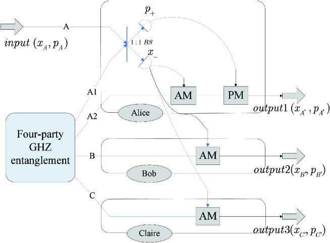
Fig. 1: The three-party position-quadrature (PQ) protocol requires a four-mode GHZ entangled state, and we label the four modes as $A_{1}$, $A_{2}$, $B$, $C$. Alice possesses mode $A_{1}$ and $A_{2}$, Bob possesses mode $B$ and Charlie possesses mode $C$. Alice has an input mode $A$ with the message to be transmitted. The elements used in this figure: AM is an amplitude modulator which displaces the position quadrature of an optical mode [3]. PM is a phase modulator which kicks the momentum quadrature of an optical mode [3]. BS is a beam splitter.

Then we present the transformations of the operators in Heisenberg picture as follows:

Step 1. Alice mixes mode $A$ and $A_{1}$ locally on a balanced (50%) beam splitter (BS), generating modes (+) and (-).

$$\begin{cases}\hat{x}_{+}=(\hat{x}_{A}+\hat{x}_{A_{1}})/\sqrt{2}\ ,\ \hat{p}_{+}=(\hat{p}_{A}+\hat{p}_{A_{1}})/\sqrt{2}\\ \hat{x}_{-}=(\hat{x}_{A}-\hat{x}_{A_{1}})/\sqrt{2}\ ,\ \hat{p}_{-}=(\hat{p}_{A}-\hat{p}_{A_{1}})/\sqrt{2}\\ \end{cases}$$ (10)

Step 2.   We denote $\hat{x}_{A_{2}}$, $\hat{p}_{A_{2}}$, $\hat{x}_{B}$ and $\hat{x}_{C}$ in terms of $\hat{x}_{-}$ and $\hat{p}_{+}$.

$$\begin{cases}{\hat{x}_{A_{2}}}&=\hat{x}_{A}-\hat{x}_{A_{1}}+\hat{x}_{A_{2}}-\sqrt{2}\hat{x}_{-}\\ \hat{p}_{A_{2}}&=\hat{p}_{A}+(\hat{p}_{A_{1}}+\hat{p}_{A_{2}}+\hat{p}_{B}+\hat{p}_{C})-\hat{p}_{B}-\hat{p}_{C}-\sqrt{2}\hat{p}_{+}\\ \hat{x}_{B}&=\hat{x}_{A}-\hat{x}_{A_{1}}+\hat{x}_{B}-\sqrt{2}\hat{x}_{-}\\ \hat{x}_{C}&=\hat{x}_{A}-\hat{x}_{A_{1}}+\hat{x}_{C}-\sqrt{2}\hat{x}_{-}\end{cases}$$ (11)

Then Alice measures $\hat{x}_{-}$ and $\hat{p}_{+}$ through the homodyne detection. After the homodyne detection, operator $\hat{x}_{-}$ and $\hat{p}_{+}$ collapse to value $x_{-}$ and $p_{+}$, then she sends the measurement value $x_{-}$ to Bob and Charlie over a classical communication channel. Suppose the photodetectors have efficiency $\eta$.

Step 3.   Alice displaces the position quadrature of her mode $A_{2}$ by $\sqrt{2}x_{-}$ and her momentum quadrature by the value of $\sqrt{2}p_{+}$, Bob and Charlie displace the position quadrature of their possessed mode B and C respectively by $\sqrt{2}x_{-}$, resulting mode $A^{\prime}$, $B^{\prime}$ and $C^{\prime}$. After the modulations, we get:

$$\begin{cases}\hat{x}_{A^{\prime}}&=\hat{x}_{A}-(\hat{x}_{A_{1}}-\hat{x}_{A_{2}})-\sqrt{2(1-\eta)/\eta}\hat{x}_{1}^{(0)}\\ \hat{p}_{A^{\prime}}&=\hat{p}_{A}+(\hat{p}_{A_{1}}+\hat{p}_{A_{2}}+\hat{p}_{B}+\hat{p}_{C})-\hat{p}_{B}-\hat{p}_{C}+\sqrt{2(1-\eta)/\eta}\hat{p}_{2}^{(0)}\\ \hat{x}_{B^{\prime}}&=\hat{x}_{A}-(\hat{x}_{A_{1}}-\hat{x}_{B})-\sqrt{2(1-\eta)/\eta}\hat{x}_{1}^{(0)}\\ \hat{p}_{B^{\prime}}&=\hat{p}_{B}\\ \hat{x}_{C^{\prime}}&=\hat{x}_{A}-(\hat{x}_{A_{1}}-\hat{x}_{C})-\sqrt{2(1-\eta)/\eta}\hat{x}_{1}^{(0)}\\ \hat{p}_{C^{\prime}}&=\hat{p}_{C}\end{cases}$$ (12)

Finally, we can find the results we obtained satisfy the constraints in (2) and (3), we get that

$$\begin{cases}\hat{x}^{\ 1}_{\Delta_{X}}=\hat{x}_{B^{\prime}}-\hat{x}_{A}=\hat{x}_{B^{\prime}}-\hat{x}_{A^{\prime}}=\hat{x}_{B}-\hat{x}_{A_{2}}\\ \hat{x}^{\ 2}_{\Delta_{X}}=\hat{x}_{C^{\prime}}-\hat{x}_{A}=\hat{x}_{C^{\prime}}-\hat{x}_{A^{\prime}}=\hat{x}_{C}-\hat{x}_{A_{2}}\\ \hat{p}_{\Delta_{X}}+\hat{p}_{B^{\prime}}+\hat{p}_{C^{\prime}}=(\hat{p}_{A_{1}}+\hat{p}_{A_{2}}+\hat{p}_{B}+\hat{p}_{C})+\sqrt{2(1-\eta)/\eta}\hat{p}_{2}^{(0)}\\ \langle\hat{x}^{\ 1}_{\Delta_{X}}\rangle=\langle\hat{x}^{\ 2}_{\Delta_{X}}\rangle=\langle\hat{p}_{\Delta_{X}}+\hat{p}_{B^{\prime}}+\hat{p}_{C^{\prime}}\rangle=0\\ \langle(\hat{x}^{\ 1}_{\Delta_{X}})^{2}\rangle\leq 2e^{-2r},\ \langle(\hat{x}^{\ 2}_{\Delta_{X}})^{2}\rangle\leq 2e^{-2r},\ \\ \langle(\hat{p}_{\Delta_{X}}+\hat{p}_{B^{\prime}}+\hat{p}_{C^{\prime}})^{2}\rangle\leq 4e^{-2r}+2(1-\eta)/\eta\end{cases}$$ (13)

So, parameters $\epsilon_{1}$, $\epsilon_{2}$ and $\epsilon_{3}$ in constraints (3) are:

$$\epsilon_{1}=\epsilon_{2}=2e^{-2r},\ \epsilon_{3}=4e^{-2r}+2(1-\eta)/\eta$$ (14)

In this case , n is equal to 3. As n increases, $\epsilon_{1}$, $\epsilon_{2}$ $\cdots$ $\epsilon_{n-1}$ remain unchanged and $\epsilon_{n}$ amounts to $(n+1)e^{-2r}+2(1-\eta)/\eta$. When it comes to the general n-party PQ conat channel in this method, we can implement it easily and similarly using the $(n+1)$-party GHZ entanglement.

The implementation of multiparty MQ conat channel is similar to multiparty PQ conat channel, viewing the operator $\hat{x}$ as $\hat{p}$ and operator $\hat{p}$ as $\hat{x}$. The required resource is a GHZ-like entanglement state with total position $\hat{x}_{A_{1}}+\hat{x}_{A_{2}}+\hat{x}_{B}+\cdots+\hat{x}_{N}\rightarrow 0$ and relative momenta equal. So we omit these discussions here.

Method 2:

Widle, Krovi and Brun proposed a protocol of coherent superdense coding recently [4]. Inspired by their work, we provide a multiparty version of coherent superdense coding. The protocol is equivalent to multiparty conat channels, a multiparty PQ conat channel and a multiparty MQ conat channel. In this method, the channel has only one sender which has two modes to be transmitted, and finally has $n$ receivers obtained the two modes respectively. In addition, $(n-1)$ prepared EPR pairs among the receivers are required.

We also use P. van Loock and S. L. Braunstein’s method to generate an EPR pair. In Heisenberg representation:

$$\begin{cases}\hat{x}_{1}=(e^{+r}\hat{x}_{1}^{(0)}+e^{-r}\hat{x}_{2}^{(0)})/\sqrt{2},\ &\hat{p}_{1}=(e^{-r}\hat{p}_{1}^{(0)}+e^{+r}\hat{p}_{2}^{(0)})/\sqrt{2}\\ \hat{x}_{2}=(e^{+r}\hat{x}_{1}^{(0)}-e^{-r}\hat{x}_{2}^{(0)})/\sqrt{2},\ &\hat{p}_{2}=(e^{-r}\hat{p}_{1}^{(0)}-e^{+r}\hat{p}_{2}^{(0)})/\sqrt{2}\end{cases}$$ (15)

Local quantum nondemolition (QND) interactions are also employed. After the transformations, we get[12]:

$$\begin{cases}\hat{x}_{1^{\prime}}=\hat{x}_{1},\ &\hat{p}_{1^{\prime}}=\hat{p}_{1}-\hat{p}_{2}\\ \hat{x}_{2^{\prime}}=\hat{x}_{1}+\hat{x}_{2},\ &\hat{p}_{2^{\prime}}=\hat{p}_{2}\end{cases}$$ (16)

The QND interaction with a phase adjust can be described as[12]:

$$\begin{cases}\hat{x}_{1^{\prime}}=\hat{x}_{1}-\hat{x}_{2},\ &\hat{p}_{1^{\prime}}=\hat{p}_{1}\\ \hat{x}_{2^{\prime}}=\hat{x}_{2},\ &\hat{p}_{2^{\prime}}=\hat{p}_{1}+\hat{p}_{2}\end{cases}$$ (17)

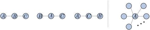
Fig. 2: On the left side of the vertical line, we present all the scenarios of graph which represents the prepared entanglement resources when n is equal to 3. The number of total scenarios is three. On the right side of the vertical line, the graph indicates the best prepared entanglement resources for n-party conat channel.

Our protocol requires $(n-1)$ EPR pairs for receivers. We illustrate these requirements in Figure 2, on the condition that $n$ equals to 3. We use a graph to illustrate the entanglement relations among the parties involved. A vertex in the graph represents an individual party in he channel, and the edge between two vertices indicates EPR entanglement relation between two parties. We will introduce concepts from graph theory: when two vertices are the terminals of a edge, they are called ’adjacent’; we refer two vertices as connected when a path exists between them; a connected graph is a graph in which any two of the vertices are connected. This method requires that the graph of entanglement resources be a connected graph. The channel has $n$ parties involved. The $(n-1)$ EPR pairs prepared among the $n$ parties ensure that the representing graph is connected, and any two vertices of the graph has only one path.

Without loss of generalization, we discuss two scenarios in Figure 2. Scenario 1 corresponds to the first graph in Figure 2, Scenario 2 corresponds to the second graph. Since $n$ is equal to 3, the channel involves one sender and three receivers, two EPR pairs is required.

Scenario 1. In this scenario, Alice and Bob shares an EPR entanglement pair: mode 3 for Alice and mode 4 for Bob, Bob and Charlie share an EPR entanglement pair: mode 5 for Bob and mode 6 for Charlie. Alice possesses mode 1 and 2 which are to be transmitted. Figure 3 gives the schematic linear optics circuit.

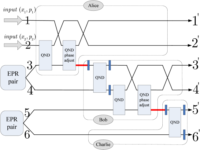
Fig. 3: This figure outlines our scheme. The thick red line in this figure represents a quantum channel between two parties. The local operations and modes are enclosed by the dashed with the name of the party. The The blue thin rectangle means the phase shifter about $\pi$.

In step 1, Alice couples her mode 2 and 3 in QND interaction, and then couples mode 1 and 3 in QND phase adjust interaction. In step 2, Alice sends her mode 3 to Bob through quantum channel, so Bob now possesses three modes, mode 3, 4 and 5. Then he performs a series of QND interactions: first couples mode 3, 4, then mode 4 and 5, finally QND phase adjust interaction about mode 3, 5. In step 3, Bob sends mode 5 to Charlie through a quantum channel. Charlie couples his two modes. then we can get the resulting modes in Heisenberg picture.

$$\begin{cases}\hat{x}_{1^{\prime}}=\hat{x}_{1}-(\hat{x}_{2}+\hat{x}_{3})\ ,\ &\hat{p}_{1^{\prime}}=\hat{p}_{1}\\ \hat{x}_{2^{\prime}}=\hat{x}_{2}\ ,\ &\hat{p}_{2^{\prime}}=\hat{p}_{2}-\hat{p}_{3}\\ \hat{x}_{3^{\prime}}=\hat{x}_{2}+\hat{x}_{3}-(\hat{x}_{2}+\hat{x}_{3}-\hat{x}_{4}+\hat{x}_{5})\,\ &\hat{p}_{3^{\prime}}=\hat{p}_{1}+\hat{p}_{3}+\hat{p}_{4}\\ \hat{x}_{4^{\prime}}=\hat{x}_{2}+\hat{x}_{3}-\hat{x}_{4}\ ,\ &\hat{p}_{4^{\prime}}=-\hat{p}_{4}-\hat{p}_{5}\\ \hat{x}_{5^{\prime}}=\hat{x}_{2}+\hat{x}_{3}-\hat{x}_{4}+\hat{x}_{5}\ ,\ &\hat{p}_{5^{\prime}}=\hat{p}_{1}+\hat{p}_{3}+\hat{p}_{4}+\hat{p}_{5}+\hat{p}_{6}\\ \hat{x}_{6^{\prime}}=\hat{x}_{2}+\hat{x}_{3}-\hat{x}_{4}+\hat{x}_{5}-\hat{x}_{6}\ ,\ &\hat{p}_{6^{\prime}}=-\hat{p}_{6}\end{cases}$$ (18)

Modes 1’, 3’, 5’ implement a three-party MQ conat channel by satisfying the constraints in definition 2; and modes 2’, 4’, 6’ satisfy definition 1 and work as a three-party PQ conat channel.

Scenario 2. In this scenario, Alice possesses four modes at the beginning: mode 1, 2, 3, 5, Bob possesses mode 4 and Charlie possesses mode 6. Mode 1 and 2 is to be transmitted while modes 3, 4, 5, 6 are the auxiliary modes. Modes 3, 4 are EPR pair, as well as modes 5, 6. We give Figure 4 to describe this protocol.

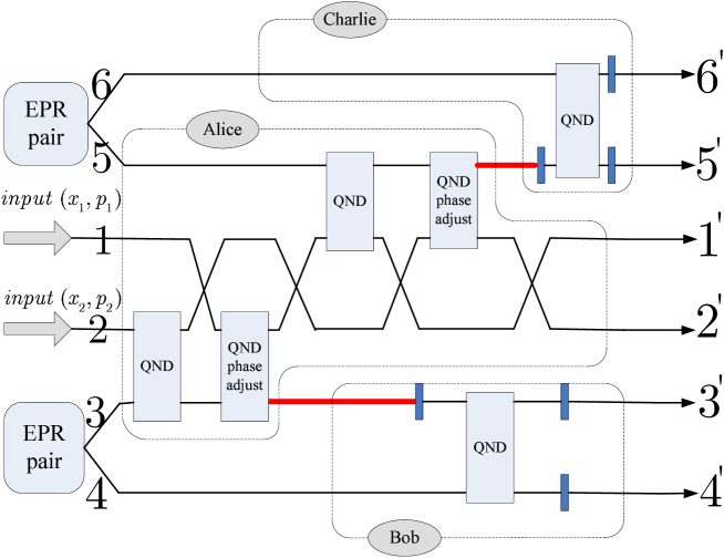
Fig. 4: The thick red line in this figure represents a quantum channel between two parties. The local operations and modes are enclosed by the dashed with the name of the party. The The blue thin rectangle means the phase shifter about $\pi$.

In step 1, Alice performs a series of QND interactions: first, couples mode 2, 3; then QND phase adjust interaction about mode 1, 3; then QND interaction between mode 2, 5; finally QND phase adjust interaction between mode 1, 5. In step 2, Alice sends mode 3 to Bob and mode 5 to Charlie through quantum channels. Then Bob possesses two modes 3, 4 and Charlie possesses modes 5, 6. They perform local QND interactions on their two modes respectively. The resulting modes are given as follows:

$$\begin{cases}\hat{x}_{1^{\prime}}=\hat{x}_{1}-(\hat{x}_{2}+\hat{x}_{3})-(\hat{x}_{2}+\hat{x}_{5})\ ,\ &\hat{p}_{1^{\prime}}=\hat{p}_{1}\\ \hat{x}_{2^{\prime}}=\hat{x}_{2}\ ,\ &\hat{p}_{2^{\prime}}=\hat{p}_{2}-\hat{p}_{3}-\hat{p}_{5}\\ \hat{x}_{3^{\prime}}=\hat{x}_{2}+\hat{x}_{3}\ ,\ &\hat{p}_{3^{\prime}}=\hat{p}_{1}+\hat{p}_{3}+\hat{p}_{4}\\ \hat{x}_{4^{\prime}}=\hat{x}_{2}+\hat{x}_{3}-\hat{x}_{4}\ ,\ &\hat{p}_{4^{\prime}}=-\hat{p}_{4}\\ \hat{x}_{5^{\prime}}=\hat{x}_{2}+\hat{x}_{5}\ ,\ &\hat{p}_{5^{\prime}}=\hat{p}_{1}+\hat{p}_{5}+\hat{p}_{6}\\ \hat{x}_{6^{\prime}}=\hat{x}_{2}+\hat{x}_{5}-\hat{x}_{6}\ ,\ &\hat{p}_{6^{\prime}}=-\hat{p}_{6}\end{cases}$$ (19)

As in scenario 1, the output modes 1’, 3’, 5’ perform a three-party MQ conat channel and modes 2’, 4’, 6’ perform a a three-party PQ conat channel. So two multiparty conat channels are produced in this protocol.

Then we discuss the noise of the channels in these two scenarios, we assume that the local QND interaction is ideal. So we get that

In Scenario 1:

$$\begin{cases}PQ\ conat\ channel&:\ \epsilon_{1}=2e^{-2r},\ \epsilon_{2}=4e^{-2r},\ \epsilon_{3}=4e^{-2r}\\ MQ\ conat\ channel&:\ \epsilon_{1}=2e^{-2r},\ \epsilon_{2}=4e^{-2r},\ \epsilon_{3}=0\end{cases}$$ (20)

In Scenario 2:

$$\begin{cases}PQ\ conat\ channel&:\ \epsilon_{1}=2e^{-2r},\ \epsilon_{2}=2e^{-2r},\ \epsilon_{3}=4e^{-2r}\\ MQ\ conat\ channel&:\ \epsilon_{1}=2e^{-2r},\ \epsilon_{2}=2e^{-2r},\ \epsilon_{3}=0\end{cases}$$ (21)

Comparing these two scenarios, we find that the noise of scenario 2 is lower. We can reach a conclusion that the longer the path between one party and Alice, the larger the noise of the party and of the channel. As you see in Figure 2, the first graph represents Scenario 1, the second graph represents Scenario 2. For instance, in Scenario 1, the length of the path between Bob and Alice is one, and the length of the path between Charlie and Alice is two. So Charlie gets larger noise $\epsilon_{2}=4e^{-2r}$. The longer the path between one party and Alice, the larger the accumulation of the noise this party gets. In Scenario 2, the length of the path between Alice and any party is one, there is no accumulation of the noise, so Scenario 2 is better. For n-party conat channel, the best prepared entanglement resources is the rightmost graph in Figure 2.

4 Conclusion

Coherent bits (cobits) are intermediate in power between qubits and cbits. Qubit sources can be used to simulate cobit sources, and cobit sources can simulate cbit sources[2]. Coherent communications offers a new view of quantum information elements.

In this paper, we extended the notion of continuous-variable coherent (conat) channel to multiparty conditions and proposed two definitions of it. Then we propose two implementations of multiparty conat channel using linear optics. One method is the multiparty version of coherent communication assisted by entanglement and classical communication (CCAECC). The other is multiparty coherent superdense coding which implements two multiparty coherent channels. We also discuss the noise of the channel in two scenarios when n equals to 3.

5 Acknowledgements

This work was supported by the National Natural Science Foundation of China (Grants No. 61102053), the Scientific Research Foundation for the Returned Overseas Chinese Scholars, State Education Ministry, SMC Excellent Young Faculty program (2011), SJTU Young Teacher Foundation (Grants No. A2831B) and SJTU PRP (Grants No. T03013002).