A bracket polynomial for graphs, IV.
Undirected Euler circuits, graph-links and multiply marked graphs

Abstract

In earlier work we introduced the graph bracket polynomial of graphs with marked vertices, motivated by the fact that the Kauffman bracket of a link diagram $D$ is determined by a looped, marked version of the interlacement graph associated to a directed Euler system of the universe graph of $D$. Here we extend the graph bracket to graphs whose vertices may carry different kinds of marks, and we show how multiply marked graphs encode interlacement with respect to arbitrary (undirected) Euler systems. The extended machinery brings together the earlier version and the graph-links of D. P. Ilyutko and V. O. Manturov [J. Knot Theory Ramifications 18 (2009), 791-823]. The greater flexibility of the extended bracket also allows for a recursive description much simpler than that of the earlier version.

Keywords. circuit partition, graph, graph-link, interlacement, Jones polynomial, Kauffman bracket, local complement, Reidemeister move, virtual link

2000 Mathematics Subject Classification. 57M25, 05C50

1 Introduction

An oriented link diagram is a finite collection of oriented, piecewise smooth closed curves in the plane, whose only singularities are finitely many crossings (double points). Classical crossings may be positive or negative, as indicated in Fig. 1, and there may also be virtual crossings. On the rare occasion when we want to restrict attention to diagrams without virtual crossings, we refer to classical diagrams or classical links.

Figure 1: The smoothings of classical crossings.

The Kauffman bracket of an oriented link diagram $D$ is defined by a formula that incorporates the numbers of closed curves in the various Kauffman states of $D$ [18, 19]. If $D$ has $n$ classical crossings then it has $2^{n}$ states, obtained by choosing one of the two smoothings at each classical crossing; see Fig. 1. The bracket is then

$$[D]=\sum_{S}A^{a(S)}B^{b(s)}d^{c(S)-1},$$

in which the contribution of each state $S$ is determined by the number $a(S)$ of $A$ smoothings in $S$, the number $b(S)$ of $B$ smoothings in $S$, and the number $c(S)$ of closed curves in $S$. We use $[D]$ rather than the more familiar notation $\left\langle D\right\rangle$ in order to distinguish this three-variable bracket polynomial from its reduced one-variable form.

Associated to an oriented link diagram $D$ there is a 4-regular graph $U$, the universe graph of $D$, whose vertices correspond to the classical crossings of $D$ and whose edges correspond to the arcs of $D$. Each vertex of $U$ carries the sign of the corresponding crossing of $D$. The 2-in, 2-out directed graph obtained from $U$ by directing its edges in accordance with the orientations of the link components is denoted $\vec{U}$. It should be emphasized that although $D$ is given as a specific subset of the plane, we regard $U$ and $\vec{U}$ as abstract (nonimbedded) graphs, with signed vertices. For the universe (di)graphs of two diagrams to be isomorphic (informally, the same) there must be a one-to-one correspondence between their vertices that preserves not only edges but also vertex signs; the correspondence need not be compatible with the way the diagrams are drawn in the plane.

If $D$ is a diagram of a knot $K$ then it has a looped interlacement graph $\mathcal{L}(D)$, i.e. the graph whose vertices correspond to the classical crossings of $D$ and whose edges are defined by (a) a vertex is looped if and only if the corresponding crossing is negative and (b) two distinct vertices are adjacent if and only if the corresponding crossings are interlaced on $K$, i.e. when we follow $K$ around $D$ we encounter first one of the two crossings, then the second, then the first again, and then the second again. See Fig. 2 for an example. (As usual, the encircled crossing is virtual.)

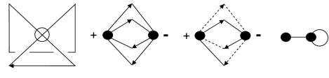
Figure 2: A trivial knot diagram $D$, the directed universe $\vec{U}$, the Euler circuit determined by the knot, and $\mathcal{L}(D)$. When following the Euler circuit determined by the knot, we traverse each vertex without changing the pattern of dashes.

The looped interlacement graph was introduced in the first paper of this series [36], where Zulli and the present author showed that if $D$ is a classical or virtual knot diagram then $\mathcal{L}(D)$ contains enough information about the states of $D$ to determine both the Kauffman bracket $[D]$ and the Jones polynomial $V_{D}$ [17]. As $\mathcal{L}(D)$ is determined by the abstract graph $\vec{U}$ and the Euler circuit of $\vec{U}$ that corresponds to the diagrammed knot, this provides a striking conceptual simplification of the Kauffman brackets and Jones polynomials of knots: if $D$ and $D^{\prime}$ are knot diagrams with the same universe digraph $\vec{U}=\overrightarrow{U^{\prime}}$, and the knots diagrammed in $D$ and $D^{\prime}$ correspond to the same Euler circuit, then $[D]=[D^{\prime}]$ and $V_{D}=V_{D^{\prime}}$. (To say the same thing in a different way: if two knot diagrams $D$ and $D^{\prime}$ represent immersions in the plane of the same abstract directed graph $\vec{U}$, with the same Euler circuit of $\vec{U}$ corresponding to both diagrammed knots and every pair of crossings corresponding to the same vertex having the same sign, then $[D]=[D^{\prime}]$ and $V_{D}=V_{D^{\prime}}$.) For instance, in [19] Kauffman mentioned that the virtual knot diagram $D$ that appears at the top left in Fig. 3 has $V_{D}=1$, even though $D$ is not a diagram of the unknot. As indicated in the figure, its $\vec{U}$ and $\mathcal{L}(D)$ are isomorphic to those of an unknot diagram. Indeed, every classical or virtual knot diagram with $V_{D}=1$ that we have seen has $\vec{U}$ and $\mathcal{L}(D)$ isomorphic to those of an unknot diagram.

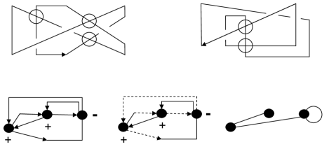
Figure 3: A nontrivial knot diagram and a trivial knot diagram give rise to the same directed universe graph. The two knots determine the same Euler circuit and (hence) the same looped interlacement graph.

As discussed in [36], if we think of the Kauffman bracket $[D]$ as a function of $\mathcal{L}(D)$ then this function may be extended to arbitrary graphs. The extended function is called the graph bracket polynomial, and it resembles the Kauffman bracket of virtual knot diagrams in several ways, including the fact that it yields a graph Jones polynomial which is invariant under graph operations suggested by the Reidemeister moves.

If $D$ is a diagram of an oriented multi-component link rather than a knot, then $[D]$ can still be determined by using interlacement in $\vec{U}$, as discussed in the second paper in this series [34]. The situation is complicated by the fact that $U$ need not be connected, so interlacement is defined with respect to a directed Euler system $C$ of $\vec{U}$, i.e. a set containing a directed Euler circuit for each connected component of $\vec{U}$. Directed Euler systems certainly exist, but there is no canonical way to choose a preferred one. Also, $D$ may contain link components that have no classical crossings and hence are not detected by $U$; such link components certainly affect $[D]$. These complications are handled by modifying $\vec{U}$ and $\mathcal{L}$ to incorporate additional information. First, $\vec{U}$ is modified to include a free loop corresponding to each link component without any classical crossing. Free loops are essentially empty connected components; they contain neither vertices nor edges but they contribute to $c(U)$, the number of connected components of $U$. The modified interlacement graph $\mathcal{L}(D$, $C)$ includes $c(U)-1$ free loops. The relationship between $C$ and the link diagrammed in $D$ is recorded by marking the crossings of $D$ at which $C$ does not follow the incident link component(s); the marks are transferred to the corresponding vertices of $\vec{U}$ and $\mathcal{L}(D$, $C)$, and isomorphisms are required to preserve free loops, vertex marks and vertex signs. As before, the description of $[D]$ as a function of $\mathcal{L}(D$, $C)$ extends directly to a bracket polynomial defined for any graph that may include free loops and marked vertices, and this bracket polynomial gives rise to a marked-graph Jones polynomial that is invariant under the appropriate versions of the Reidemeister moves [34, 35].

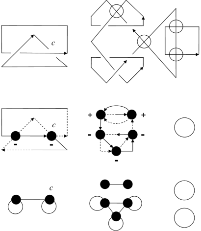
Figure 4: A marked link diagram $D$, the directed universe $\vec{U}$ with an Euler system $C$ indicated by dashes, and $\mathcal{L}(D,C)$. The circuits of $C$ are consistent with the orientations of the link components.

These definitions are illustrated in Fig. 4. The top row is a diagram $D$ of an oriented link with four link components; virtual crossings are encircled as usual. The mark $c$ on a crossing of $D$ specifies the Euler system of $\vec{U}$ indicated by dashes. (That is, whenever we follow the Euler circuit through a vertex we do not change the pattern of dashes.) $\vec{U}$ is a 2-in, 2-out digraph with two nonempty connected components. One nonempty connected component of $\vec{U}$ is pictured so as to resemble the corresponding portion of $D$, and the other nonempty connected component is not; as $\vec{U}$ is an abstract graph, we may picture it however we please. $\vec{U}$ has a free loop corresponding to the crossing-less link component of $D$; the free loop is indicated by a vertex-less circle. $\mathcal{L}(D$, $C)$ has looped vertices corresponding to negative crossings of $D$, and it has two free loops because $c(U)=3$. The factors of the connected sum (the link’s one knotted component) are not interlaced, so the two nonempty connected components of $U$ give rise to three nonempty connected components in $\mathcal{L}(D$, $C)$. The only difference between $\mathcal{L}(D$, $C)$ and the interlacement graph of a diagram $D^{\prime}$ obtained from $D$ by splitting the connected sum into separate parts is that $\mathcal{L}(D^{\prime}$, $C)$ has more free loops.

Thistlethwaite [32] observed that the Kauffman bracket provides a connection between knot theory (in particular, the Jones polynomials and Kauffman brackets of classical links) and combinatorial theory (in particular, the Tutte polynomial of planar graphs). Underlying Thistlethwaite’s theorem is a connection between circuit partitions of 4-regular plane graphs and Tutte polynomials of their associated checkerboard graphs that was actually discovered before the introduction of the Jones polynomial and Kauffman bracket [16, 22, 23]. A useful technique in establishing this connection involves giving a 4-regular plane graph an alternating orientation (or “source-sink orientation” in the terminology of [24]), i.e. directing the edges so that the boundary of each complementary region is coherently oriented, with (say) the boundaries of white-colored regions oriented clockwise and the boundaries of black-colored regions oriented counterclockwise. (The same technique has also been of use in connection with the interlace polynomial of Arratia, Bollobás and Sorkin [1, 2, 10].) If $D$ is a diagram of an oriented classical link then clearly such a re-oriented version of $U$ is inconsistent with the link components, in the sense that we cannot follow a link component through any vertex without disregarding edge-directions. Directed Euler circuits of this re-oriented version of $U$ have been called bent Euler tours [12], rotating circuits [13, 14, 15], $\sigma$-lines [21] and non-crossing Euler tours [22].

Interlacement with respect to rotating circuits is the fundamental notion of Ilyutko’s and Manturov’s theory of graph-links, a relative of the theory of looped interlacement graphs outlined above. Just as the looped graphs considered in the first paper in this series were motivated by knot diagrams, the first graph-links were motivated by link diagrams associated with geometric structures called orientable atoms [14]. Both theories have grown more general since they were introduced, and may now be used with arbitrary link diagrams; however they are not quite the same. The graph-link theory is motivated by interlacement with respect to rotating circuits [15], and the marked-graph theory, instead, is motivated by interlacement with respect to Euler systems that respect the orientations of the link components [34]. This difference is reflected in the fact that the writhe of a marked graph is quite a simple notion – just subtract the number of looped vertices from the number of unlooped vertices – while there is no such simple notion of writhe for a graph-link. Ilyutko [13] has proven that the Reidemeister equivalence classes of graphs defined in [36] correspond precisely to graph-knots (i.e. the graph-links for which the sum of the adjacency matrix and an identity matrix is invertible), but it is not clear whether or not this equivalence extends to the general case.

Our purpose in the present paper is to extend the marked-graph machinery to allow interlacement with respect to arbitrary Euler systems of $U$, thereby developing a single theory that brings together graph-links and marked graphs. In Section 2 we explain how to associate a marked interlacement graph $\mathcal{L}(D,C)$ to an arbitrary Euler system $C$ in the universe graph of a link diagram $D$; six different kinds of marks are used to record the different ways an Euler system can pass through a crossing. The various marked interlacement graphs that result from choosing different Euler systems in $D$ are related to each other through a marked version of local complementation, the fundamental operation of the theory of circle graphs [21, 30]. Our vertex marks involve the letters $c$, $r$ and $u$, so we use $G_{cru}^{v}$ to denote the marked local complement of $G$. In Section 3 we discuss marked-graph versions of the Reidemeister moves. In Section 4 we define the bracket polynomial of a marked graph, and show that it is invariant under marked local complementation. If $D$ is a link diagram then the Kauffman bracket $[D]$ is the same as the marked-graph bracket $[\mathcal{L}(D,C)]$. The marked-graph version of the Jones polynomial [17], $V_{G}$, is obtained from the bracket $[G]$ in the usual way, i.e. by evaluating $B\mapsto A^{-1}$ and $d\mapsto-A^{2}-A^{-2}$, and then multiplying by a factor given by the writhe and the number of vertices. The marked-graph Jones polynomial is invariant under the marked-graph Reidemeister moves. In Sections 5 and 6 we discuss the relationship between graph-links and marked graphs.

The Kauffman bracket of a (virtual) link diagram is recursively calculated by eliminating classical crossings one at a time, applying the formula $[D]=A[D_{A}]+B[D_{B}]$ at each step [18, 19]. The marked-graph bracket polynomial of [34, 36] is calculated using a recursive algorithm that is considerably more complicated: different recursive steps are applied in different circumstances, according to the placement of loops and marks. It turns out, though, that using marked local complementation we can also devise a much simpler algorithm, similar to that of the Kauffman bracket.

Theorem 1

The marked-graph bracket polynomial of a marked graph $G$ can be calculated recursively using the following properties.

(a) The bracket polynomial of the empty graph is $[\emptyset]=1$, and the bracket polynomial of a 1-vertex graph is given by the following.

$$[(v)]=[(v,r,\ell)]=Ad+B=[(v,u)]=[(v,ur,\ell)]$$

$$[(v,\ell)]=[(v,r)]=A+Bd=[(v,u,\ell)]=[(v,ur)]$$

$$[(v,c)]=[(v,cr,\ell)]=A+B=[(v,c,\ell)]=[(v,cr)]$$

Here $(v)$ indicates that $v$ is unlooped and unmarked, $(v,\ell)$ indicates that $v$ is looped and unmarked, $(v,cr)$ indicates that $v$ is unlooped and marked $cr$, $(v,u,\ell)$ indicates that $v$ is looped and marked $u$, and so on.

(b) If $G^{\prime}$ is obtained from $G$ by removing a free loop then $[G]=d\cdot[G^{\prime}]$.

(c) If $G^{\prime}$ is obtained from $G$ by removing an isolated vertex $v$ then $[G]=[\{v\}]\cdot[G^{\prime}]$; $[\{v\}]$ is given in part (a).

(d) If the vertex $v$ is unlooped and marked $c$, or looped and marked $cr$, then

$$[G]=A[G-v]+B[G_{cru}^{v}-v],$$

where $G_{cru}^{v}$ is the marked local complement of $G$ with respect to $v$. On the other hand, if $v$ is looped and marked $c$, or unlooped and marked $cr$, then

$$\text{\ }[G]=B[G-v]+A[G_{cru}^{v}-v].$$

(e) If $v$ has a neighbor marked $u$ or $ur$ then $[G]=[G_{cru}^{v}]$.

(f) If the vertex $w$ is unmarked or marked $r$ then $[G]=[G_{cru}^{w}]$.

Despite having six options, Theorem 1 is quite similar to the Kauffman bracket’s recursion. Parts (a) – (c) correspond to simple properties involving very small portions of link diagrams, and part (d) corresponds to the formula $[D]=A[D_{A}]+B[D_{B}]$. At first glance parts (e) and (f) may seem to be novel complications, but it is important to remember that Theorem 1 is applied to abstract graphs and the Kauffman bracket, instead, is applied to plane diagrams. When we draw $D$ in the plane, we know which transition to call $A$ and which transition to call $B$ at each crossing; and when we smooth a crossing to obtain $D_{A}$ and $D_{B}$, these new diagrams are drawn in the plane so as to guarantee appropriate choices of $A$ and $B$ smoothings at the remaining crossings. Similarly, the use of marked local complementations in (e) and (f), together with the restriction of (d) to vertices marked $c$ or $cr$, ensures that when we replace an abstract graph $G$ with smaller abstract graphs during the recursion, the smaller graphs inherit the appropriate $A$ and $B$ assignments.

At the end of the paper we briefly discuss appropriate modifications of the results of [35], involving the use of vertex weights in streamlining bracket calculations.

Figure 5: A chord diagram representing the Euler system of Fig. 4.

Before beginning a detailed discussion we recall that Euler systems of 4-regular graphs are equivalent to two other familiar combinatorial structures: double occurrence words and chord diagrams. For instance, the Euler system of Fig. 4 could be represented by the word $bcbcdefghfghde$, or by the chord diagram in Fig. 5. (In order to carry as much information as Fig. 4 does, the double occurrence word or chord diagram should incorporate the vertex signs and marks.) Although these three kinds of structures are equivalent to each other, we prefer to use Euler systems in 4-regular graphs. Our first reason for this preference is the obviousness of the observation that a typical 4-regular graph has many different Euler systems; the equivalence relations on double occurrence words and chord diagrams motivated by this obvious observation are not so intuitively immediate. Our second reason is the richness of the combinatorial theory of 4-regular graphs, which has been developed by Bouchet, Jaeger, Las Vergnas, Martin and others in the decades since Kotzig’s foundational work [21]. We believe this beautiful theory will prove to be of great interest to knot theorists. In particular, Bouchet’s comment that “the theory of isotropic systems is the theory of simple graphs up to local complementations” [3] makes it seem likely that much of our machinery could be re-cast using marked versions of isotropic systems or multimatroids [5].

2 Interlacement and local complementation

Figure 6: The six ways an Euler system might be related to a link at a crossing.

Suppose $D$ is an oriented link diagram, $U$ is the undirected universe graph and $C$ is an arbitrary Euler system of $U$, i.e. $C$ contains one Euler circuit for each connected component of $U$. At each vertex there are six different ways the incident circuit of an undirected Euler system $C$ might be related to the incident link component(s). See Fig. 6. Note that the edge-directions in the figure do not agree: those in the top row refer to the orientations of the link components, and those in the two lower rows refer to an orientation of the incident circuit of $C$. We do not regard the circuits of an Euler system as carrying preferred orientations, so each circuit can be oriented in either of the two possible ways. Consequently the two lower rows of Fig. 6 picture six cases, not twelve; the two in each column are the same. The six cases fall into three pairs, indicated by the letter $r$ (for rotate).

These considerations motivate the following definitions.

Definition 2

A graph is multiply marked by assigning to each of its vertices one of the six labels of Figure 6.

We often use marked rather than multiply marked; when we want to focus attention on the special cases considered in [34, 35, 36] we say unmarked or singly marked.

Definition 3

Let $D$ be an oriented link diagram, and let $C$ be an Euler system $C$ of the universe graph $U$. The vertices of $U$ are assigned marks and signs as in Figure 6, and the marked interlacement graph $\mathcal{L}(D$, $C)$ is defined as follows.

1. Vertices correspond to classical crossings of $D$. They are assigned marks as in Fig. 6.

2. A vertex is looped if and only if the corresponding crossing is negative.

3. Two distinct vertices are adjacent if and only if they are interlaced with respect to $C$.

4. $\mathcal{L}(D$, $C)$ has $c(U)-1$ free loops.

Definition 4

The writhe of a graph $G$ with $n$ vertices and $\ell$ looped vertices is $w(G)=n-2\ell$.

Fig. 7 shows the result of applying these definitions to the example of Fig. 4, with a different Euler system. To keep the figure simple, the signs of the negative vertices of $U$ are not indicated. Note also that the arc-directions in $D$ reflect the orientations of the link components, but the edge-directions in $U$ reflect a choice of orientations for the Euler circuits in $C$.

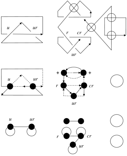
Figure 7: A marked link diagram $D$, the universe $U$ with an Euler system $C$ indicated by dashes, and $\mathcal{L}(D,C)$. The edge-directions and patterns of dashes in $U$ indicate walks along the circuits of $C$; they are not consistent with the link components. To reduce clutter, signs are indicated only for the two positive vertices of $U$.

If $C$ is an Euler system of $G$ and $v\in V(G)$ then Kotzig [21] defined the $\kappa$-transform $C\ast v$ to be the Euler system obtained from $C$ by reversing one of the two $v$-to-$v$ paths in the Euler circuit of $C$ incident on $v$, and he proved that the various Euler systems of a 4-regular graph $G$ are all related to each other through $\kappa$-transformations. (A proof appears in [34].) We do not regard Euler systems as carrying preferred orientations, so it does not matter which of the two $v$-to-$v$ paths is reversed. The effect of a $\kappa$-transformation on interlacement is easy to see: the only interlacements that are changed are those that involve two vertices both of which appear precisely once on each $v$-to-$v$ path of $C$, i.e. both of which are interlaced with $v$; the effect of the $\kappa$-transformation is to toggle (reverse) the interlacement of every such pair. Consequently, the effect of a $\kappa$-transformation $C\ast v$ on vertices of the interlacement graph other than than $v$ itself is partly described by local complementation.

Figure 8: $C$ and $C\ast v$.

Definition 5

If $G$ is a graph and $v\in V(G)$ then the local complement $G^{v}$ is the graph obtained from $G$ by toggling edges involving only neighbors of $v$. That is, if $w\neq v$ is adjacent to $v$ then $w$ is looped in $G^{v}$ if and only if it is not looped in $G$; and if $v\neq x\neq y\neq v$ and $x$, $y\,$ are both neighbors of $v$ then $x$, $y$ are adjacent in $G^{v}$ if and only if they are not adjacent in $G$.

Observe that this definition involves changes to both loops and non-loop edges. A different definition, which is intended for simple graphs and consequently affects only non-loop edges, also appears in the combinatorial literature.

Read and Rosenstiehl [30] noted that for unlooped, unmarked interlacement graphs, simple local complementation at $v$ completely describes the effect of a $\kappa$-transformation at $v$. For us, however, this is not quite true, because local complementation does not have the correct effect on the vertex marks of neighbors of $v$: if $v$ and $w$ are interlaced with respect to $C$ then in $C\ast v$ the direction of one passage through $w$ is reversed, and looking at Fig. 6 we see that this changes the vertex-mark of $w$ according to the pairings $ur\leftrightarrow c$, $u\leftrightarrow cr$, $r\leftrightarrow$(unmarked). Moreover, a $\kappa$-transformation at $v$ affects the mark of $v$ itself, as illustrated in Fig. 9. Taking these effects into account, we are led to the next definition.

Figure 9: The effect of a $\kappa$-transformation on the vertex where it is performed.

Definition 6

If $G$ is a marked graph and $v\in V(G)$ then the marked local complement $G_{cru}^{v}$ is the graph obtained from $G$ by making the following changes, and no others.

1. If $v$ is unmarked in $G$ then it is marked $u$ in $G_{cru}^{v}$, and vice versa.

2. If $v$ is marked $r$ in $G$ then it is marked $ur$ in $G_{cru}^{v}$, and vice versa.

3. If $v$ is marked $c$ in $G$ then it is marked $cr$ in $G_{cru}^{v}$, and vice versa.

4. If $w\neq v$ is an unmarked neighbor of $v$ in $G$ then $w$ is marked $r$ in $G_{cru}^{v}$, and vice versa.

5. If $w\neq v$ is a neighbor of $v$ marked $c$ in $G$, then $w$ is marked $ur$ in $G_{cru}^{v}$, and vice versa.

6. If $w\neq v$ is a neighbor of $v$ marked $u$ in $G$, then $w$ is marked $cr$ in $G_{cru}^{v}$, and vice versa.

7. If $v\neq x\neq y\neq v$ and $x$, $y\,$ are both neighbors of $v$ then $x$, $y$ are adjacent in $G_{cru}^{v}$ if and only if they are not adjacent in $G$.

Note that unlike Definition 5, Definition 6 does not involve any loop-toggling, and consequently $w(G)=w(G_{cru}^{v})$. Definition 6 is the culmination of a rather long process of understanding the effect on interlacement of changing Euler systems in link diagrams. [36] did not require changing Euler circuits at all, and [14] and [34] both required some changing of Euler circuits, but could use appropriate modifications of the more specialized pivot operation. (As discussed below, a pivot is expressible as a composition of local complementations; the reverse is not true in general.) It was the appearance of a modified local complement operation in [15] that inspired the approach we take here.

If $D$ is a link diagram then Kotzig’s theorem [21] tells us that all the Euler systems of $U$ are related to each other through $\kappa$-transformations. As the marked interlacement graph of $\mathcal{L}(D$, $C\ast v)$ is the marked local complement $\mathcal{L}(D$, $C)_{cru}^{v}$, we conclude that the marked interlacement graphs of $D$ are all related to each other through marked local complementations.

Theorem 7

Let $D$ be an oriented link diagram with a marked interlacement graph $G=\mathcal{L}(D$, $C)$, and suppose $G^{\prime}$ is an arbitrary marked graph. Then $G^{\prime}=\mathcal{L}(D$, $C^{\prime})$ for some Euler system $C^{\prime}$ of $D$ if and only if $G^{\prime}$ can be obtained from $G$ through marked local complementations.

We close this section by extending the marked pivot operation of [34] to multiply marked graphs.

Lemma 8

Suppose $G$ is a marked graph with two adjacent vertices $v\neq w$. Let $N_{v}$ be the set of neighbors of $v$ that are not neighbors of $w$, $N_{w}$ the set of neighbors of $w$ that are not neighbors of $v$, and $N_{vw}$ the set of neighbors shared by $v$ and $w$; in particular, $v\in N_{w}$ and $w\in N_{v}$. Then $((G_{cru}^{v})_{cru}^{w})_{cru}^{v}$ is the graph obtained from $G$ by making the following changes, and no others.

(a) The mark on $v$ is changed according to the pattern $c\leftrightarrow$(unmarked), $r\leftrightarrow cr$, $u\leftrightarrow ur$.

(b) The mark of $w$ is changed according to the same pattern.

(c) The neighbors of $v$ in $((G_{cru}^{v})_{cru}^{w})_{cru}^{v}$ are the elements of $(N_{w}-v)\cup\{w\}\cup N_{vw}$ and the neighbors of $w$ in $((G_{cru}^{v})_{cru}^{w})_{cru}^{v}$ are the elements of $(N_{v}-w)\cup\{v\}\cup N_{vw}$.

(d) Every adjacency involving two vertices from different elements of $\{N_{v}-w$, $N_{w}-v$, $N_{vw}\}$ is toggled.

Proof. Definition 6 tells us that the three local complementations affect the mark of $v$ as follows: $c\leftrightarrow cr\leftrightarrow u\leftrightarrow$(unmarked), $r\leftrightarrow ur\leftrightarrow c\leftrightarrow cr$ and $u\leftrightarrow$(unmarked)$\leftrightarrow r\leftrightarrow ur$. The three local complementations affect the mark of $w$ as follows: $c\leftrightarrow ur\leftrightarrow r\leftrightarrow$(unmarked), $r\leftrightarrow$(unmarked)$\leftrightarrow u\leftrightarrow c$, and $u\leftrightarrow cr\leftrightarrow c\leftrightarrow ur$.

Part (c) is verified as follows. Observe first that the neighbor-sets of vertices outside $N_{v}\cup N_{w}\cup N_{vw}$ are not affected by local complementations at $v$ and $w$, and $v$ and $w$ remain neighbors through all three local complementations. If $x\in N_{v}-w$ then $x$ is adjacent to both $v$ and $w$ in $G_{cru}^{v}$, so $x$ is adjacent to $w$ and not $v$ in $(G_{cru}^{v})_{cru}^{w}$; this remains the same in $((G_{cru}^{v})_{cru}^{w})_{cru}^{v}$. If $x\in N_{w}-v$ then $x$ is adjacent to $w$ and not $v$ in $G_{cru}^{v}$, so $x$ is adjacent to both $v$ and $w$ in $(G_{cru}^{v})_{cru}^{w}$, so $x$ is adjacent to $v$ and not $w$ in $((G_{cru}^{v})_{cru}^{w})_{cru}^{v}$. If $x\in N_{vw}$ then $x$ is adjacent to $v$ and not $w$ in $G_{cru}^{v}$, so $x$ is adjacent to $v$ and not $w$ in $(G_{cru}^{v})_{cru}^{w}$, so $x$ is adjacent to $v$ and $w$ in $((G_{cru}^{v})_{cru}^{w})_{cru}^{v}$.

For part (d), if $x\in N_{v}-w$ and $y\in N_{w}-v$ then the adjacency between $x$ and $y$ is unchanged in $G_{cru}^{v}$, then toggled in $(G_{cru}^{v})_{cru}^{w}$, and then unchanged in $((G_{cru}^{v})_{cru}^{w})_{cru}^{v}$. If $x\in N_{v}-w$ and $y\in N_{vw}$ then the adjacency between $x$ and $y$ is toggled in $G_{cru}^{v}$, then unchanged in $(G_{cru}^{v})_{cru}^{w}$, and then unchanged in $((G_{cru}^{v})_{cru}^{w})_{cru}^{v}$. If $x\in N_{w}-v$ and $y\in N_{vw}$ then the adjacency between $x$ and $y$ is unchanged in $G_{cru}^{v}$, unchanged in $(G_{cru}^{v})_{cru}^{w}$, and then toggled in $((G_{cru}^{v})_{cru}^{w})_{cru}^{v}$.

It remains to verify that no other change is made. If $x\notin N_{v}\cup N_{w}\cup N_{vw}$ then none of the local complementations affects the mark of $x$, or any adjacency involving $x$. If $x\neq y$ are in the same one of $N_{v}-w$, $N_{w}-v$, $N_{vw}$ then their adjacency is toggled by two of the three local complementations, so it remains unchanged in $((G_{cru}^{v})_{cru}^{w})_{cru}^{v}$. If $x\in N_{v}-w$ then its mark is affected as follows: $c\rightarrow ur\rightarrow c\rightarrow c$, $cr\rightarrow u\rightarrow cr\rightarrow cr$, $u\rightarrow cr\rightarrow u\rightarrow u$, $ur\rightarrow c\rightarrow ur\rightarrow ur$, $r\rightarrow$(unmarked)$\rightarrow r\rightarrow r$ , and (unmarked)$\rightarrow r\rightarrow$(unmarked)$\rightarrow$(unmarked). If $x\in N_{w}-v$ then its mark is affected as follows: $c\rightarrow c\rightarrow ur\rightarrow c$, $cr\rightarrow cr\rightarrow u\rightarrow cr$, $u\rightarrow u\rightarrow cr\rightarrow u$, $ur\rightarrow ur\rightarrow c\rightarrow ur$, $r\rightarrow r\rightarrow$(unmarked)$\rightarrow r$, and (unmarked)$\rightarrow$(unmarked)$\rightarrow r\rightarrow$(unmarked). Finally, if $x\in N_{vw}$ then its mark is affected as follows: $c\rightarrow ur\rightarrow ur\rightarrow c$, $cr\rightarrow u\rightarrow u\rightarrow cr$, $u\rightarrow cr\rightarrow cr\rightarrow u$, $ur\rightarrow c\rightarrow c\rightarrow ur$, $r\rightarrow$(unmarked)$\rightarrow$(unmarked)$\rightarrow r$, and (unmarked)$\rightarrow r\rightarrow r\rightarrow$(unmarked).   

Definition 9

Let $G$ be a doubly marked graph with two adjacent vertices $v\neq w$. Then the graph $((G_{cru}^{v})_{cru}^{w})_{cru}^{v}$ is the marked pivot of $G$ with respect to $v$ and $w$, denoted $G_{cru}^{vw}.$

The unmarked version of Definition 9 is the equality $((G^{v})^{w})^{v}=G^{vw}$ relating local complements and pivots. This equality is a familiar part of the theory of local complementation; see for instance [2, 5]. As mentioned in [2], the unmarked version of part (c) of Lemma 8 is unnecessary; up to isomorphism, simply exchanging of the names of $v$ and $w$ has the same effect. We include (c) because omitting it would require more complicated versions of (a) and (b).

3 Reidemeister equivalence

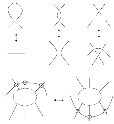
Figure 10: Three classical Reidemeister moves above a detour move.

Recall that diagrams representing the same virtual link type are obtained from each other by using both classical Reidemeister moves that involve only classical crossings, and virtual Reidemeister moves that involve virtual crossings. As noted in [11], the virtual Reidemeister moves may be subsumed in the more general detour move: any arc containing no classical crossing may be replaced by any other arc with the same endpoints, provided that the only singularities on the new arc are finitely many double points, and these double points are all designated as virtual crossings. See Fig. 10. It is obvious that detour moves on $D$ have no effect on $\mathcal{L}(D,C)$.

The effects of classical Reidemeister moves on singly marked interlacement graphs were described in [34, 36], using an elegant idea due to Östlund [26]: explicit descriptions of all possible moves are not required, so long as we describe sufficiently many moves to generate the rest through composition.

The first kind of Reidemeister move from [34] involves adjoining or deleting an unmarked, isolated vertex; the vertex may be looped or unlooped. Using marked local complementation, an unmarked isolated vertex is transformed into an isolated vertex marked $u$. It is not possible to obtain an isolated vertex with any other mark. This reflects the fact that there are only two ways an Euler circuit can traverse a trivial crossing in a link diagram; see Fig. 11.

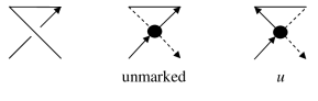
Figure 11: The two ways an Euler circuit can traverse a trivial crossing.

Definition 10

An $\Omega.1$ move is performed by adjoining or removing an isolated vertex whose mark does not involve $c$ or $r$. The vertex may be looped or unlooped.

Four kinds of $\Omega.2$ moves are explicitly described in [34].

Definition 11

Suppose $G$ is a marked graph with two vertices $v$ and $w$, $v$ looped and $w$ not looped. Then any of the following is an $\Omega.2$ move, and so is the inverse transformation.

(a) Suppose $v$ and $w$ are both unmarked, and they have the same neighbors outside $\{v$, $w\}$. Replace $G$ with $G-v-w$.

(b) Suppose $v$ is marked $c$, $w$ is unmarked, $v$ is the only neighbor of $w$, and $z\notin\{v$, $w\}$ is a neighbor of $v$. Replace $G$ with $G_{cru}^{vz}-v-w$.

(c) Suppose $v$ is marked $c$, $w$ is unmarked, $v$ and $w$ have the same neighbors outside $\{v$, $w\}$, and $z\notin\{v$, $w\}$ is a neighbor of $v$ and $w$. Replace $G$ with $G_{cru}^{vz}-v-w$.

(d) Suppose $v$ is marked $c$, $w$ is unmarked, $v$ is the only neighbor of $w$, and $w$ is the only neighbor of $v$. Replace $G$ with $G^{+}-v-w$, where $G^{+}$ is obtained from $G$ by adjoining a free loop.

Only one kind of $\Omega.3$ move is explicitly described in [34].

Definition 12

Suppose $G$ is a marked graph with three unmarked vertices $u$, $v$, $w$ such that $u$, $v$, $w$ are all adjacent to each other, $u$ is looped, $v$ and $w$ are unlooped, and every vertex $x\notin\{u$, $v$, $w\}$ is adjacent to either none or precisely two of $u$, $v$, $w$. An $\Omega.3$ move is performed by replacing $G$ with the graph obtained by removing all three edges $\{u$, $v\}$, $\{u$, $w\}$ and $\{v$, $w\}$.

The inverse of an $\Omega.3$ move is also an $\Omega.3$ move, as is the composition of an $\Omega.3$ move with $\Omega.2$ moves. Moreover the “mirror image” of an $\Omega.3$ move – i.e. the transformation obtained by first toggling all loops, then applying an $\Omega.3$ move, and then toggling all loops again – is also an $\Omega.3$ move. There are many different resulting moves, including the six from [36] pictured in Fig. 12.

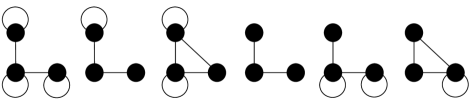
Figure 12: If every unpictured vertex is adjacent to either none or precisely two of the three pictured vertices in one of these six configurations, an $\Omega.3$ move may be performed by toggling all non-loop edges among the three pictured vertices.

Theorem 7 tells us how to extend the Reidemeister moves of [34, 36] from singly marked graphs to multiply marked graphs: simply compose with marked local complementations.

Definition 13

A marked-graph Reidemeister move on a marked graph $G$ is performed by first applying marked local complementations, then applying one of the marked-graph Reidemeister moves defined above, and then applying marked local complementations.

Two marked graphs are Reidemeister equivalent if they can be obtained from each other using marked local complementations and marked-graph Reidemeister moves.

Theorem 14

Let $D$ and $D^{\prime}$ be oriented link diagrams representing the same virtual link type. Then for any Euler systems $C$ and $C^{\prime}$ of the corresponding universe graphs, $\mathcal{L}(D^{\prime}$, $C^{\prime})$ can be obtained from $\mathcal{L}(D$, $C)$ by using marked local complementation and marked-graph Reidemeister moves.

Theorem 14 follows immediately from the results of [34, 36] using the machinery of Section 2.

Before introducing the bracket polynomial we take a moment to discuss mirror images. It is certainly not surprising that the mirror image of a Reidemeister move should be considered a Reidemeister move, and separate consideration of mirror images involved little extra work in [34, 36]. Nevertheless it is worth mentioning that it is not actually necessary to consider the mirror images of $\Omega.3$ moves separately. In [36] we adapted some equivalences given by Östlund [26] to show that the first three $\Omega.3$ moves pictured in Fig. 12 can be obtained from each other through composition with $\Omega.2$ moves, and the second three can also be obtained from each other. Östlund mentioned that there are two equivalence classes of $\Omega.3$ moves, so we were content to have two classes too. But the difference between Östlund’s ascending and descending $\Omega.3$ moves is not the same as the difference between mirror images; for our purposes it is actually a difference that makes no difference, and it turns out that all the $\Omega.3$ moves can be obtained directly from each other by composition with $\Omega.2$ moves. See Fig. 13, which illustrates ways to obtain the $\Omega.3$ moves involving the third and fourth configurations of Fig. 12 from each other. (Vertices that appear in a horizontal row in Fig. 13 are presumed to have the same neighbors outside the pictured subgraph.) The sequence of moves pictured at the top is adapted from [28].

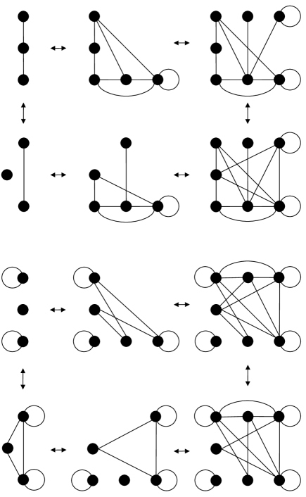
Figure 13: All of the $\Omega.3$ moves for marked graphs are inter-related through composition with $\Omega.2$ moves.

4 The extended marked-graph bracket

Suppose $U$ is any 4-regular graph, with $\phi$ free loops and $c(U)$ connected components. A circuit in $U$ is a sequence $v_{1}$, $h_{1}$, $h_{1}^{\prime}$, $v_{2}$, …, $v_{k}$, $h_{k}$, $h_{k}^{\prime}$, $v_{k+1}=v_{1}$ such that for each $i$, $h_{i}$ and $h_{i}^{\prime}$ are the half-edges of an edge $e_{i}$ connecting $v_{i}$ to $v_{i+1}$. (It is technically necessary to refer to half-edges because a loop is regarded as providing two different one-edge circuits, with opposite orientations.) There are $3^{n}$ partitions of $E(G)$ into circuits, each of which is determined by choosing one of the three transitions (pairings of incident half-edges) at every vertex. Each circuit partition is also required to include all the free loops of $U$. Let $C$ be an Euler system for $U$; choose one of the two orientations for each circuit that appears in $U$, and let $\vec{U}$ be the 2-in, 2-out digraph obtained from $U$ by using these orientations to assign directions to edges. Then as indicated in Fig. 14, the three transitions at a vertex $v$ are identified by their relationships with $C$: one follows $C$, one is consistent with the edge-directions of $\vec{U}$ without following $C$, and the third is inconsistent with the edge-directions of $\vec{U}$. Note that changing the choice of orientations for the elements of $C$ does not affect these designations.

The tool that allows us to use interlacement to describe the Kauffman bracket is the circuit-nullity formula. This formula has a very interesting history; at least five different special cases have been discovered during the last century [4, 6, 7, 25, 31, 38]. We refer to [33] for a detailed exposition, and only summarize the basic idea here. The three transitions pictured in Fig. 14 are represented (respectively) by three operations on the simple interlacement graph of $\vec{U}$ with respect to $C$: delete $v$, do nothing to $v$, and attach a loop at $v$. If $P$ is a circuit partition of $U$ then the circuit-nullity formula states that the number of elements of $P$ is

$$\left|P\right|=c(U)+\nu(\mathcal{A}_{P}),$$

where $\nu(\mathcal{A}_{P})$ is the $GF(2)$-nullity of the adjacency matrix of the graph obtained from the interlacement graph of $\vec{U}$ with respect to $C$ by performing, at each vertex, the operation corresponding to the transition used in $P$.

Figure 14: The three transitions at a vertex, in relation to an oriented Euler circuit: one transition follows the circuit, the second is consistent with the edge-directions determined by the Euler circuit, and the third is not consistent with these edge-directions.

Looking at Figs. 6 and 14, we see that if $U$ is the universe of a link diagram $D$ then vertex marks determine which transitions correspond to the $A$ and $B$ smoothings at a positive crossing as in Table 1. The transitions corresponding to the $A$ and $B$ smoothings at a negative crossing are simply interchanged.

vertex mark $$A$$ transition transition

(unmarked) orientation-consistent orientation-inconsistent

orientation-inconsistent orientation-consistent

follow orientation-inconsistent

orientation-inconsistent follow

orientation-consistent follow

follow orientation-consistent

(1)

These considerations motivate the following definitions.

Definition 15

Let $G$ be a graph with $V(G)=\{v_{1}$, $...$, $v_{n}\}$. The Boolean adjacency matrix of $G$ is the $n\times n$ matrix $\mathcal{A}(G)$ with entries in $GF(2)$ defined by: if $i\neq j$ then $\mathcal{A}(G)_{ij}=1$ if and only if $v_{i}$ is adjacent to $v_{j}$, and $\mathcal{A}(G)_{ii}=1$ if and only if $v_{i}$ is looped.

Observe that $\mathcal{A}(G)$ is defined if $G$ has multiple edges or multiple loops, but they do not affect it.

Definition 16

Let $G$ be a marked graph with $V(G)=\{v_{1}$, $...$, $v_{n}\}$. Suppose $T\subseteq V(G)$, and let $\Delta_{T}$ be the $n\times n$ matrix with the following entries in $GF(2)$.

$$(\Delta_{T})_{ij}=\left\{\begin{tabular}[c]{ll}$0,$&if $i\neq j$\\ $1,$&if $i=j$ and $v_{i}\in T$ has a mark with no $r$\\ $0,$&if $i=j$ and $v_{i}\in T$ has a mark with an $r$\\ $1,$&if $i=j$ and $v_{i}\not\in T$ has a mark with an $r$\\ $0,$&if $i=j$ and $v_{i}\not\in T$ has a mark with no $r$\end{tabular}\right.$$

Then $\mathcal{A}(G)_{T}$ is defined to be the submatrix of $\mathcal{A}(G)+\Delta_{T}$ obtained by removing the $i^{th}$ row and column if either (a) $v_{i}$ is marked $c$ or $cr$ and $(\mathcal{A}(G)+\Delta_{T})_{ii}=0$ or (b) $v_{i}$ is marked $u$ or $ur$ and $(\mathcal{A}(G)+\Delta_{T})_{ii}=1$.

Definition 17

The marked-graph bracket polynomial of a marked graph $G$ with $\phi$ free loops and $V(G)=\{v_{1}$, $...$, $v_{n}\}$ is

$$[G]=d^{\phi}\cdot\sum_{T\subseteq V(G)}A^{n-\left|T\right|}B^{\left|T\right|}d^{\nu(\mathcal{A}(G)_{T})},$$

where $\nu(\mathcal{A}(G)_{T})$ is the $GF(2)$-nullity of $\mathcal{A}(G)_{T}$.

Although the definition of $[G]$ requires an ordering of $V(G)$, choosing one ordering rather than another simply permutes the rows and columns of $\mathcal{A}(G)$; obviously this does not affect $[G]$. The next two results are almost as obvious.

Proposition 18

If $G^{\prime}$ is obtained from $G$ by toggling both the loop status and the letter $r$ in the mark of a vertex $v$, then $[G]=[G^{\prime}]$.

Proof. Table 1 indicates that toggling the letter $r$ in the mark of $v$ has the same effect on the bracket as toggling the loop status of $v$: the $A$ and $B$ transitions at $v$ are interchanged. Consequently, toggling both the loop status and the letter $r$ has no effect at all.   

Theorem 19

If $D$ is a virtual link diagram then $[\mathcal{L}(D$, $C)]$ is the same as the Kauffman bracket $[D]$.

Proof. For each subset $T\subseteq V(\mathcal{L}(D$, $C))$ let $S(T)$ be the Kauffman state of $D$ that involves $B$ smoothings at the vertices of $T$ and $A$ smoothings elsewhere. The number of closed curves in $S(T)$ is related to the binary nullity of $\mathcal{A}(G)_{T}$ by the circuit-nullity equality: $c(S(T))=c(U)+\nu(\mathcal{A}(G)_{T})$. As $\mathcal{L}(D$, $C)$ has $\phi=c(U)-1$ free loops, the theorem follows immediately.   

It follows that $[\mathcal{L}(D,C)]$ is not affected by the choice of $C$. According to Theorem 7, this is equivalent to saying that $[\mathcal{L}(D,C)]$ is invariant under marked local complementation. This invariance actually holds for arbitrary marked graphs, not just those that arise from link diagrams.

Theorem 20

If $G$ is a marked graph then $[G]=[G_{cru}^{v}]$ for every $v\in V(G)$.

Indeed, Theorem 20 is true term by term; that is, each subset $T\subseteq V(G)$ makes the same contribution to $[G]$ and $[G_{cru}^{v}]$.

Theorem 21

Let $G$ be a marked graph with a vertex $v$. Then for every subset $T\subseteq V(G)$,

$$\nu(\mathcal{A}(G)_{T})=\nu(\mathcal{A}(G_{cru}^{v})_{T}).$$

Proof. Let $V(G)=\{v_{1},...,v_{n}\}$, with $v=v_{1}$. Let $\Delta_{T}=\Delta_{T}(G)$ and $\Delta_{T}^{\prime}=\Delta_{T}(G_{cru}^{v})$ be the diagonal matrices that appear in Definition 16; they differ in the diagonal entries corresponding to neighbors of $v$, and also in the diagonal entry corresponding to $v$ if the mark of $v$ is $c$ or $cr$.

Suppose $i\geq 2$. We claim that Definition 16 tells us to remove the $i^{th}$ row and column of $\mathcal{A}(G)+\Delta_{T}$ in constructing $\mathcal{A}(G)_{T}$ if and only if it tells us to remove the $i^{th}$ row and column of $\mathcal{A}(G_{cru}^{v})+\Delta_{T}^{\prime}$ in constructing $\mathcal{A}(G_{cru}^{v})_{T}$. If $v_{i}$ is not a neighbor of $v$, then $v_{i}$ has the same mark in $G_{cru}^{v}$ as in $G$, and $(\mathcal{A}(G)+\Delta_{T})_{ii}=(\mathcal{A}(G_{cru}^{v})+\Delta_{T}^{\prime})_{ii}$, so the claim is satisfied. If $v_{i}$ is a neighbor of $v$ marked $c$ or $u$ in $G$, then $v_{i}$ is marked $ur$ or $cr$ (respectively) in $G_{cru}^{v}$; moreover, $(\mathcal{A}(G)+\Delta_{T})_{ii}\neq(\mathcal{A}(G_{cru}^{v})+\Delta_{T}^{\prime})_{ii}$ because $(\Delta_{T})_{ii}\neq(\Delta_{T}^{\prime})_{ii}$. Consequently the claim is satisfied. Similarly, the claim is satisfied if $v_{i}$ is a neighbor of $v$ marked $cr$ or $ur$. Finally, if $v_{i}$ is a neighbor of $v$ that is unmarked or marked $r$ in $G$ then $v_{i}$ is marked $r$ or unmarked (respectively) in $G_{cru}^{v}$; either way Definition 16 does not tell us to remove the $i^{th}$ row and column of $\mathcal{A}(G)+\Delta_{T}$ or $\mathcal{A}(G_{cru}^{v})+\Delta_{T}^{\prime}$. This completes the proof of the claim.

If $(\mathcal{A}(G)+\Delta_{T})_{11}=0$ and $v$ is not marked $c$ or $cr$ in $G$, then the same is true in $G_{cru}^{v}$ and we verify that

$$\nu(\mathcal{A}(G)_{T})=\nu\begin{pmatrix}0&\mathbf{1}&\mathbf{0}\\ \mathbf{1}&M_{11}&M_{12}\\ \mathbf{0}&M_{21}&M_{22}\end{pmatrix}=\nu\begin{pmatrix}0&\mathbf{1}&\mathbf{0}\\ \mathbf{1}&\bar{M}_{11}&M_{12}\\ \mathbf{0}&M_{21}&M_{22}\end{pmatrix}=\nu(\mathcal{A}(G_{cru}^{v})_{T})$$

by adding the top row to every row in the second set of rows. (Bold numerals denote rows and columns whose entries are all the same, and $\bar{M}_{11}$ denotes the matrix obtained by toggling every entry of $M_{11}$.)

If $(\mathcal{A}(G)+\Delta_{T})_{11}=0$ and $v$ is marked $c$ or $cr$ in $G$, then $(\mathcal{A}(G_{cru}^{v})+\Delta_{T}^{\prime})_{11}=1$ and $v$ is marked $cr$ or $c$ (respectively) in $G_{cru}^{v}$, so

$$\nu\begin{pmatrix}M_{11}&M_{12}\\ M_{21}&M_{22}\end{pmatrix}=\nu\begin{pmatrix}1&\mathbf{1}&\mathbf{0}\\ \mathbf{0}&M_{11}&M_{12}\\ \mathbf{0}&M_{21}&M_{22}\end{pmatrix}=\nu\begin{pmatrix}1&\mathbf{1}&\mathbf{0}\\ \mathbf{1}&\bar{M}_{11}&M_{12}\\ \mathbf{0}&M_{21}&M_{22}\end{pmatrix}$$

verifies that $\nu(\mathcal{A}(G)_{T})=\nu(\mathcal{A}(G_{cru}^{v})_{T})$. The same calculation applies if $(\mathcal{A}(G)+\Delta_{T})_{11}=1$ and $v$ is marked $u$ or $ur$ in $G$.

If $(\mathcal{A}(G)+\Delta_{T})_{11}=1$ and $v$ is not marked $u$ or $ur$ in $G$, a similar calculation shows that $\nu(\mathcal{A}(G)_{T})=\nu(\mathcal{A}(G_{cru}^{v})_{T})$.

$$\nu\begin{pmatrix}1&\mathbf{1}&\mathbf{0}\\ \mathbf{1}&M_{11}&M_{12}\\ \mathbf{0}&M_{21}&M_{22}\end{pmatrix}=\nu\begin{pmatrix}1&\mathbf{1}&\mathbf{0}\\ \mathbf{0}&\bar{M}_{11}&M_{12}\\ \mathbf{0}&M_{21}&M_{22}\end{pmatrix}=\nu\begin{pmatrix}\bar{M}_{11}&M_{12}\\ M_{21}&M_{22}\end{pmatrix}.$$

 

With Theorems 19 and 20 in hand, we conclude that Kauffman’s classical construction of the Jones polynomial from the bracket [18] extends directly to multiply marked graphs.

Definition 22

The reduced marked-graph bracket polynomial $\left\langle G\right\rangle$ is the image of the three-variable marked-graph bracket under the evaluations $B\mapsto A^{-1}$ and $d\mapsto-A^{-2}-A^{2}$.

Definition 23

The marked-graph Jones polynomial of a graph with $\ell$ looped vertices and $n-\ell$ unlooped vertices is

$$V_{G}(t)=(-1)^{n}\cdot t^{(3n-6\ell)/4}\cdot\left\langle G\right\rangle(t^{-1/4}).$$

Theorem 24

The reduced bracket is invariant under marked local complementations and marked-graph Reidemeister moves of types $\Omega.2$ and $\Omega.3$. The marked-graph Jones polynomial is invariant under marked local complementations and all three types of marked-graph Reidemeister moves.

Proof. The invariance of $\left\langle G\right\rangle$ under marked local complementations follows from Theorem 20, and the invariance of $\left\langle G\right\rangle$ under $\Omega.2$ and $\Omega.3$ moves is proven using the same matrix-nullity arguments that appear in [34]. The invariance of the Jones polynomial follows from the fact that the effects of an $\Omega.1$ move on $(-1)^{n}\cdot t^{(3n-6\ell)/4}$ and $\left\langle G\right\rangle(t^{-1/4})$ cancel each other.   

5 Some equivalence relations

In this section we briefly discuss several equivalence relations that come to mind when we consider links and marked graphs.

1. The finest interesting equivalence relation on marked graphs is generated by the marked pivots of Definition 9. As proved in [34], results of Kotzig [21], Pevzner [27] and Ukkonen [37] imply that if $D$ is an oriented link diagram and $C$ is any directed Euler system of $D$ then the equivalence class of $\mathcal{L}(D,C)$ is the set of interlacement graphs $\mathcal{L}(D,C^{\prime})$ corresponding to various directed Euler systems $C^{\prime}$ of $D$.

2. A strictly coarser equivalence relation on marked graphs is generated by marked local complementation. Theorem 7 tells us that this relation extends the relation tying $\mathcal{L}(D$, $C)$ to $\mathcal{L}(D$, $C^{\prime})$ for arbitrary Euler systems $C$ and $C^{\prime}$ in an oriented link diagram $D$, i.e. if $\mathcal{G}_{cru}$ denotes the set of equivalence classes of multiply marked graphs under this relation and $\mathcal{D}$ denotes the set of oriented link diagrams then the marked interlacement graph construction provides a well-defined function $\mathcal{L}:\mathcal{D}\rightarrow\mathcal{G}_{cru}$. Two singly marked graphs that arise from link diagrams are equivalent under this relation if and only if they are equivalent under the first relation; we do not know whether or not this property extends to arbitrary singly marked graphs. Theorem 20 tells us that the bracket $[~{}]$ is well-defined on $\mathcal{G}_{cru}$, and Theorem 19 tells us that the Kauffman bracket is defined on $\mathcal{D}$ by the composition $[~{}]\circ\mathcal{L}$.

3. Reidemeister equivalence is the equivalence relation $\sim$ on marked graphs generated by marked-graph Reidemeister moves and marked local complementation. Theorem 14 tells us that this relation extends the relation tying $\mathcal{L}(D$, $C)$ to $\mathcal{L}(D^{\prime}$, $C^{\prime})$ for arbitrary Euler systems $C$ and $C^{\prime}$ in diagrams $D$ and $D^{\prime}$ representing the same virtual link type. That is, if $\sim$ denotes the link type equivalence relation on $\mathcal{D}$ then $\mathcal{L}:\mathcal{D}\rightarrow\mathcal{G}_{cru}$ induces a well-defined function ${\widetilde{\mathcal{L}}}:\mathcal{D}/\!\sim~{}\rightarrow~{}\mathcal{G}_{cru}/\!\sim$. The marked-graph Jones polynomial is a well-defined function on $\mathcal{G}_{cru}/\!\sim$, whose composition with ${\widetilde{\mathcal{L}}}$ is the familiar Jones polynomial of virtual links.

4. Regular isotopy is the finer equivalence relation that does not involve $\Omega.1$ moves. The reduced bracket and the writhe are well-defined modulo regular isotopy.

5. There are several equivalence relations on link diagrams that are connected to the functions $\mathcal{L}$ and ${\widetilde{\mathcal{L}}}$. For instance, suppose $D$ and $D^{\prime}$ are link diagrams and there is an isomorphism between the oriented universe graphs $\vec{U}$ and $\overrightarrow{U^{\prime}}$ that maps the directed circuits corresponding to the link components in $D$ to the directed circuits corresponding to the link components in $D^{\prime}$. Then $\mathcal{L}$ cannot distinguish between $D$ and $D^{\prime}$. If $D_{1}$ and $D_{2}$ are diagrams then $\mathcal{L}$ cannot distinguish between different connected sums $D_{1}\#D_{2}$, or between a split union $D_{1}\cup D_{2}$ and a diagram obtained by adding a free loop to a connected sum $D_{1}\#D_{2}$.

6. Every marked graph $G$ has an $r$-simplification $G_{r}$ obtained by removing the $r$ from every vertex of $G$ whose mark includes one, and toggling the loop status of each such vertex. Proposition 18 tells us that $[G]=[G_{r}]$, so when discussing $[G]$ it is reasonable to consider the equivalence relation generated by local complementation and $r$-simplification, and when discussing $\left\langle G\right\rangle$ it is reasonable to consider the equivalence relation generated by regular isotopy and $r$-simplification.

The first versions of this paper incorporated $r$-simplification throughout. However, in link diagrams the loop status and the $r$ status of a crossing reflect different kinds of information: the loop status reflects the sign of the crossing, and the $r$ status reflects the way an Euler circuit traverses the crossing. Consequently $r$-simplification involves the loss of valuable information about link diagrams. For example, Fig. 15 shows that even though $\mathcal{L}(D,C)$ determines both the writhe and the Jones polynomial, $\mathcal{L}(D,C)_{r}$ determines neither. (In any diagram of a multi-component link, reversing the orientation of one link component will have the same effect: every crossing involving that link component and another will have both its loop status and its $r$ status toggled.)

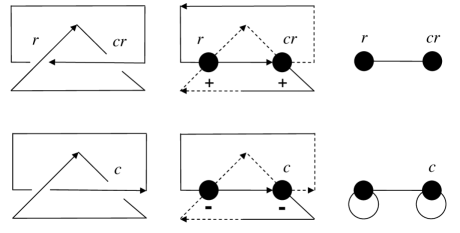
Figure 15: Diagrams of the positive and negative Hopf link have associated interlacement graphs whose $r$-simplifications are isomorphic.

6 Graph-links

Definition 25

[15] A labeled graph $G$ is a simple graph each of whose vertices is labeled by a pair $(a$, $\alpha)\in\{0$, $1\}\times\{+$, $-\}$.

Definition 26

[15] A graph-link is an equivalence class of labeled graphs under the equivalence relation generated by the following operations.

$\Omega_{g}1$. Adjoin or remove an isolated vertex with label $(0$, $\pm)$.

$\Omega_{g}2$. Adjoin or remove a pair of non-adjacent (resp. adjacent) vertices that are labeled $(0$, $\pm\alpha)$ (resp. $(1$, $\pm\alpha)$) and have the same adjacencies with other vertices.

$\Omega_{g}3$. Suppose $G$ has three distinct vertices $v$, $w$, $x$ labeled $(0$, $-)$, such that the only neighbors of $x$ are $v$ and $w$, which are not neighbors of each other. Then change the labels of $v$ and $w$ to $(0$, $+)$, make $x$ adjacent to every vertex that is adjacent to precisely one of $v$, $w$, and remove the edges connecting $x$ to $v$ and $w$. (The inverse of this operation is also an $\Omega_{g}3$ move.)

$\Omega_{g}4$. Suppose $G$ has two adjacent vertices $v$ and $w$ labeled $(0$, $\alpha)$ and $(0$, $\beta)$. Replace $G$ with $((G^{v})^{w})^{v}$ and then change the labels of $v$ and $w$ to $(0$, $-\beta)$ and $(0$, $-\alpha)$ respectively. (The inverse is also an $\Omega_{g}4$ move.)

$\Omega_{g}4^{\prime}$. Suppose $G$ has a vertex $v$ with label $(1$, $\alpha)$. Replace $G$ with $G^{v}$, change the label of $v$ to $(1$, $-\alpha)$, and change the label of each neighbor of $v$ by changing the first coordinate and leaving the second coordinate the same. (The inverse is also an $\Omega_{g}4^{\prime}$ move.)

Definition 27

The marked graph $mark(G)$ associated to a labeled graph $G$ is obtained by preserving all non-loop edges and changing labels to loop-mark combinations as follows: $(0$, $+)$ becomes $u$ with a loop; $(0$, $-)$ becomes $u$ with no loop; $(1$, $+)$ becomes $c$ with no loop; and $(1$, $-)$ becomes $c$ with a loop.

The fact that the vertex marks in $mark(G)$ do not involve the letter $r$ indicates that the relationship between marked graphs and graph-links involves the notion of $r$-simplification mentioned in Section 5.

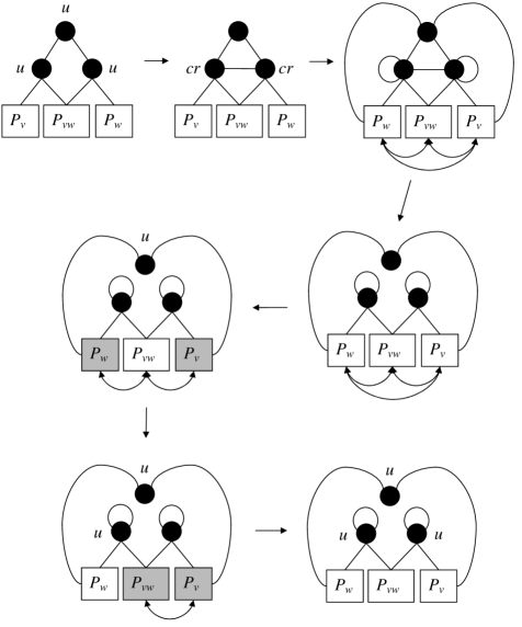
Figure 16: The marked-graph version of the graph-link $\Omega_{g}3$ move is a composition of $r$-simplifications with a marked local complementation, a marked pivot, one of the $\Omega.3$ moves of Figure 12, and three marked local complementations.

Theorem 28

If two labeled graphs $G$ and $H$ define the same graph-link then the corresponding marked graphs $mark(G)$ and $mark(H)$ are equivalent under marked local complementation, $r$-simplification and marked-graph Reidemeister moves.

Proof. An $\Omega_{g}4^{\prime}$ move corresponds to the $r$-simplification of a marked local complementation at $v$, and an $\Omega_{g}4$ move corresponds to the $r$-simplification of a marked pivot with respect to $v$ and $w$.

The first three types of graph-link operations correspond to marked-graph Reidemeister moves. An $\Omega_{g}1$ move corresponds to a marked-graph $\Omega.1$ move. An $\Omega_{g}2$ move performed on vertices labeled $(0$, $\pm\alpha)$ corresponds to an instance of Definition 11 (b) in the $r$-simplification of $(G_{cru}^{v})_{cru}^{w}$. An $\Omega_{g}2$ move performed on vertices labeled $(1$, $\pm\alpha)$, on the other hand, corresponds to an instance of Definition 11 (a) in the $r$-simplification of $G_{cru}^{vw}$.

The $\Omega_{g}3$ moves are more complicated. Let $P_{v}$, $P_{w}$, $P_{vw}\subseteq V(G)-\{v$, $w$, $x\}$ consist of those vertices that are adjacent to $v$ and not $w$, $w$ and not $v$, and both $v$ and $w$ (respectively). Also, let $H$ be the labeled graph that results from the $\Omega_{g}3$ move. Let $G^{\prime}$ be the marked graph obtained from $mark(G)$ by performing a marked local complementation at $x$, a marked pivot with respect to $v$ and $w$, and then an $r$-simplification. Then $v$, $w$ and $x$ are all unmarked in $G^{\prime}$, and they induce a subgraph isomorphic to the third one pictured in Fig. 12, with $x$ unlooped. According to Lemma 8, the neighbors of $v$ in $G^{\prime}$ are the elements of $P_{vw}\cup P_{w}$, the neighbors of $w$ in $G^{\prime}$ are the elements of $P_{v}\cup P_{vw}$, and the neighbors of $x$ in $G^{\prime}$ are the elements of $P_{v}\cup P_{w}$. An $\Omega.3$ move performed on this subgraph of $G^{\prime}$ results in a graph $G^{\prime\prime}$ that resembles $mark(H)$ in that no two of $v$, $w$, $x$ are neighbors, $v$ and $w$ are looped, and $x$ is not looped. However $v$, $w$ and $x$ are all unmarked, while in $mark(H)$ they are all marked $u$; also the adjacencies among their neighbors do not match those of $mark(H)$, because of the toggling of adjacencies between vertices from different elements of $\{P_{v}$, $P_{w}$, $P_{vw}\}$. Both problems are solved by applying $r$-simplifications and marked local complementations at $x$, $v$ and $w$. (The marked pivot in the second step exchanges the neighbors of $v$ and $w$, but of course this is insignificant up to isomorphism.)

This process is pictured in Fig. 16. At the top left of the figure we see $mark(G)$; the vertices $v$, $w$, $x$ are not named in the figure but they are determined by their neighborhoods. Moving from left to right along the top row we see the result of applying a marked local complementation at $x$,  and then a marked pivot with respect to $v$ and $w$ followed by an $r$-simplification. (The double-headed arrows indicate the toggling of adjacencies between vertices in different elements of $\{P_{v}$, $P_{w}$, $P_{vw}\}$.) After applying an $\Omega.3$ move we obtain $G^{\prime\prime}$, the graph pictured on the right in the second row of the figure. The graph pictured to the left of $G^{\prime\prime}$ is $((G^{\prime\prime})_{cru}^{x})_{r}$; the gray boxes indicate the toggling of loops and non-loop edges within $P_{w}$ and $P_{v}$. The last two graphs are obtained by marked local complementations first at $v$ and then at $w$, followed by $r$-simplifications.   

Theorem 28 does not completely describe the relationship between graph-links and marked graphs. On the one hand, some of the marked-graph local complementation and Reidemeister moves do not occur among the graph-link Reidemeister moves. For instance there is no need for $\Omega_{g}4^{\prime}$ moves at vertices with labels $(0,\alpha)$, because the corresponding $\kappa$-transformations would not produce rotating circuits. This difference may allow some labeled graphs $G$ and $H$ to define inequivalent graph-links even if $mark(G)$ and $mark(H)$ are equivalent under Reidemeister moves and $r$-simplification. On the other hand, the fact that equivalence of graph-links is associated with $r$-simplification raises the possibility that there may be labeled graphs $G$ and $H$ that define the same graph-link, but whose associated marked graphs are not Reidemeister equivalent.

7 Recursion

We begin developing the recursion of Theorem 1 by discussing the relationships among the bracket polynomials of graphs that differ only in the loop-mark combination at a single vertex $v$. Denote a graph obtained from $G$ by changing only the loop-mark combination at $v$ by $G(v,x)$, where $x$ tells us how $v$ has been changed: in $G(v,c,\ell)$ the vertex $v$ is marked $c$ and looped, in $G(v,ur)$ the vertex $v$ is marked $ur$ and unlooped, in $G(v,\ell)$ the vertex $v$ is unmarked and looped, in $G(v)$ the vertex $v$ is unmarked and unlooped, and so on. Observe that the notations $G-v$ and $G_{cru}^{v}-v$ are unambiguous, because these graphs are not affected if we change the loop-mark status of $v$.

Split $[G(v)]$ into two separate sums as follows:

$$S =d^{\phi}\cdot\sum_{v\not\in T\subseteq V(G)}A^{n-\left|T\right|}B^{\left|T\right|}d^{\nu(\mathcal{A}(G(v))_{T})}\text{ }$$

$$\text{and }S^{\prime} =d^{\phi}\cdot\sum_{v\in T\subseteq V(G)}A^{n-\left|T\right|}B^{\left|T\right|}d^{\nu(\mathcal{A}(G(v))_{T})}.$$

We claim that $S^{\prime}=B[G_{cru}^{v}-v]$. If $v\in T\subseteq V(G(v))=V(G(v)_{cru}^{v})$ then Theorem 21 tells us that $\nu(\mathcal{A}(G(v))_{T})=\nu(\mathcal{A}(G(v)_{cru}^{v})_{T})$, and Definition 6 tells us that as $v$ is unlooped and unmarked in $G(v)$, it is unlooped and marked $u$ in $G(v)_{cru}^{v}$. Definition 16 then tells us that the row and column of $\mathcal{A}(G(v)_{cru}^{v})+\Delta_{T}$ corresponding to $v$ are deleted in obtaining $\mathcal{A}(G(v)_{cru}^{v})_{T}$; it follows that $\mathcal{A}(G(v)_{cru}^{v})_{T}=\mathcal{A}(G_{cru}^{v}-v)_{T-\{v\}}$, and consequently $\nu(\mathcal{A}(G_{cru}^{v}-v)_{T-\{v\}})=\nu(\mathcal{A}(G(v)_{cru}^{v})_{T})=\nu(\mathcal{A}(G(v))_{T})$. Summing over $T$ yields $B[G_{cru}^{v}-v]=S^{\prime}$.

Definitions 16 and 17 tell us that changing the mark of $v$ to $r$ has the same effect as toggling between $v\in T$ and $v\notin T$; hence $[G(v,r)]=A^{-1}BS+B^{-1}AS^{\prime}=A^{-1}BS+A[G_{cru}^{v}-v]$.

Now split $[G(v,u)]$ into two separate sums as follows:

$$S =d^{\phi}\cdot\sum_{v\not\in T\subseteq V(G)}A^{n-\left|T\right|}B^{\left|T\right|}d^{\nu(\mathcal{A}(G(v,u))_{T})}\text{ }$$

$$\text{and }S^{\prime\prime} =d^{\phi}\cdot\sum_{v\in T\subseteq V(G)}A^{n-\left|T\right|}B^{\left|T\right|}d^{\nu(\mathcal{A}(G(v,u))_{T})}.$$

Definition 16 tells us that $\mathcal{A}(G(v))_{T}=\mathcal{A}(G(v,u))_{T}$ if $v\notin T$, so this $S$ is the same as the sum denoted $S$ in the above analysis of $[G(v)]$. Definition 16 also tells us that $\mathcal{A}(G(v,u))_{T}=\mathcal{A}(G-v)_{T-\{v\}}$ if $v\in T$; summing over these $T$ we see that $S^{\prime\prime}=B[G-v]$.

Definitions 16 and 17 imply that $[G(v,ur)]=A^{-1}BS+B^{-1}AS^{\prime\prime}=A^{-1}BS+A[G-v]$.

Finally, observe that Definition 16 implies $\mathcal{A}(G(v,c))_{T}=\mathcal{A}(G(v))_{T}$ if $v\in T$ and $\mathcal{A}(G(v,c))_{T}=\mathcal{A}(G(v,u))_{T\cup\{v\}}$ if $v\not\in T$. Consequently $[G(v,c)]=S^{\prime}+AB^{-1}S^{\prime\prime}=$ $B[G_{cru}^{v}-v]+A[G-v]$. Changing the mark of $v$ to $cr$ reverses the coefficients: $[G(v,cr)]=A[G_{cru}^{v}-v]+B[G-v]$.

In sum, we have the following equalities:

$$[G(v)] =S+B[G_{cru}^{v}-v]$$ (7.1)

$$[G(v,r)] =A^{-1}BS+A[G_{cru}^{v}-v]$$

$$[G(v,c)] =A[G-v]+B[G_{cru}^{v}-v]$$

$$[G(v,cr)] =B[G-v]+A[G_{cru}^{v}-v]$$

$$[G(v,u)] =S+B[G-v]$$

$$[G(v,ur)] =A^{-1}BS+A[G-v]$$

Recall that Proposition 18 tells us that $[G(v,\ell)]=[G(v,r)]$, $[G(v,ur,\ell)]=[G(v,u)]$ and so on. Note also that in case $D$ is a link diagram with $G=\mathcal{L}(D,C)$, the six equalities of (7.1) correspond to the six different ways the Euler system $C$ might be related to the $A$ and $B$ smoothings at the crossing of $D$ corresponding to $v$; see Fig. 6.

The proof of Theorem 1 is now very simple. Parts (a) – (c) follow from Definition 17, parts (e) and (f) follow from Theorem 20, and part (d) follows from Proposition 18 and the formulas for $[G(v,c)]$ and $[G(v,cr)]$ in (7.1). To perform a computation, first use (a) – (d) to remove free loops, isolated vertices and vertices marked $c$ or $cr$. Suppose a nonempty graph has no vertex marked $c$ or $cr$, and no isolated vertex. If $v$ has a neighbor marked $u$ or $ur$ then in $G_{cru}^{v}$ every such neighbor is marked $c$ or $cr$, and can be removed with (d). If there is no vertex with a neighbor marked $u$ or $ur$ then there are two neighbors $v$ and $w$ each of which is either unmarked or marked $r$; $w$ is marked $u$ or $ur$ in $G_{cru}^{w}$, so (e) may be applied to $v$ in $G_{cru}^{w}$.

If we compare Theorem 1 to the recursions discussed in [34, 35, 36], we see that two recursive steps have been removed in favor of marked local complementations. The marked local complementations are preferable because they do not involve replacing one graph with two or three graphs, but the old recursive steps are still valid.

Proposition 29

If $v\in V(G)$ is looped and unmarked then

$$[G]=A^{-1}B[G-\{v,v\}]+(A-A^{-1}B^{2})[G_{cru}^{v}-v]\text{, }$$

where $G-\{v,v\}$ is obtained from $G$ by removing the loop at $v$. Also, if $v$ and $w$ are two unlooped, unmarked neighbors in $G$ then

$$[G]=A^{2}[G_{cru}^{vw}-v-w]+AB[(G_{cru}^{w})_{cru}^{v}-v-w]+B[G_{cru}^{v}-v].$$

Proof. The first part follows immediately from the formulas (7.1).

Suppose $v\neq w\in V(G)$ are adjacent, unlooped, and unmarked. Let

$$S_{00}=\sum_{\begin{subarray}{c}T\subseteq V(G)\\ v\notin T,w\notin T\end{subarray}}A^{n-\left|T\right|}B^{\left|T\right|}d^{\nu(\mathcal{A}(G)_{T})}\text{, }S_{01}=\sum_{\begin{subarray}{c}T\subseteq V(G)\\ v\notin T,w\in T\end{subarray}}A^{n-\left|T\right|}B^{\left|T\right|}d^{\nu(\mathcal{A}(G)_{T})}$$

$$\text{and }S_{1}=\sum_{\begin{subarray}{c}T\subseteq V(G)\\ v\in T\end{subarray}}A^{n-\left|T\right|}B^{\left|T\right|}d^{\nu(\mathcal{A}(G)_{T})}\text{ .}$$

As discussed in the second paragraph of this section, $S_{1}=B[G_{cru}^{v}-v]$.

Suppose $v,w\notin$ $T\subseteq V(G)$. Theorem 21 tells us $\nu(\mathcal{A}(G)_{T})=\nu(\mathcal{A}(G_{cru}^{vw})_{T})$. As $v$ and $w$ are both unmarked in $G$, Lemma 8 and Definition 9 tell us that $v$ and $w$ are both marked $c$ in $G_{cru}^{vw}$. As they are both unlooped and not in $T$, the definition of $\mathcal{A}(G_{cru}^{vw})_{T}$ involves deleting the rows and columns of $\mathcal{A}(G_{cru}^{vw})+\Delta_{T}$ corresponding to both $v$ and $w$. Consequently $\mathcal{A}(G_{cru}^{vw})_{T}=\mathcal{A}(G_{cru}^{vw}-v-w)_{T}$. Summing over $T$, we see that

$$S_{00}=A^{2}[G_{cru}^{vw}-v-w].$$

Suppose $v\notin T\subseteq V(G)$ and $w\in T$. Theorem 21 tells us that $\nu(\mathcal{A}(G)_{T})=\nu(\mathcal{A}((G_{cru}^{w})_{cru}^{v})_{T})$. In $G$, $v$ and $w$ are both unlooped and unmarked; in $G_{cru}^{w}$, $w$ is unlooped and marked $u$ and $v$ is unlooped and marked $r$; and in $(G_{cru}^{w})_{cru}^{v}$, $v$ is unlooped and marked $ur$ and $w$ is unlooped and marked $cr$. As $v\notin T$ and $w\in T$, the definition of $\mathcal{A}((G_{cru}^{w})_{cru}^{v})_{T}$ involves deleting the rows and columns of $\mathcal{A}((G_{cru}^{w})_{cru}^{v})+\Delta_{T}$ corresponding to $v$ and $w$; summing over $T$ yields

$$S_{01}=AB[(G_{cru}^{w})_{cru}^{v}-v-w].$$

$[G]=S_{1}+S_{00}+S_{01}$, so the second equality of the proposition follows.   

As noted in [34] and [36], for link diagrams the formulas of Proposition 29 correspond to well-known properties of the Kauffman bracket. The first corresponds to the Kauffman bracket’s switching formula (denoted $A\chi-A^{-1}\bar{\chi}=(A^{2}-A^{-2})\asymp$ in [20]), and the second corresponds to a double use of the basic recursion of the Kauffman bracket, $[D]=A^{2}[D_{AA}]+AB[D_{AB}]+B[D_{B}]$. The hypothesis “no neighbor of $v$ is marked” appeared when the formulas of Proposition 29 were used in [34] and [35], but this hypothesis was only necessary because we used ordinary (unmarked) local complementation there. The effect of the hypothesis is to restrict attention to situations in which the unmarked local complements are the same as $r$-simplifications of marked local complements.

8 Vertex weights

In [35] we discuss several advantages of extending the marked-graph bracket to graphs given with vertex weights, i.e. functions $\alpha$ and $\beta$ mapping $V(G)$ into some commutative ring $R$. The weighted form of the bracket is defined by using the weights in place of $A$ and $B$ in Definition 17:

$$[G]=d^{\phi}\cdot\sum_{T\subseteq V(G)}({\displaystyle\prod\limits_{v\notin T}}\alpha(v))({\displaystyle\prod\limits_{t\in T}}\beta(t)))d^{\nu(\mathcal{A}(G)_{T})}.$$

Theorem 21 tells us that if we extend marked local complementation to weighted graphs in the obvious way (i.e. local complementation does not affect vertex weights), then the weighted, marked-graph bracket polynomial is invariant under marked local complementations.

The simplest result of [35] is that reversing the $\alpha$ and $\beta$ weights of a vertex has the same effect as toggling its loop status. (The corresponding $A-B$ duality is apparent in the formulas of Section 7.) This observation may seem trivial but it is useful in simplifying recursive calculations that involve the first equality of Proposition 29: rather than replace a graph with two graphs each time we want to remove a loop, we simply interchange $\alpha(v)$ and $\beta(v)$ at each looped vertex. Similarly, if the mark of a vertex $v$ includes $r$ then $[G]$ is unchanged if we remove the $r$ and interchange $\alpha(v)$ and $\beta(v)$.

It is a simple matter to modify Theorem 1 to incorporate weights: just replace each occurrence of $A$ with $\alpha(v)$, and each occurrence of $B$ with $\beta(v)$.

There are also analogues of series-parallel reductions, involving twin vertices. (Recall from [35] that twin vertices occur naturally in the looped interlacement graphs of link diagrams: when two strands of a link are twisted around each other repeatedly, the resulting classical crossings correspond to twin vertices in $\mathcal{L}(D,C)$.) Some of these twin reductions are very much like series-parallel reductions; they replace several vertices with one re-weighted vertex in a single graph. Others are not completely analogous to series-parallel reductions as the reduced forms involve two different graphs. All are of some value in computation because they result in smaller graphs than part (d) of Theorem 1. There are several different cases; here are four.

Proposition 30

Let $v\neq w\in V(G)$ be nonadjacent, unlooped twin vertices. (That is, they have the same neighbors outside $\{v,w\}$.)

(a) Suppose that $v$ and $w$ are both marked $u$. Then $[G]=[(G-w)^{\prime}]$, where $(G-w)^{\prime}$ is obtained from $G-w$ by changing the weights of $v$ to $\alpha^{\prime}(v)=\alpha(v)\alpha(w)d+\alpha(v)\beta(w)+$ $\beta(v)\alpha(w)$ and $\beta^{\prime}(v)=\beta(v)\beta(w)$.

(b) Suppose that $v$ is unmarked and $w$ is marked $u$. Then $[G]=[(G-w)^{\prime}]\,$, where $(G-w)^{\prime}$ is obtained from $G-w$ by changing the weights of $v$ to $\alpha^{\prime}(v)=\alpha(v)\alpha(w)d+\alpha(v)\beta(w)+$ $\beta(v)\alpha(w)$ and $\beta^{\prime}(v)=\beta(v)\beta(w)$.

(c) Suppose that $v$ and $w$ are both unmarked. Then $[G]=[(G-w)^{\prime}]$, where $(G-w)^{\prime}$ is obtained from $G-w$ by giving $v$ a mark of $u$ and changing the weights of $v$ to $\alpha^{\prime}(v)=\alpha(v)\alpha(w)d+\alpha(v)\beta(w)+$ $\beta(v)\alpha(w)$ and $\beta^{\prime}(v)=\beta(v)\beta(w)$.

(d) Suppose that $v$ is marked $c$ and $w$ is marked $u$. Then $[G]=[(G-w)^{\prime}]+\alpha(v)\beta(w)[G-v-w]$, where $(G-w)^{\prime}$ is obtained from $G-w$ by unmarking $v$ and changing the weights of $v$ to $\alpha^{\prime}(v)=\alpha(v)\alpha(w)+$ $\beta(v)\alpha(w)$ and $\beta^{\prime}(v)=\beta(v)\beta(w)$.

Proof. (a) Suppose $V(G)=\{v_{1},...,v_{n}\}$ with $v=v_{1}$ and $w=v_{2}$. If $T\subseteq\{v_{3},...,v_{n}\}\,$ then the equality

$$\nu\begin{pmatrix}0&0&\mathbf{1}&\mathbf{0}\\ 0&0&\mathbf{1}&\mathbf{0}\\ \mathbf{1}&\mathbf{1}&M_{11}&M_{12}\\ \mathbf{0}&\mathbf{0}&M_{21}&M_{22}\end{pmatrix}-1=\nu\begin{pmatrix}0&\mathbf{1}&\mathbf{0}\\ \mathbf{1}&M_{11}&M_{12}\\ \mathbf{0}&M_{21}&M_{22}\end{pmatrix}$$

tells us that $\nu(\mathcal{A}(G)_{T})-1=\nu(\mathcal{A}((G-w)^{\prime})_{T})=\nu(\mathcal{A}(G)_{T\cup\{w\}})=\nu(\mathcal{A}(G)_{T\cup\{v\}})$. It follows that the contributions of $T$, $T\cup\{w\}$ and $T\cup\{v\}$ to $[G]$ sum to the contribution of $T$ to $[(G-w)^{\prime}]$. As

$$\mathcal{A}(G)_{T\cup\{v,w\}}=\begin{pmatrix}M_{11}&M_{12}\\ M_{21}&M_{22}\end{pmatrix}=\mathcal{A}((G-w)^{\prime})_{T\cup\{v\}},$$

the contribution of $T\cup\{v,w\}$ to $[G]$ coincides with the contribution of $T\cup\{v\}$ to $[(G-w)^{\prime}]$.

(b) If $T\subseteq\{v_{3},...,v_{n}\}\,$ then the equality

$$\nu\begin{pmatrix}0&0&\mathbf{1}&\mathbf{0}\\ 0&0&\mathbf{1}&\mathbf{0}\\ \mathbf{1}&\mathbf{1}&M_{11}&M_{12}\\ \mathbf{0}&\mathbf{0}&M_{21}&M_{22}\end{pmatrix}-1=\nu\begin{pmatrix}0&\mathbf{1}&\mathbf{0}\\ \mathbf{1}&M_{11}&M_{12}\\ \mathbf{0}&M_{21}&M_{22}\end{pmatrix}=\nu\begin{pmatrix}1&0&\mathbf{1}&\mathbf{0}\\ 0&0&\mathbf{1}&\mathbf{0}\\ \mathbf{1}&\mathbf{1}&M_{11}&M_{12}\\ \mathbf{0}&\mathbf{0}&M_{21}&M_{22}\end{pmatrix}$$

implies$\ \nu(\mathcal{A}(G)_{T})-1=\nu(\mathcal{A}((G-w)^{\prime})_{T})=\nu(\mathcal{A}(G)_{T\cup\{w\}})=\nu(\mathcal{A}(G)_{T\cup\{v\}})$. Also,

$$\mathcal{A}(G)_{T\cup\{v,w\}}=\begin{pmatrix}1&\mathbf{1}&\mathbf{0}\\ \mathbf{1}&M_{11}&M_{12}\\ \mathbf{0}&M_{21}&M_{22}\end{pmatrix}=\mathcal{A}((G-w)^{\prime})_{T\cup\{v\}}.$$

(c) The first equalities displayed for (b) still tell us that $\nu(\mathcal{A}(G)_{T})-1=\nu(\mathcal{A}((G-w)^{\prime})_{T})=\nu(\mathcal{A}(G)_{T\cup\{w\}})=\nu(\mathcal{A}(G)_{T\cup\{v\}})$. In this case $\mathcal{A}(G)_{T\cup\{v,w\}}\not=\mathcal{A(}(G-w)^{\prime})_{T\cup\{v\}}$ but $\nu(\mathcal{A}(G)_{T\cup\{v,w\}})=\nu(\mathcal{A(}(G-w)^{\prime})_{T\cup\{v\}})$ nevertheless, because

$$\nu\begin{pmatrix}1&0&\mathbf{1}&\mathbf{0}\\ 0&1&\mathbf{1}&\mathbf{0}\\ \mathbf{1}&\mathbf{1}&M_{11}&M_{12}\\ \mathbf{0}&\mathbf{0}&M_{21}&M_{22}\end{pmatrix}=\nu\begin{pmatrix}M_{11}&M_{12}\\ M_{21}&M_{22}\end{pmatrix}.$$

(d) This follows from the equality

$$\nu\begin{pmatrix}0&\mathbf{1}&\mathbf{0}\\ \mathbf{1}&M_{11}&M_{12}\\ \mathbf{0}&M_{21}&M_{22}\end{pmatrix}=\nu\begin{pmatrix}1&0&\mathbf{1}&\mathbf{0}\\ 0&0&\mathbf{1}&\mathbf{0}\\ \mathbf{1}&\mathbf{1}&M_{11}&M_{12}\\ \mathbf{0}&\mathbf{0}&M_{21}&M_{22}\end{pmatrix}.$$

 

The similarities among cases (a), (b) and (c) are not coincidental: they reflect the fact that the corresponding graphs are transformed into each other by $r$-simplifications and marked local complementations at $v$ and $w$.

Conway [8] introduced a valuable way to analyze a link diagram in terms of smaller building blocks called tangles. (According to Quach Hongler and Weber [29] this notion dates back much further, but was largely forgotten until Conway rediscovered it.) In [35] we showed that tangles in a link diagram $D$ give rise to descriptions of $\mathcal{L}(D,C)$ as a composition of graphs. This important construction is due to Cunningham [9].

Definition 31

Let $F$ and $H$ be doubly marked, weighted graphs whose intersection consists of a single unlooped, unmarked vertex $a$ with weights $\alpha(a)=A$ and $\beta(a)=B$. The composition $G=F\ast H$ is constructed as follows.

(a) The elements of $V(G)=(V(F)\cup V(H))-\{a\}$ inherit their loops, marks and weights from $F$ and $H$.

(b) $E(G)=E(F-a)\cup E(H-a)\cup\{\{v,w\}|\{v,a\}\in E(F)$ and $\{a,w\}\in E(H)\}$.

(c) The number of free loops of $G$ is $\phi(G)=\phi(F)+\phi(H)$.

The restrictions on $a$ are intended merely to ensure that no information is lost when $a$ is removed in the construction; they have no effect on $F\ast H$.

Theorem 32

Let $F$ be a marked, weighted graph with an unlooped, unmarked vertex $a$ that has $\alpha(a)=A$ and $\beta(a)=B$. Then the ring $R$ has elements $\alpha^{\prime}(a)$, $\beta^{\prime}(a)$ and $\gamma$ that depend only on $F$ and $a$, and have the following “universal” property: every composition $F\ast H$ has

$$[F\ast H]=[H^{\prime}]+\gamma[H-a],$$

where $H^{\prime}$ is obtained from $H$ by changing the weights of $a$ from $A$ and $B$ to $\alpha^{\prime}(a)$ and $\beta^{\prime}(a)$.

Proof. If $V(F)=\{a\}$ then $F\ast H=H-a$, so the theorem is satisfied with $\alpha^{\prime}(a)=0=\beta^{\prime}(a)$ and $\gamma=1$.

We proceed using induction on the number of steps of Theorem 1 that may be applied within the subgraph $F-a$ of $F\ast H$. If $F$ has a free loop and $F^{\prime}$ is obtained from $F$ by removing the free loop then part (b) of Theorem 1 tells us that the values of $\alpha^{\prime}(a)$, $\beta^{\prime}(a)$ and $\gamma$ appropriate for $F$ are obtained from those appropriate for $F^{\prime}$ by multiplying by $d$. Similarly, if $F$ has an isolated vertex $v$ then part (c) of Theorem 1 tells us that the values of $\alpha^{\prime}(a)$, $\beta^{\prime}(a)$ and $\gamma$ appropriate for $F$ are obtained from those appropriate for $F-v$ by multiplying by $[\{v\}]$.

If $F$ has an unlooped vertex $v$ marked $c$ then part (d) of Theorem 1 tells us that $[F\ast H]=\alpha(v)[(F\ast H)-v]+\beta(V)[(F\ast H)_{cru}^{v}-v]$. If $v$ is not a neighbor of $a$ in $F$ then we conclude that

$$[F\ast H]=\alpha(v)[(F-v)\ast H]+\beta(v)[(F_{cru}^{v}-v)\ast H],$$

and hence the values of $\alpha^{\prime}(a)$, $\beta^{\prime}(a)$ and $\gamma$ appropriate for $F$ are obtained from the values appropriate for $F-v$ and $F_{cru}^{v}-v$ by multiplying by $\alpha(v)$ and $\beta(v)$ respectively, and then adding. If $v$ is a neighbor of $a$ in $F$ then we have

$$[F\ast H]=\alpha(v)[(F-v)\ast H]+\beta(v)[(F_{cru}^{v}-v)\ast H_{cru}^{a}].$$

The inductive hypothesis tells us that we may express the first summand as $[H^{\prime}]+\gamma_{1}[H-a]$ and the second as $[(H_{cru}^{a})^{\prime\prime}]+\gamma_{2}[H_{cru}^{a}-a]$, where $(H_{cru}^{a})^{\prime\prime}$ differs from $H_{cru}^{a}$ only in the weights and loop-mark status of $a$. The equalities (7.1) of Section 7 tell us that $[(H_{cru}^{a})^{\prime\prime}]+\gamma_{2}[H_{cru}^{a}-a]$ may be incorporated into $[H^{\prime}]+\gamma_{1}[H-a]$ by adding $\gamma_{2}$ to $\beta^{\prime}(a)$ and by adding each of $\alpha^{\prime\prime}(a),\beta^{\prime\prime}(a)$ to $\alpha^{\prime}(a)$ or $\beta^{\prime}(a)$ or $\gamma_{1}$, as dictated by the loop-mark status of $a$ in $H_{cru}^{a}$.

If $F$ has a looped vertex marked $cr$ the same argument applies. If $F$ has an unlooped vertex marked $cr$ or a looped vertex marked $c$, simply reverse the roles of $\alpha(v)$ and $\beta(v)$.

If $F$ has no vertex marked $c$ or $cr$ then we would like to apply part (e) or part (f) of Theorem 1 at some vertex $v$ or $w$ of $V(F)-\{a\}$. If $v$ or $w$ is a neighbor of $a$ in $F$ then a side effect of the local complementation will be to replace the subgraph $H-a$ of $F\ast H$ with $H_{cru}^{a}-a$, so the inductive hypothesis will give us an equality of the form $[F\ast H]=[(H_{cru}^{a})^{\prime\prime}]+\gamma[H_{cru}^{a}-a]$ rather than $[F\ast H]=[H^{\prime}]+\gamma[H-a]$. As above, $(H_{cru}^{a})^{\prime\prime}$ denotes a graph that differs from $H_{cru}^{a}$ only in the weights and loop-mark status of $a$, and the equalities (7.1) tell us how to transform $[F\ast H]=[(H_{cru}^{a})^{\prime\prime}]+\gamma[H_{cru}^{a}-a]$ into a formula of the required form $[F\ast H]=[H^{\prime}]+\gamma[H-a]$.   

The corresponding theorem of [35] has the additional hypothesis “no neighbor of $a$ in $H$ is marked,” but as noted at the end of Section 7 this hypothesis is no longer necessary when using marked local complementation. The conclusion was also phrased differently in [35] – the term $\gamma[H-a]$ was replaced by a term $[H_{m}^{\prime}]$ involving a re-weighted version of $a$ marked $c$ – but according to the formula for $G[(v,c)]$ given in (7.1), that phrasing is equivalent to the one here, as the re-weighted version of $a$ had its $\beta$ weight equal to 0, and its $\alpha$ weight equal to $\gamma$.

Acknowledgment We are sincerely grateful to D. P. Ilyutko, V. O. Manturov, L. Zulli and an anonymous referee for advice, encouragement and inspiration.

References

- [1] R. Arratia, B. Bollobás and G. B. Sorkin, The interlace polynomial of a graph, J. Combin. Theory Ser. B 92 (2004) 199-233.
- [2] R. Arratia, B. Bollobás and G. B. Sorkin, A two-variable interlace polynomial, Combinatorica 24 (2004) 567-584.
- [3] A. Bouchet, Graphic presentation of isotropic systems, J. Combin. Theory Ser. B 45 (1988) 58-76.
- [4] A. Bouchet, Unimodularity and circle graphs, Discrete Math. 66 (1987) 203-208.
- [5] A. Bouchet, Multimatroids III. Tightness and fundamental graphs, Europ. J. Combin. 22 (2001) 657-677.
- [6] H. R. Brahana, Systems of circuits on two-dimensional manifolds, Ann. Math. 23 (1921) 144-168.
- [7] M. Cohn and A. Lempel, Cycle decomposition by disjoint transpositions, J. Combin. Theory Ser. A 13 (1972) 83-89.
- [8] J. H. Conway, An enumeration of knots and links, and some of their algebraic properties, in Computational Problems in Abstract Algebra, Oxford, UK (1967) (Pergamon, 1970), pp. 329–358.
- [9] W. H. Cunningham, Decomposition of directed graphs, SIAM J. Alg. Disc. Meth. 3 (1982) 214-228.
- [10] J. A. Ellis-Monaghan and I. Sarmiento, Distance hereditary graphs and the interlace polynomial. Combin. Probab. Comput. 16 (2007) 947-973.
- [11] R. Fenn, L. H. Kauffman and V. O. Manturov, Virtual knot theory - unsolved problems, Fund. Math. 188 (2005) 293–323.
- [12] C. Godsil and G. Royle, Algebraic Graph Theory, Graduate Texts in Mathematics 207 (Springer-Verlag, Berlin-Heidelberg-New York, 2001).
- [13] D. P. Ilyutko, An equivalence between the set of graph-knots and the set of homotopy classes of looped graphs, preprint, arxiv: 1001.0360v1.
- [14] D. P. Ilyutko and V. O. Manturov, Introduction to graph-link theory, J. Knot Theory Ramifications 18 (2009) 791-823.
- [15] D. P. Ilyutko and V. O. Manturov, Graph-links, preprint, arxiv: 1001.0384v1.
- [16] F. Jaeger, On Tutte polynomials and cycles of plane graphs, J. Combin. Theory Ser. B 44 (1988) 127-146.
- [17] V. F. R. Jones, A polynomial invariant for links via von Neumann algebras, Bull. Amer. Math. Soc. 12 (1985) 103-112.
- [18] L. H. Kauffman, State models and the Jones polynomial, Topology 26 (1987) 395-407.
- [19] L. H. Kauffman, Virtual knot theory, Europ. J. Combinatorics 20 (1999) 663-691.
- [20] L. H. Kauffman, Knot diagrammatics, in Handbook of Knot Theory, eds. W. Menasco and M. Thistlethwaite (Elsevier, Amsterdam, 2005).
- [21] A. Kotzig, Eulerian lines in finite 4-valent graphs and their transformations, in Theory of Graphs, Tihany (1966) (Academic Press, New York, 1968), pp. 219–230.
- [22] M. Las Vergnas, Eulerian circuits of 4-valent graphs imbedded in surfaces, in Algebraic methods in graph theory, Szeged (1978), Colloq. Math. Soc. János Bolyai 25 (North-Holland, Amsterdam-New York, 1981), pp. 451-477.
- [23] P. Martin, Enumérations eulériennes dans les multigraphes et invariants de Tutte-Grothendieck, Thèse, Grenoble (1977).
- [24] V. O. Manturov, A proof of V. A. Vassiliev’s conjecture on the planarity of singular links, Izv. Ross. Akad. Nauk Ser. Mat. 69 (2005) 169-178; translation, Izv. Math. 69 (2005) 1025-1033.
- [25] B. Mellor, A few weight systems arising from intersection graphs, Michigan Math. J. 51 (2003) 509-536.
- [26] O.-P. Östlund, Invariants of knot diagrams and relations among Reidemeister moves, J. Knot Theory Ramifications 10 (2001) 1215-1227.
- [27] P. A. Pevzner, DNA physical mapping and alternating Eulerian cycles in colored graphs, Algorithmica 13 (1995), 77-105.
- [28] M. Polyak, Minimal sets of Reidemeister moves, preprint, arxiv: 0908:3127v2.
- [29] C. V. Quach Hongler and C. Weber, Amphicheirals according to Tait and Haseman, J. Knot Theory Ramifications 17 (2008) 1387–1400.
- [30] R. C. Read and P. Rosenstiehl, On the Gauss crossing problem, in: Combinatorics (Proc. Fifth Hungarian Colloq., Keszthely, 1976), Vol. II, Colloq. Math. Soc. János Bolyai, 18, North-Holland, Amsterdam-New York, 1978, ps. 843–876.
- [31] E. Soboleva, Vassiliev knot invariants coming from Lie algebras and 4-invariants, J. Knot Theory Ramifications 10 (2001) 161-169.
- [32] M. B. Thistlethwaite, A spanning tree expansion of the Jones polynomial, Topology 26 (1987) 297-309.
- [33] L. Traldi, Binary nullity, Euler circuits and interlace polynomials, Europ. J. Combinatorics, to appear.
- [34] L. Traldi, A bracket polynomial for graphs, II. Links, Euler circuits and marked graphs, J. Knot Theory Ramifications 19 (2010) 547-586.
- [35] L. Traldi, A bracket polynomial for graphs, III. Vertex weights, J. Knot Theory Ramifications, to appear.
- [36] L. Traldi and L. Zulli, A bracket polynomial for graphs, I, J. Knot Theory Ramifications 18 (2009) 1681-1709.
- [37] E. Ukkonen, Approximate string-matching with q-grams and maximal matches, Theoret. Comput. Sci. 92 (1992), 191-211.
- [38] L. Zulli, A matrix for computing the Jones polynomial of a knot, Topology 34 (1995) 717-729.