A remark on the convolution with the Box Spline

Abstract.

The semi-discrete convolution with the Box Spline is an important tool in approximation theory. We give a formula for the difference between semi-discrete convolution and convolution with the Box Spline. This formula involves multiple Bernoulli polynomials .

Key words: polynomial interpolation, box splines, zonotopes, hyperplane arrangements, Bernoulli polynomials.

1. Box Splines and semi-discrete convolution

Let $V$ be a $n$-dimensional real vector space equipped with a lattice $\Lambda$. If we choose a basis of the lattice $\Lambda$, then we may identify $V$ with ${\mathbb{R}}^{n}$ and $\Lambda$ with ${\mathbb{Z}}^{n}$. We choose here the Lebesgue measure $dv$ associated to the lattice $\Lambda$.

Let $X=[a_{1},a_{2},\ldots,a_{N}]$ be a sequence (a multiset) of $N$ non zero vectors in $\Lambda$.

The zonotope $Z(X)$ associated with $X$ is the polytope

$$Z(X):=\{\sum_{i=1}^{N}t_{i}a_{i}\,;\,t_{i}\in[0,1]\}.$$

In other words, $Z(X)$ is the Minkowski sum of the segments $[0,a_{i}]$ over all vectors $a_{i}\in X$.

We denote by ${\mathbb{C}}[V]$ the space of (complex valued) polynomial functions on $V$.

Recall that the Box Spline $B(X)$ is the distribution on $V$ such that, for a test function $test$ on $V$, we have the equality

(1) $${\langle}B(X),test{\rangle}=\int_{t_{1}=0}^{1}\cdots\int_{t_{N}=0}^{1}test(\sum_{i=1}^{N}t_{i}a_{i})dt_{1}\cdots dt_{N}.$$

We also note ${\langle}B(X),test{\rangle}=\int_{V}B(X)(v)test(v)$.

The distribution $B(X)$ is a probability measure supported on the zonotope $Z(X)$. If $X$ is empty, then $B(X)$ is the $\delta$ distribution on $V$. For the basic properties of the Box Spline, we refer to [5] (or [6], chapter 16) .

If $D$ is any distribution on $V$, the convolution $B(X)*D$ is well defined and is again a distribution on $V$. If $D=f(v)dv$ is a smooth density, then $B(X)*D=F(v)dv$ is a smooth density with

$$F(v)=\int_{t_{1}=0}^{1}\cdots\int_{t_{N}=0}^{1}f(v-\sum_{i=1}^{N}t_{i}a_{i})dt_{1}\cdots dt_{N}.$$

If $X$ generates $V$, the zonotope is a full dimensional polytope, and $B(X)$ is given by integration against a locally $L^{1}$-function. Let us describe more precisely where this function is smooth.

We continue to assume that $X$ generates $V$. An hyperplane of $V$ generated by a subsequence of elements of $X$ is called admissible. An element of $V$ is called (affine) regular, if no translate $v+\lambda$ of $v$ by any $\lambda$ in the lattice $\Lambda$ lies in an admissible hyperplane. We denote by $V_{\rm reg,aff}$ the open subset of $V$ consisting of affine regular elements: the set $V_{\rm reg,aff}$ is the complement of the union of all the translates by $\Lambda$ of admissible hyperplanes. A connected component $\tau$ of the set of regular elements will be called a (affine) tope (see Figure 1).

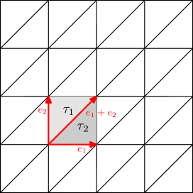
Figure 1. Affine topes for $X=[e_{1},e_{2},e_{1}+e_{2}]$

The choice of the Lebesgue measure $dv$ on $V$ allows us to identify distributions and generalized functions: if $F$ is a generalized function, $Fdv$ is a distribution. If the distribution $Fdv$ is given by ${\langle}Fdv,test{\rangle}=\int_{V}f(v)test(v)dv$, with $f(v)$ locally $L^{1}$, we say that $F$ is locally $L^{1}$, and we use the same notation for $F$ and the locally $L^{1}$ function $f$.

A generalized function $b$ on $V$ will be called piecewise polynomial (relative to $X,\Lambda$) if:

$\bullet$ the function $b$ is locally $L^{1}$,

$\bullet$ on each tope $\tau$, there exists a polynomial function $b(\tau)$ on $V$ such that the restriction of $b$ to $\tau$ coincides with the restriction of the polynomial $b(\tau)$ to $\tau$.

If $F$ is a piecewise polynomial function, we will say that the distribution $Fdv$ is piecewise polynomial.

If $X$ generates $V$, the Box Spline $B(X)$ is a piecewise polynomial (relative to $(X,\Lambda)$) distribution supported on the zonotope $Z(X)$.

Let $f$ be a smooth function on $V$. Then there is two distributions naturally associated to $X,\Lambda,f$:

$\bullet$ the piecewise polynomial distribution $B(X)*_{d}f$:

on a test function $test$,

$${\langle}B(X)*_{d}f,test{\rangle}=\sum_{\lambda\in\Lambda}f(\lambda)\int_{t_{1}=0}^{1}\cdots\int_{t_{N}=0}^{1}test(\lambda+\sum_{i=1}^{N}t_{i}a_{i})dt_{1}\cdots dt_{N}.$$

$\bullet$ the smooth density $B(X)*_{c}f$:

on a test function $test$,

$${\langle}B(X)*_{c}f,test{\rangle}=\int_{V}f(v)\int_{t_{1}=0}^{1}\cdots\int_{t_{N}=0}^{1}test(v+\sum_{i=1}^{N}t_{i}a_{i})dt_{1}\cdots dt_{N}dv.$$

The notations $*_{d}$ and $*_{c}$ means discrete, versus continuous. $B(X)*_{d}f$ is the convolution of $B(X)$ with the discrete measure $\sum_{\lambda}f(\lambda)\delta_{\lambda}$, while $B(X)*_{c}f$ is the usual convolution of $B(X)$ with the smooth density $f(v)dv$. The subscript $*_{c}$ is just for emphasis. The operation $*_{d}$ is denoted $*^{\prime}$ in [5], [6] and is called semi-discrete convolution.

Our aim is to write an explicit formula for the difference $B(X)*_{d}f-B(X)*_{c}f$.

We also associate to $a\in X$ three operators:

$\bullet$ the partial differential operator

$$(\partial_{a}f)(v)=\frac{d}{d\epsilon}f(v+\epsilon a),$$

$\bullet$ the difference operator

$$(\nabla_{a}f)(v)=f(v)-f(v-a),$$

$\bullet$ the integral operator

$$(I_{a}f)(v)=\int_{0}^{1}f(v-ta)dt.$$

The operator $I_{a}$ is the convolution $B([a])*_{c}f$ with the Box Spline associated to the sequence with a single element $a$.

These three operators respects the space of polynomial functions ${\mathbb{C}}[V]$ on $V$. The Taylor series formula implies that, on the space ${\mathbb{C}}[V]$, the operator $I_{a}$ is the invertible operator given by

$$I_{a}=\frac{1-e^{-\partial_{a}}}{\partial_{a}}=\sum_{j=0}^{\infty}(-1)^{j}\frac{1}{(j+1)!}\partial_{a}^{j}.$$

In particular, if $f\in{\mathbb{C}}[V]$ is a polynomial

(2) $$B(X)*_{c}f=\left((\prod_{a\in X}\frac{1-e^{-\partial_{a}}}{\partial_{a}})f\right)dv.$$

If $I,J$ are subsequences of $X$, we define the operators $\partial_{I}=\prod_{a\in I}\partial_{a}$ and $\nabla_{J}=\prod_{b\in J}\nabla_{b}$. They are defined on distributions.

Recall that $\partial_{Y}B(X)=\nabla_{Y}B(X\setminus Y)$, if $Y$ is a subsequence of $X$.

A subsequence $Y$ of $X$ will be called long if the sequence $X\setminus Y$ do not generate the vector space $V$. A long subsequence $Y$, minimal along the long subsequences, is also called a cocircuit: then $Y=X\setminus H$ where $H$ is an admissible hyperplane.

In our formula, when $f$ is a polynomial, $B(X)*_{d}f-B(X)*_{c}f$ is naturally expressed in function of the derivatives $\partial_{Y}f$ with respect to long subsequences $Y$.

2. Piecewise smooth distributions

Our aim is to write an explicit formula for the difference of the two distributions $B(X)*_{d}f$ and $B(X)*_{c}f$. As the first one is a piecewise polynomial distribution, the second a smooth density, we will need to introduce an intermediate space of distributions. We will use ”piecewise smooth distributions”. Let us give a definition.

We continue to assume that $X$ generates $V$.

Definition 2.1.

A generalized function $b$ on $V$ will be called piecewise smooth (relative to $X,\Lambda$) if:

$\bullet$ the generalized function $b$ is locally $L^{1}$,

$\bullet$ on each tope $\tau$, there exists a smooth function $b(\tau)$ on the full space $V$ such that the restriction of $b$ to $\tau$ coincides with the restriction of the smooth function $b(\tau)$ to $\tau$.

In this definition, given a tope $\tau$, the function $b$ restricted to $\tau$ (as well as all its derivatives) extends continuously to the closure of $\tau$. However, these extensions do not always coincide on intersections of the closures of topes.

If $b$ is piecewise smooth, we then say that the distribution $B:=b(v)dv$ (given by integration against the locally $L^{1}$ function $b$) is piecewise smooth.

It is clear that if we multiply a piecewise polynomial distribution $B$ by a smooth function, we obtain a piecewise smooth distribution. Remark that the space of piecewise smooth distributions is stable by the operators $\nabla_{a}$, and by convolution with Box Splines $B(Y)$ ($Y$ any subsequence of $X$). However, it is not stable under operators $\partial_{a}$. For example, $\partial_{X}B(X)=\nabla_{X}B(\emptyset)$ is a linear combination of $\delta$ distributions.

3. Multiple Bernoulli periodic polynomials

Let $U$ be the dual vector space to $V$ and $\Gamma\subset U$ be the dual lattice to $\Lambda$.

If $Y$ is a subsequence of $X$, we define

$$U_{{\mathrm{reg}}}(Y)=\{u\in U\,;{\langle}a,u{\rangle}\neq 0,\;\mbox{for all}\;a\in Y\}$$

and

$$\Gamma_{{\mathrm{reg}}}(Y)=\Gamma\cap U_{{\mathrm{reg}}}(Y).$$

Consider the periodic function on $V$ given by the (oscillatory) sum

(3) $${W}(X)(v)=\sum_{\gamma\in\Gamma_{{\mathrm{reg}}}(X)}\frac{e^{2i\pi{\langle}v,\gamma{\rangle}}}{\prod_{a\in X}2i\pi{\langle}a,\gamma{\rangle}}.$$

This is well defined as a generalized function on $V$. In the sense of generalized functions, we have

(4) $$\partial_{X}W(X)(v)=\sum_{\gamma\in\Gamma_{{\mathrm{reg}}}(X)}e^{2i\pi{\langle}\gamma,v{\rangle}}.$$

We will use this equation to construct “primitives” of parts of the Poisson formula.

We will call the series $W(X)$ a multiple Bernoulli series. Multiple Bernoulli series have been extensively studied by A. Szenes [7]. They are natural generalizations of Bernoulli series: for $\Lambda={\mathbb{Z}}\omega$ and $X_{k}:=[\omega,\omega,\ldots,\omega]$, where $\omega$ is repeated $k$ times with $k>0$, the series

$$W(X_{k})(t\omega)=\sum_{n\neq 0}\frac{e^{2i\pi nt}}{(2i\pi n)^{k}}$$

is equal to $-\frac{1}{k!}B(k,t-[t])$ where $B(k,t)$ denotes the $k^{\text{th}}$ Bernoulli polynomial in variable $t$. In particular, for $k=1$, we have $W(X_{1})(t\omega)=\frac{1}{2}-t+[t]$ (see Figure 2).

Figure 2. Graph of $W(X_{1})(t\omega)=\frac{1}{2}-t+[t]$

We recall the following proposition [7] (see also [2], [1]).

Proposition 3.1.

If $X$ generates $V$, the generalized function $W(X)$ is piecewise polynomial (relative to $(X,\Lambda)$).

Thus we will also call $W(X)$ a multiple periodic Bernoulli polynomial.

The above proposition is proved by reduction to the one variable case. Indeed, the function $\frac{1}{\prod_{a\in X}{\langle}a,z{\rangle}}$ can be decomposed in a sum of functions $\frac{1}{\prod_{i=1}^{n}{\langle}a_{j_{i}},z{\rangle}^{n_{i}}}$ with respect to a basis $a_{j_{i}}$ of $V$ extracted from $X$. This reduces the computation to the one dimensional case. A. Szenes [7] gave an efficient multidimensional explicit residue formula to compute $W(X)$.

Example 3.2.

Let $V={\mathbb{R}}e_{1}\oplus{\mathbb{R}}e_{2}$ with lattice $\Lambda={\mathbb{Z}}e_{1}\oplus{\mathbb{Z}}e_{2}$. Let $X=[e_{1},e_{2},e_{1}+e_{2}]$. We write $v\in V$ as $v=v_{1}e_{1}+v_{2}e_{2}$.

We compute the generalized function

$$\begin{array}[]{ll}W(v_{1},v_{2})&=\displaystyle\sum_{n_{1}\neq 0,n_{2}\neq 0,n_{1}+n_{2}\neq 0}\frac{e^{2i\pi(n_{1}v_{1}+n_{2}v_{2})}}{(2i\pi n_{1})(2i\pi n_{2})(2i\pi(n_{1}+n_{2}))}.\end{array}$$

Then $W$ is a locally $L^{1}$-function on $V$, periodic with respect to ${\mathbb{Z}}e_{1}+{\mathbb{Z}}e_{2}$. To describe it, it is sufficient to write the formulae of $W(v_{1},v_{2})$ for $0<v_{1}<1$ and $0<v_{2}<1$, which we compute (for example using the relation $\frac{1}{n_{1}n_{2}(n_{1}+n_{2})}=\frac{1}{n_{1}(n_{1}+n_{2})^{2}}+\frac{1}{n_{2}(n_{1}+n_{2})^{2}}$) as :

$$W(v_{1},v_{2})=\left\{\begin{array}[]{cl}-\frac{1}{6}(1+v_{1}-2v_{2})(v_{1}-1+v_{2})(2v_{1}-v_{2}),&v_{1}<v_{2}\\ -\frac{1}{6}(v_{1}-2v_{2})(v_{1}-1+v_{2})(2v_{1}-1-v_{2}),&v_{1}>v_{2}.\end{array}\right.$$

Thus we see that $W$ is a piecewise polynomial function.

Remark 3.3.

If $X$ do not generate $V$, $W(X)$ is not locally $L^{1}$: take $X=\emptyset$, then, by Poisson formula, $W(\emptyset)$ is the delta distribution of the lattice $\Lambda$.

Definition 3.4.

A subspace ${\bf{s}}$ of $V$ generated by a subsequence of elements of $X$ is called $X$-admissible. We denote by ${\mathcal{R}}$ the set of $X$-admissible subspaces of $V$. We denote by ${\mathcal{R}}^{\prime}$ the set of proper $X$-admissible subspaces.

The spaces ${\bf{s}}=V$ and ${\bf{s}}=\{0\}$ are among the admissible subspaces of $V$. The set ${\mathcal{R}}^{\prime}$ consists of all admissible subspaces of $V$, except ${\bf{s}}=V$.

Let ${\bf{s}}$ be an admissible subspace of $V$. Let us consider the list $X\setminus{\bf{s}}$, where we have removed from the list $X$ all elements belonging to ${\bf{s}}$. The projection of the list $X\setminus{\bf{s}}$ on $V/{\bf{s}}$ will be denoted by $X/{\bf{s}}$. The image of the lattice $\Lambda$ in $V/{\bf{s}}$ is a lattice in $V/{\bf{s}}$. If $X$ generates $V$, $X/{\bf{s}}$ generates $V/{\bf{s}}$. Using the projection $V\to V/{\bf{s}}$, we identify the piecewise polynomial function $W(X/{\bf{s}})$ on $V/{\bf{s}}$ to a piecewise polynomial function on $V$ constant along the affine spaces $v+{\bf{s}}$.

Define $U_{\rm reg}(X/{\bf{s}})=U_{{\mathrm{reg}}}(X\setminus{\bf{s}})\cap{\bf{s}}^{\perp}$. Thus $\Gamma_{\rm reg}(X/{\bf{s}}):=\Gamma\cap U_{\rm reg}(X/{\bf{s}})$ is the set of elements $\gamma\in\Gamma$ such that:

$${\langle}\gamma,s{\rangle}=0\,\,\,\,{\rm for\,all\,}\,s\in{\bf{s}};\hskip 14.22636pt{\langle}\gamma,a{\rangle}\neq 0\,\,\,{\rm for\,all}\,a\in X\setminus{\bf{s}}.$$

Identifying the dual space to $V/{\bf{s}}$ to the space ${\bf{s}}^{\perp}$, we see that the function $W(X/{\bf{s}})$ is the function on $V$ given by the series (convergent in the sense of generalized functions)

$$W(X/{\bf{s}})(v):=\sum_{\gamma\in\Gamma_{\rm reg}(X/{\bf{s}})}\frac{e^{2i\pi{\langle}v,\gamma{\rangle}}}{\prod_{a\in X\setminus{\bf{s}}}2i\pi{\langle}a,\gamma{\rangle}}.$$

This function is periodic with respect to the lattice $\Lambda$, piecewise polynomial on $V$ (relative to $X$,$\Lambda$) and constant along $v+{\bf{s}}$.

If ${\bf{s}}=V$, the function $W(X/{\bf{s}})$ is identically equal to $1$, while if ${\bf{s}}=\{0\}$, we obtain back our series $W(X)$.

4. A Formula

Let us now state our formula. We assume, as before, that $X$ generates $V$.

For each ${\bf{s}}\in{\mathcal{R}}$, we consider all possible decompositions of the list $X\setminus{\bf{s}}$ in disjoint lists $I\sqcup J$. If $f$ is a smooth function, the function

$$F(v)=W(X/{\bf{s}})(v)(\partial_{I}\nabla_{J}f)(v)$$

is a piecewise smooth function on $V$. If $Y$ is a subsequence of $X$, the convolution $B(Y)*Fdv$ is well defined and the result is a piecewise smooth distribution on $V$ that we denote by $B(Y)*_{c}(W(X/{\bf{s}})\partial_{I}\nabla_{J}f).$

Theorem 4.1.

Let $f$ be a smooth function on $V$. We have

$$B(X)*_{d}f-B(X)*_{c}f=\sum_{{\bf{s}}\in\mathcal{R}^{\prime}}\sum_{I\subset X\setminus{\bf{s}}}(-1)^{|I|}B((X\cap{\bf{s}})\sqcup I)*_{c}(W(X/{\bf{s}})\partial_{I}\nabla_{J}f).$$

In this formula $J$ is the complement of the sequence $I$ in $X\setminus{\bf{s}}$.

This equality holds in the space of piecewise (relative to $(X,\Lambda)$) smooth distributions on $V$, relative to $(X,\Lambda)$.

Remark 4.2.

If $f$ is a polynomial, the term $B(X)*_{c}f$ is a polynomial density and all terms of the difference formula are locally polynomial distributions on $V$.

Before proceeding, let us comment on the proof. As in [3] (see also [5]), we use the Poisson formula to compute $B(X)*_{d}f$. Then we group the terms in the dual lattice $\Gamma$ in strata according to the hyperplane arrangement $\cup_{a\in X}\{a=0\}$. We then use the Bernoulli series as primitives of the corresponding sums. This way, we introduce the needed derivatives of the function $f$.

Proof.

Let ${\mathcal{R}}$ be the set of admissible subspaces of $V$. We have the disjoint decomposition:

(5) $$U=\bigsqcup_{{\bf{s}}\in\mathcal{R}}U_{{\mathrm{reg}}}(X/{\bf{s}}).$$

Let $test$ be a test function on $V$. We compute

$$S:=\int_{V}(B(X)*_{d}f)(v)test(v)=\sum_{\lambda\in\Lambda}f(\lambda)\int_{V}B(X)(v)test(\lambda+v).$$

We apply Poisson formula to the compactly supported smooth function

$$q(w)=f(w)\int_{V}B(X)(v)test(w+v)$$

as our sum $S$ is equal to $\sum_{\lambda\in\Lambda}q(\lambda).$ We obtain

$$S=\sum_{\gamma\in\Gamma}\int_{V}e^{2i\pi{\langle}w,\gamma{\rangle}}q(w)dw.$$

The lattice $\Gamma$ is a disjoint union of the sets $\Gamma_{{\mathrm{reg}}}(X/{\bf{s}})=\Gamma\cap U_{{\mathrm{reg}}}(X/{\bf{s}})$ associated to the admissible subspaces ${\bf{s}}$. Remark that the set associated to ${\bf{s}}=V$ is $\{\gamma=0\}$. The term in $S$ corresponding to $\gamma=0$ is $\int_{V}q(w)dw$, that is ${\langle}B(X)*_{c}f,test{\rangle}$.

As in the generalized function sense

$$\sum_{\gamma\in\Gamma_{{\mathrm{reg}}}(X/{\bf{s}})}e^{2i\pi{\langle}w,\gamma{\rangle}}=\partial_{X\setminus{\bf{s}}}W(X/{\bf{s}})(w),$$

we obtain

$$S=\sum_{{\bf{s}}\in\mathcal{R}}\int_{V}W(X/{\bf{s}})(w)(-1)^{|X\setminus{\bf{s}}|}\partial_{X\setminus{\bf{s}}}q(w)dw.$$

The function $q(w)$ is product of the two smooth functions $f(w)$ and $\int_{V}B(X)(v)test(w+v).$ By Leibniz rule,

$$S:=\sum_{{\bf{s}}}(-1)^{|X\setminus{\bf{s}}|}\sum_{I\sqcup J=X\setminus{\bf{s}}}\int_{V}\int_{V}W(X/{\bf{s}})(w)\partial_{I}f(w)B(X)(v)\partial_{J}test(w+v)dw.$$

We first integrate in $v$ and use the equation satisfied by the Box Spline

$${\langle}B(X),\partial_{b}h{\rangle}=-{\langle}B(X\setminus\{b\}),\nabla_{-b}h{\rangle}.$$

Thus we obtain

$$S=\sum_{{\bf{s}}}\sum_{I\sqcup J=X\setminus{\bf{s}}}(-1)^{|I|}\int_{V}\int_{V}W(X/{\bf{s}})(w)\partial_{I}f(w)B(X\setminus J)(v)(\nabla_{-J}test)(w+v)dw.$$

Let us integrate in $w$. We use the invariance of the integral by $\nabla_{b}$ : $\int_{V}(\nabla_{b}f_{1})(w)f_{2}(w)dw=\int_{V}f_{1}(w)(\nabla_{-b}f_{2})(w)dw.$ As $b\in J$ is in $\Lambda$, and $W(X/{\bf{s}})(w)$ is periodic,

$$S=\sum_{{\bf{s}}\in\mathcal{R}}\sum_{I\sqcup J=X\setminus{\bf{s}}}(-1)^{|I|}\int_{V}\int_{V}B(X\setminus J)(v)W(X/{\bf{s}})(w)\nabla_{J}\partial_{I}f(w)test(w+v)dw.$$

Writing $\mathcal{R}=\{V\}\sqcup\mathcal{R}^{\prime}$, we obtain the formula of the theorem.

∎

On the space of polynomials, one has

$$\nabla_{J}\partial_{I}f=(\prod_{b\in J}\frac{1-e^{-\partial_{b}}}{\partial_{b}})\partial_{X\setminus{\bf{s}}}f$$

if $I\sqcup J=X\setminus{\bf{s}}$.

Recall that the space $D(X)$ of Dahmen-Micchelli polynomials is the space of polynomials on $V$ such that $\partial_{Y}f=0$ for all long subsequences $Y$. In particular, if ${\bf{s}}$ is a proper subspace, the sequence $X\setminus{\bf{s}}$ is a long subsequence. So if $I,J$ are such that $I\sqcup J=X\setminus{\bf{s}}$ and $f\in D(X)$, then $\nabla_{J}\partial_{I}f=0$.

As a corollary of our formula, if $p\in D(X)$, we see that $B(X)*_{d}p=B(X)*_{c}p$. Let us state more precisely this result of Dahmen-Micchelli [4] (see also [6], chapter 16).

Corollary 4.3.

If $p\in D(X)$, then

$$P(v):=B(X)*_{d}p=\sum_{\lambda}p(\lambda)B(X)(v-\lambda)$$

is a polynomial function on $V$, equal to $(\prod_{a\in X}\frac{1-e^{-\partial_{a}}}{\partial_{a}})p=B(X)*_{c}p.$

In this formula, we have identified $B(X)$, $B(X)*_{d}p$, and $B(X)*_{c}p$ to piecewise polynomial functions.

5. Vertices of the arrangement and semi-discrete convolutions.

We now give a twisted version of Theorem 4.1, where we twist $f$ by an exponential function $e^{2i\pi{\langle}G,v{\rangle}}$.

The set of characters on $\Lambda$ is the torus $T:=U/\Gamma$. If $g\in T$, we denote by $g^{\lambda}$ the corresponding character on $\Lambda$. More precisely if $g$ has representative $G\in U$, then by definition $g^{\lambda}=e^{2i\pi{\langle}G,\lambda{\rangle}}$. Define

$$X(g):=\{a\in X;g^{a}=1\}.$$

If $g\in T=U/\Gamma$ has representative $G\in U$, we denote by $g+\Gamma$ the set $G+\Gamma$.

For $a\in X$, introduce the operator

$$(\nabla(a,g)f)(v)=f(v)-g^{-a}f(v-a).$$

If $Y$ is a subsequence of $X$, define

$$\nabla_{Y}^{g}=\prod_{a\in Y}\nabla(a,g).$$

We introduce a subset $\mathcal{R}(g)$ of admissible subspaces, depending on $g$.

Definition 5.1.

The admissible space ${\bf{s}}$ is in $\mathcal{R}(g)$ if the space $(g+\Gamma)\cap{\bf{s}}^{\perp}$ is non empty

Remark that if $G$ is not in $\Gamma$, then $V$ is not in the set ${\mathcal{R}}(g)$.

Remark 5.2.

If ${\bf{s}}\in\mathcal{R}(g)$, then all elements of $X\cap{\bf{s}}$ are in $X(g)$. Thus $\mathcal{R}(g)$ is contained in the set of admissible spaces for $X(g)$. However the converse does not hold: take $V={\mathbb{R}}\omega$ $X=[2\omega]$, $\Lambda={\mathbb{Z}}\omega$, and $G=\frac{1}{2}\omega^{*}$. Then $X(g)=X$, so that $V$ is an admissible subspace for $X(g)$. However, $V$ is not in ${\mathcal{R}}(g)$.

If ${\bf{s}}\in\mathcal{R}(g)$, take $g_{\bf{s}}\in(g+\Gamma)\cap{\bf{s}}^{\perp}$. Then $(g+\Gamma)\cap{\bf{s}}^{\perp}$ is the translate by $g_{\bf{s}}$ of the lattice $\Gamma\cap{\bf{s}}^{\perp}$.

Define

$$\Gamma_{{\mathrm{reg}}}(X/{\bf{s}},g)=(g+\Gamma)\cap U_{{\mathrm{reg}}}(X/{\bf{s}})^{\perp}.$$

Thus $\Gamma_{{\mathrm{reg}}}(X/{\bf{s}},g)$ consists of elements $\xi\in g+\Gamma$ such that

$${\langle}\xi,s{\rangle}=0\,\,\,\,{\rm for\,all\,}\,s\in{\bf{s}};\hskip 14.22636pt{\langle}\xi,a{\rangle}\neq 0\,\,\,{\rm for\,all}\,a\in X\setminus{\bf{s}}.$$

The following series

(6) $${W}(X/{\bf{s}},g)(v)=\sum_{\xi\in\Gamma_{{\mathrm{reg}}}(X/{\bf{s}},g)}\frac{e^{2i\pi{\langle}v,\xi{\rangle}}}{\prod_{a\in X}2i\pi{\langle}a,\xi{\rangle}}$$

is well defined as a generalized function on $V$.

The function ${W}(X/{\bf{s}},g)(v)$ is not periodic with respect to $\Lambda$. We have instead the covariance formula

(7) $$W(X/{\bf{s}},g)(v-\lambda)=g^{-\lambda}W(X/{\bf{s}},g)(v).$$

In the sense of generalized functions, we have

(8) $$\partial_{X\setminus{\bf{s}}}W(X/{\bf{s}},g)(v)=\sum_{\xi\in\Gamma_{{\mathrm{reg}}}(X/{\bf{s}},g)}e^{2i\pi{\langle}\xi,v{\rangle}}.$$

We recall the following proposition [7] (see also [2],[1]).

Proposition 5.3.

The generalized function $W(X/{\bf{s}},g)$ is a piecewise polynomial (relative to $(X,\Lambda)$) function on $V$.

It is proven similarly by reduction to one variable.

Example 5.4.

Let $V={\mathbb{R}}\omega$, $\Lambda={\mathbb{Z}}\omega$ and $X_{k}:=[\omega,\omega,\ldots,\omega]$, where $\omega$ is repeated $k$ times with $k>0$. Then $\Gamma={\mathbb{Z}}\omega^{*}$. Then if $z$ is not an integer

$$W(X_{k},z\omega^{*})(t\omega)=\sum_{n\in{\mathbb{Z}}}\frac{e^{2i\pi(n+z)t}}{(2i\pi(n+z))^{k}}.$$

We have, for example, (see [2])

$$W(X_{1},z\omega^{*})(t\omega)=\frac{e^{2i\pi[t]z}}{1-e^{-2i\pi z}}.$$

$$W(X_{2},z\omega^{*})(t\omega)=e^{2i\pi[t]z}(\frac{t-[t]}{1-e^{-2i\pi z}}+\frac{1}{(1-e^{-2i\pi z})(1-e^{2i\pi z})}).$$

Here $[t]$ is the integral part of $t$. This function $[t]$ is a constant on each interval $]\ell,\ell+1[$, and $W(X_{k},z\omega^{*})$ is a locally polynomial function of $t$.

Theorem 5.5.

Let $G\in U$, and $g$ its image in $U/\Gamma.$ Let $f(v)=e^{2i\pi{\langle}v,G{\rangle}}h(v)$, where $h$ is a smooth function. Then

$$B(X)*_{d}f=\sum_{{\bf{s}}\in\mathcal{R}(g)}\sum_{I\subset X\setminus{\bf{s}}}(-1)^{|I|}B((X\cap{\bf{s}})\sqcup I)*_{c}(W(X/{\bf{s}},g)\partial_{I}\nabla_{J}^{g}h).$$

In this formula, $J$ is the complement of $I$ in $X\setminus{\bf{s}}$.

Remark 5.6.

If $G\in\Gamma$, then $B(X)*_{d}f=B(X)*_{d}h$, and the formula of the theorem above coincide with the formula of Theorem 4.1 for $h$: the set $\mathcal{R}(g)$ coincide with the set $\mathcal{R}$, and the term corresponding to $V$ in the formula of Theorem 5.5 is $B(X)*_{c}h$.

Proof.

We proceed in the same way than the proof of Theorem 4.1. Let $test$ be a test function on $V$. We compute $S:=\int_{V}(B(X)*_{d}f)(v)test(v)$ by Poisson formula. If

$$q(w)=h(w)\int_{V}B(X)(v)test(w+v),$$

we obtain

$$S=\sum_{\gamma\in\Gamma}\int_{V}e^{2i\pi{\langle}w,\gamma{\rangle}}e^{2i\pi{\langle}w,G{\rangle}}q(w)dw.$$

Thus

$$S=\sum_{\xi\in(g+\Gamma)}\int_{V}e^{2i\pi{\langle}w,\xi{\rangle}}q(w)dw.$$

The set $g+\Gamma$ is a disjoint union over ${\bf{s}}\in\mathcal{R}(g)$ of the sets $\Gamma_{{\mathrm{reg}}}(X/{\bf{s}},g)=(g+\Gamma)\cap U_{{\mathrm{reg}}}(X/{\bf{s}})$, so

$$S=\sum_{{\bf{s}}\in\mathcal{R}(g)}\int_{V}W(X/{\bf{s}},g)(w)(-1)^{|X\setminus{\bf{s}}|}\partial_{X\setminus{\bf{s}}}q(w)dw.$$

Then, using Leibniz rule for $\partial_{a}$ , and equation for the Box Spline, we obtain that $S$ is equal to

$$\sum_{{\bf{s}}\in\mathcal{R}(g)}\sum_{I\sqcup J=X\setminus{\bf{s}}}(-1)^{|I|}\int_{V}\int_{V}W(X\setminus{\bf{s}},g)(w)\partial_{I}f(w)B(X\setminus J)(v)(\nabla_{-J}test)(w+v)dw.$$

Using the covariance formula (7) for $W(X\setminus{\bf{s}},g)$, we see that

$$\int_{V}W(X\setminus{\bf{s}},g)(w)f_{1}(w)(\nabla_{-b}f_{2})(w)dw=\int_{V}W(X\setminus{\bf{s}},g)(w)(\nabla(b,g)f_{1})(w)f_{2}(w)dw$$

and we obtain the formula of the theorem. ∎

Let us point out a corollary of this formula.

Definition 5.7.

We say that a point $g\in U/\Gamma$ is a toric vertex of the arrangement $X$, if $X(g)$ generates $V$. We denote by $\mathcal{V}(X)$ the set of toric vertices of the arrangement $X$.

If $g$ is a vertex, there is a basis $\sigma$ of $V$ extracted from $X$ such that $g^{a}=1$, for all $a\in\sigma$. We thus see that the set $\mathcal{V}(X)$ is finite.

If $X$ is unimodular, then $\mathcal{V}(X)$ is reduced to $g=0$.

Corollary 5.8.

(Dahmen-Micchelli)

Let $g\in\mathcal{V}(X)$ be a toric vertex of the arrangement $X$ and let $p\in D(X(g))$ be a polynomial in the Dahmen-Micchelli space for $X(g)$. Assume that $g\neq 0$. Let $f(\lambda)=g^{\lambda}p(\lambda)$. Then $B(X)*_{d}f=0$

Proof.

We apply the formula of Theorem 5.5 with $h=p$. As $g\neq 0$, all terms ${\bf{s}}\in\mathcal{R}(g)$ are proper subspaces of $V$. Let us show that all the terms in our formula are $0$. Indeed let $I\sqcup J=X\setminus{\bf{s}}$. Let $I^{\prime}=I\cap X(g)$ and $J^{\prime}=J\cap X(g)$. Then $I^{\prime}\sqcup J^{\prime}=X(g)\setminus{\bf{s}}$ is a long subset of $X(g)$. As $\nabla_{I^{\prime}}^{g}=\nabla_{I^{\prime}}$, we see that $\partial_{I^{\prime}}\nabla_{J^{\prime}}^{p}$ is already equal to $0$.

∎

I wish to thank Michel Duflo for comments on this text.

Michèle Vergne, Institut de Mathématiques de Jussieu, Théorie des Groupes, Case 7012, 2 Place Jussieu, 75251 Paris Cedex 05, France;

email: vergne@math.jussieu.fr

References

[1] Boysal A., Vergne M.,
Wall crossing formula for Multiple Bernoulli series. to appear
[2] Brion M. and Vergne M., Arrangement of hyperplanes II: The Szenes formula and Eisenstein series.
Duke Math. J. 103 (2000), no. 2, 279–302.
[3]Dahmen W., Micchelli C., Translates of multivariate splines, Linear Algebra Appl.52 (1983), no. 2, 217–234.
[4]
Dahmen W., Micchelli C.,
On the solution of certain systems of partial difference
equations and linear dependence of translates of box splines,
Trans. Amer. Math. Soc., 292,
1985,
1, 305–320.