Macroscopic Interferences of Neutrino Waves

Abstract

Interference phenomena of neutrinos are studied. High energy neutrino in T2K near detector and low energy neutrino in KamLAND are possible experiments that could show macroscopic interferences of neutrino waves. In both experiments interference patterns may give new insights on the absolute value of the neutrino mass.

1 Interference of neutrino waves

If a wave function $\psi_{\nu}(t,{\vec{x}})$ is a sum of two different wave functions, the probability of observing this particle that is proportional to $|\psi(t,{\vec{x}})|^{2}$ has an interference term. Interference phenomena of the light, electron, and neutron have been studied well and are used for many purposes in wide area. The neutrino is a wave and interacts with matters so weakly that it is extremely difficult to control the neutrino. It is a challenging task to prepare a detection method for the neutrino interference.

In this article, we show that diffraction-like experiments of neutrinos are possible despite its extreme weakness of interactions with matters [1][2] and that they give new insights on neutrinos. Due to the weakness of the interactions it is necessary to analyze whole processes from its production to detection [3]. Neutrino becomes a wave packet of a finite coherence length and behaves as a wave and particle simultaneously. Its coherence properties are important for the observability of the interferences. Neutrino is produced in the scattering or decay of a particle by the weak interaction and is in the intermediate state between the production and detection processes[4] as is shown in Fig. 1,

$$particle+target\rightarrow neutrino\rightarrow neutrino+target\rightarrow particles.$$ (1)

For the interference pattern of the neutrino to become observable, a wave at the detector should be a superposition of multiple waves of different phases.

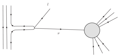
Fig. 1: The whole processes of the neutrino reaction is shown. The neutrino is produced as a decay product of the pion or nucleon and propagates for macroscopic distance. The neutrino is detected finally.

Distance, $L$, and energy, $E_{\nu}$, of the neutrino propagations of T2K [5] near detector and KamLAND [6], which we focus in the present work are

$$\text{T2K}\,:\,L=few\times 100\,[\text{m}].;~{}E_{\nu}=few\times[\text{GeV}/c],$$ (2)

$$\text{KamLAND}\,:\,L=200[\text{km}].;~{}E_{\nu}=few\times[\text{MeV}/c].$$ (3)

$L$ is the distance between the reactor and detector in KamLAND, and is shorter than the distance between pion source and detector in T2K, since pions decay in large decay area. These parameters are different each others but two experiments show similar phenomena of interferences.

2 Neutrino production and detection :wave packet scattering

The amplitude of the neutrino reactions from its production to detection is written as

$$\langle l,\alpha_{out},\beta_{out}|\int dx_{1}dx_{2}T(H_{i}(x_{1})H_{i}(x_{2}))|\alpha_{in},\beta_{in}\rangle,$$ (4)

with a weak interaction Hamiltonian $H_{i}(x)$ and the in-states $\alpha_{in},\beta_{in}$ and out-states $\alpha_{out},\beta_{out}$ and a lepton $l$. In the standard S-matrix, the in-states and out-states are plane waves defined at $t=-\infty$ and at $t=\infty$. Hence this amplitude is invariant under the translation of the space and time and is useless for the space-time dependent informations in scatterings such as probability at a finite time interval or finite distance. These translational non-invariant quantities are calculated if the states $\alpha,\beta$ are defined using wave packets [3]. The wave packet is defined around a certain time and position and has the energy and momentum of finite uncertainties and is useful for studying the space time dependent informations. We study the amplitudes of the wave packets and find the finite time or length dependences of the amplitudes.

First the coherence lengths in which the waves keep coherences are evaluated from the production and detection processes. Neutrinos are produced by a decay of particles which have certain coherence lengths. As was analyzed in Ref.[1], the coherence lengths are the sizes of waves that maintain coherence. The mean free path, on the other hand, is calculated from the transition probability and the density of scatterers as the average distance that a particular wave propagates freely. Hence the coherence lengths are determined by mean free paths.

(1-1)Decay of pion in fright.

Pion is produced in matter, in metal for instance, and the mean free path was calculated [1] as

$$\sigma_{pion}=10^{-1}[\text{m}].$$ (5)

When these pions are emitted from metal into the vacuum, these waves maintain coherence within this size. So the length in which particles maintain coherence is determined by the mean free path. These particles are described by the wave packets of the finite coherence length in the vacuum.

(1-2)Decay of Nucleus in solid.

The other sources of neutrino are unstable nucleus. In reactor, these unstable nucleus are bound in atoms, and they are described by wave functions of finite sizes. The sizes of nucleus wave functions are estimated from the center of mass gravity effect between the nucleus and electrons in the atom [1] as,

$$\sigma_{Nucleus}=r\times R_{atom}={1\over 2000}\times 10^{-10}\approx 10^{-13}[\text{m}],$$ (6)

where $r$ is the ratio between the mass of nucleus and electrons and $R_{atom}$ is the size of atom. The size of nucleus wave packet is in the range between the nucleus size and atom size. So, the size of pion wave packet in fright is large but the size of nucleus wave packet is small.

Neutrinos interact with particles in the target such as electrons or nucleus which have finite coherence lengths. The electron has a large size but the nucleus has a small size, and they are defined by wave packets.

(2-1)Electron wave function in matter.

Bound electrons in atom are described by atomic wave functions. The wave packet of the electron has a size of the electron wave function

$$\sigma_{electron}=10^{-10}[\text{m}].$$ (7)

(2-2) Nuclear wave function in solid

Nucleus is extremely small and is described by a nucleus wave function. From the size of nucleus wave function Eq.$(\ref{nucleus-size})$, the wave packet of nucleus has a size

$$\sigma_{Nucleus}=10^{-13}[\text{m}],$$ (8)

which is the same as Eq. (6). Thus the nucleus has a small size.

Wave packet is a superposition of plane waves with a momentum dependent weight. Gaussian and Lorentzian wave packets are studied often. They become maxima around the central region and decrease uniformly at large momentum region. The former decreases rapidly but the latter decreases slowly. In the central region , Gaussian wave packet is most convenient for practical calculations and is applied here also. In the tail region, where the momentum becomes large, the particle correlations are determined here from their production processes.

The tail of the wave packet of pion that is produced in hadron collisions depends on the production processes. They are described by pion correlation functions

$$\Delta_{p}(x_{1}-x_{2})=\langle\alpha|\varphi(x_{1})|\beta\rangle\langle\beta|\varphi(x_{2})|\alpha\rangle,$$ (9)

for the initial and final state $|\alpha\rangle,|\beta\rangle$ and is transformed as

$$\Delta_{p}(x_{1}-x_{2})=\int d^{4}qe^{ip(x_{1}-x_{2})}\Delta_{p}(q).$$ (10)

The $\Delta(q)$ of a free relativistic particle, $\Delta_{p}^{(free)}(q)$, and of an interacting particle with $\varphi^{4}(x)$ interaction, $\Delta_{p}^{(int)}(q)$, are

$$\Delta^{(free)}(q)={1\over(2\pi)^{4}}{1\over q^{2}-m^{2}-i\epsilon},$$ (11)

$$\Delta^{(int)}(q)={1\over(2\pi)^{4}}{1\over q^{2}-m^{2}-i\epsilon}{1\over q^{2}-m^{2}+i\epsilon}\delta((q+q_{\delta})^{2}-m^{2}).$$ (12)

From these correlation functions, $\Delta_{p}^{(free)}(x)$ and $\Delta_{p}^{(int)}(x)$ are calculated in Euclidean metric in the limit $\lambda=\sqrt{x^{2}}\rightarrow 0$ as

$$\Delta_{p}^{(free)}(x)={1\over 4\pi}\delta(\lambda)+less~{}singular~{}term,$$ (13)

$$\Delta_{p}^{(int)}(x)={1\over 64\pi^{2}}+O(\lambda),~{}:~{}q_{\delta}\rightarrow 0.$$ (14)

3 Wave packet evolution

A wave packet is a superposition of the momentum states and has a finite spatial width [7][8][9][10]. Although a neutrino wave packet is an intermediate state in our formalism, it is instructive and useful to analyze the wave packet and its evolution in time here. The wave packet behaves like a particle and has the center position of momentum, space, and time. Although it behaves like a particle, it also behaves like a wave and has a characteristic phase. So the wave packet is not the same as an ordinary particle.

Wave packet of the central values of the position, ${\vec{X}}_{0}$, the momentum, ${\vec{P}}_{0}$, and the time, ${\vec{T}}_{0}$ is decomposed as

$$\langle t,{\vec{x}}|{\vec{P}}_{0},{\vec{X}}_{0},T_{0}\rangle=\int d{\vec{p}}\langle{\vec{x}}|{\vec{p}}\rangle\langle t,{\vec{p}}|{\vec{P}}_{0},{\vec{X}}_{0},T_{0}\rangle$$ (15)

$$=N_{3}\left({\sigma\over 2\pi}\right)^{\frac{3}{2}}\int d{\vec{p}}e^{-iE({\vec{p}})(t-T_{0})+i{\vec{p}}\cdot({\vec{x}}-{\vec{X}}_{0})-{\sigma\over 2}({\vec{p}}-{\vec{P}}_{0})^{2}},$$

where $\sigma$ is the size of wave packet. The wave packet maintains its shape and size during small $t-T_{0}$ period, and it has a translational motion.

$$\langle t,{\vec{x}}|{\vec{P}}_{0},{\vec{X}}_{0},T_{0}\rangle=N_{3}e^{-{1\over 2\sigma}({\vec{x}}-{\vec{X}}_{0}-{\vec{v}}_{0}(t-T_{0}))^{2}}e^{-i\phi},$$ (16)

$$\phi=E({\vec{P}}_{0})(t-T_{0})-{\vec{P}}_{0}\cdot({\vec{x}}-{\vec{X}}_{0}),~{}{\vec{v}}_{0}={p_{i}\over E({\vec{p}})}.$$ (17)

The wave is extended around the center ${\vec{x}}(t)={\vec{X}}_{0}+{\vec{v}}_{0}(t-T_{0})$, and is classified by the phase $\phi$. The phase at the center is given by

$${\phi=E({\vec{P}}_{0})(t-T_{0})-{\vec{P}}_{0}\cdot({\vec{x}}-{\vec{X}}_{0})=\left(E-{p^{2}\over E}\right)(t-T_{0})={m^{2}\over E}(t-T_{0})}.$$ (18)

This phase is proportional to the mass squared and inversely proportional to the energy. Hence its magnitude becomes extremely small. At large $t-T_{0}$, the stationary momentum that satisfies

$${\partial\over\partial p_{i}}\left({-iE({\vec{p}})(t-T_{0})+i{\vec{p}}\cdot({\vec{x}}-{\vec{X}}_{0})-{\sigma\over 2}({\vec{p}}-{\vec{P}}_{0})^{2}}\right)=0.$$ (19)

gives a dominant contribution to the above momentum integral. The momentum which satisfies this equation is determined by the time and space coordinates,

$${\vec{P}}_{X}={\vec{P}^{(0)}}_{X}+O\left({1\over t-T_{0}}\right),$$ (20)

$${\vec{P}^{(0)}}_{X}=m{1\over\sqrt{(t-T_{0})^{2}-({\vec{x}}-{\vec{X}}_{0})^{2}}}({\vec{x}}-{\vec{X}}_{0})$$ (21)

and the wave function is described as

$$\langle t,{\vec{x}}|{\vec{P}}_{0},{\vec{X}}_{0},T_{0}\rangle$$ (22)

$$=N_{3}e^{-iE({\vec{p}})(t-T_{0})+i{\vec{p}}\cdot({\vec{x}}-{\vec{X}}_{0})}\left({1\over 2i{\gamma_{L}\over\sigma}+1}\right)^{\frac{1}{2}}\left({1\over 2i{\gamma_{T}\over\sigma}+1}\right)e^{-{1\over 2}\sigma({{\vec{P}^{(0)}}_{X}}-{{\vec{P}}_{0}})^{2}},$$ (23)

This wave has the same phase

$$\phi={m^{2}\over E}(t-T_{0})$$ (24)

as before and the magnitude varies with time. The magnitude decreases and the wave expands with time in space. The expansion parameters in the longitudinal direction, $\gamma_{L}$, and in the transverse direction, $\gamma_{T}$ are

$$\gamma_{L}={1\over 2}{m^{2}|t-T_{0}|\over E^{3}({\vec{P}}_{X})},~{}\gamma_{T}={1\over 2}{|t-T_{|}\over E({\vec{P}}_{X})}.$$ (25)

The longitudinal expansion is proportional to the mass squared and vanishes in the massless case. The transverse expansion is independent from the mass and is determined by the initial size of the wave packet.

4 Probability at finite time interval

Probability at finite time interval :T2K near detector

The transition amplitude of the neutrino reaction which includes the production and detection processes are studied by wave packets [11]. The neutrino is treated as a wave in the intermediate states and its size is determined by the particle and wave properties in the initial and final states.

The amplitude $T$ for a T2K neutrino reaction that includes the production and propagation processes where the neutrino is in the outgoing state is given as

$$T = igm_{\mu}N^{\prime}\int dtd{\vec{x}}d{\vec{p}}_{\nu}\langle\beta_{f}|\varphi(x)|\alpha_{i}\rangle\left(\frac{m_{\nu}}{E(\vec{p}_{\nu})}\right)^{\frac{1}{2}}$$

$$\times e^{i\left(E(\vec{p}_{\mu})t-{\vec{p}}_{\mu}\cdot{\vec{x}}\right)}\bar{u}({\vec{p}}_{\mu})\gamma_{5}\nu({\vec{p}}_{\nu})e^{i\left(E({\vec{p}}_{\nu})(t-T_{\nu})-{\vec{p}}_{\nu}\cdot({\vec{x}}-{\vec{X}}_{\nu})\right)-{\sigma_{\nu}\over 2}({\vec{p}}_{\nu}-{\vec{k}}_{\nu})^{2}},$$

$$N^{\prime} = \frac{N_{\nu}}{(2\pi)^{\frac{3}{2}}}\left(\frac{m_{\mu}}{E(\vec{p}_{\mu})}\right)^{\frac{1}{2}},$$

$$\langle\beta_{f}|\varphi(x)|\alpha_{i}\rangle = \left(\frac{4\pi}{\sigma_{\pi}}\right)^{\frac{3}{4}}e^{-i\left(E({\vec{p}}_{pion})(t-T_{\pi})-{\vec{p}}_{pion}\cdot({\vec{x}}-{\vec{X}}_{\pi})\right)}$$ (27)

$$\times e^{-{1\over 2\sigma_{\pi}}\left({\vec{x}}-{\vec{X}_{\pi}}-{\vec{v}}_{\pi}(t-T_{\pi})\right)^{2}}T_{\beta^{\prime}_{f},\alpha_{i}}.$$

In the above equation, $|\alpha_{i}\rangle$ is the initial state and $|\beta_{f}\rangle$ is the final state. $\varphi(x)$ is the pion field and $(t,{\vec{x}})$ is the space time coordinates where the weak interaction takes place. The pion is expressed by the wave packet of the size $\sigma_{\pi}$ and is produced at the space time coordinate ${(T_{\pi},{\vec{X}}_{\pi})}$. The neutrino is detected with the wave packet of the size $\sigma_{\nu}$ and is detected at $(T_{\nu},{\vec{X}}_{\nu})$.

After the tedious calculations, we have integrated probability of observing neutrino at a finite time T as,

$$\int d{\vec{p}}_{\text{muon}}d{\vec{x}}_{neutrino}d{\vec{p}}_{pion}\sum_{s_{1},s_{2}}|T|^{2}$$ (28)

$$=N\int_{0}^{\text{T}}dt_{1}dt_{2}{e^{i{m_{\nu}^{2}\over E_{\nu}}(t_{1}-t_{2})}\over(t_{1}-t_{2})}\left(1+f_{\text{normal}}e^{i\omega_{\pi}(t_{1}-t_{2})}\right)$$

$$=\frac{\tilde{N}_{\text{prob}}}{E_{\nu}}~{}\left[F_{\text{universal}}(0)\times g(\text{T},\omega_{\nu})+f_{\text{normal}}\times g(\text{T},\omega_{\pi}+\omega_{\nu})\right],$$

$$\tilde{N}_{\text{prob}} = (2\sqrt{2}\pi)^{3}\sigma_{\nu}f_{\mu},~{}f_{\mu}=g^{2}m_{\mu}^{2}(m_{\pi}^{2}-m_{\mu}^{2}),$$

$$g(\text{T},\omega) = \text{T}\int^{\text{T}}_{0}dX\frac{\sin\left(\omega X\right)}{X}+\frac{1}{\omega}\left\{\cos(\omega\text{T})-1\right\},$$ (29)

$$\omega_{\nu} = \frac{m_{\nu}^{2}}{E_{\nu}},~{}\omega_{\pi}=\frac{m_{\pi}^{2}}{E_{\pi}},~{}L=c\text{T},$$

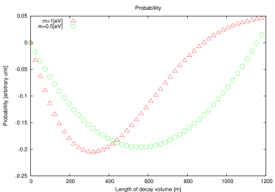
Fig. 2: The length dependence of the oscillating part in the 1 [GeV] neutrino detection probability of the mass $1\,[\text{eV}/c^{2}]$ and $0.5\,[\text{eV}/c^{2}]$ is shown.

where the coefficients $F_{\text{universal}}$ is determined from the large momentum contribution at the tail of the wave packet Eqs.$(\ref{interactig-correlation})$ and $f_{\text{normal}}$ is determined from the states at the central region of the wave packet. The probability at a finite time T has a T-linear term and an oscillating term.

The oscillating term for the mass $1\,[\text{eV}/c^{2}]$ and $0.5\,[\text{eV}/c^{2}]$ is given in Fig. (2). The probability becomes minimum at around $300\,[\text{m}]$ for $1\,[\text{eV}/c^{2}]$ and at around $600\,[\text{m}]$ for $0.5\,[\text{eV}/c^{2}]$ and is expected to be observable.

KamLAND neutrino:flavour oscillation

The neutrino production and detection processes are the second order weak process at the coordinate $x_{1}^{\mu}$ and the detection of the coordinate $x_{2}^{\mu}$. The particle states $\alpha_{i}$ and $\beta_{i}$ in the initial state are defined by the wave packets and integration on the variables, ${\vec{x}}_{1}$ and $x_{2}^{\mu}$ are made easily. The amplitude for KamLAND neutrino becomes, then,

$$T = iN^{\prime}\int dx_{1}^{0}T_{1}\bar{u}({\vec{p}}_{l_{i}})(1-\gamma_{5})\gamma^{\mu_{1}}\int d{\vec{p}}_{\nu}{\gamma p+m_{\nu}\over 2E({\vec{p}}_{\nu})}e^{-ip_{\nu}(X_{1}-X_{2})}$$

$$\times e^{-\sigma_{f}^{p}({\vec{p}}-{\vec{P}_{f}})^{2}}e^{i({p^{0}}-{P_{\alpha}^{0}})x_{1}^{0}}e^{-\sigma_{f}^{0}({p^{0}}-{P_{\beta}^{0}})^{2}}\Gamma u({\vec{p}}_{l_{f}})\tilde{T}_{2},$$

where $X_{1}^{\mu}$ and $X_{2}^{\mu}$ are the space and time coordinates of the particles at production and detection and $T_{1}$ and $T_{2}$ are the amplitudes where the neutrino is produced or detected. The integrand is an exponential function of those that have real parts and imaginary parts and the integral is obtained either around the minimum of the real part, Gaussian point, ${\vec{k}}_{\nu}$, or the minimum of the imaginary part, stationary phase point. The wave packet sizes $\sigma_{f}^{p}$ and $\sigma_{f}^{0}$ are defined from the wave packet sizes of particles. The Gaussian approximation is good at small time and the stationary phase approximation is good at large time.

Gaussian point

Using integral around Gaussian point, the neutrino in the above amplitude is described by a wave function $T_{0}({\vec{k}}_{\nu},X_{1}-X_{2})$ that is described as

$$T_{0}({\vec{k}}_{\nu},X_{1}-X_{2})=\exp{(i\phi(k_{\nu}))}\tilde{T}({\vec{k}}_{\nu},X_{1}-X_{2}),$$ (31)

$$\tilde{T}({\vec{k}}_{\nu},X_{1}-X_{2})=\exp\left[-\tilde{\sigma}_{x}^{T}(({\vec{X}}_{1}-{\vec{X}}_{2})^{T})^{2}-\tilde{\sigma}_{x}^{L}(({\vec{X}}_{1}-{\vec{X}}_{2})^{L}-{\vec{v}}(X_{1}^{0}-X_{2}^{0}))^{2}\right],$$

$$\tilde{\sigma}_{x}^{T}={1\over 2\sigma_{T}},\tilde{\sigma}_{x}^{L}={1\over 2\sigma_{L}},$$

where $\phi(k_{\nu})$ is the phase of the intermediate neutrino.

(P-detection : large $\sigma_{L}$ )

When $\sigma_{L}$ is large, the variable $X_{1}^{0}-X_{2}^{0}$ is extended in wide area and is integrated with the phase $e^{iE({\vec{k}}_{\nu}-E_{\nu})(X_{1}^{0}-X_{2}^{0})}$. Then, we have $E({\vec{k}}_{\nu})=E_{\nu}$ and the phase of the amplitude becomes

$$\phi = {\vec{k}}_{\nu}\cdot({\vec{X}}_{1}-{\vec{X}}_{2})$$

$$= E_{\nu}|({\vec{X}}_{1}-{\vec{X}}_{2})|+\phi(m),$$

$$\phi(m) = {{m_{\nu}}^{2}\over 2E_{\nu}}|({\vec{X}}_{1}-{\vec{X}}_{2}|,$$ (32)

which agrees to the standard formula of the phase of a momentum state. The wide wave packet is approximated well with the plane wave and the oscillation phase of the wave packet agrees to that of the plane wave[17].

( X-detection : Small $\sigma_{L}$ )

In the small $\sigma_{L}$, the wave function becomes finite only in a narrow region around the position,

$${\vec{X}}_{1}={\vec{X}}_{2}+{\vec{v}}_{\nu}(X_{1}^{0}-X_{2}^{0}),$$ (33)

and the time $x^{0}$ integration in Eq.$(\ref{Kam-land-formula})$ is made by substituting this relation to Eq.$(\ref{Kam-land-formula})$ and the phase $\phi$ is rewritten as

$$\phi(m) = -E({\vec{k}}_{\nu})(X_{1}^{0}-X_{2}^{0})+{\vec{k}}_{\nu}\cdot({\vec{X}}_{1}-{\vec{X}}_{2})$$ (34)

$$= (-E({\vec{k}}_{\nu}){1\over v_{\nu}}+k_{\nu})|{\vec{X}}_{1}-{\vec{X}}_{2}|=-{{m_{\nu}}^{2}\over k_{\nu}}|{\vec{X}}_{1}-{\vec{X}}_{2}|,$$

Thus the phase of amplitude for the small wave packet is given in Eq.$(\ref{phase-X-detection})$ and that for the large wave packet is given in $(\ref{phase-P-detection})$ . They have different forms. In flavour oscillation, the constant phase which does not depend on the neutrino mass cancels and the mass dependent phase $\phi(m)$ determines the interference term. The mass dependent phase $\phi(m)$ is described by a unified formula,

$$\phi(m)=-{{m_{\nu}}^{2}\over\gamma E_{\nu}(\vec{k}_{\nu})}|{\vec{X}}_{1}-{\vec{X}}_{2}|,$$ (35)

with a new parameter $\gamma$. $\gamma=2$ is the value of wide wave packet and agrees to that of the standard oscillation formula discussed usually and $\gamma=1$ is the value of the narrow wave packet and reveals a phase of the relativistic particle [12].

Stationary phase approximation

In Eq.$(\ref{amplitude4})$, the momentum integration is made using the stationary phase approximation. The stationary momentum, $p_{\nu}^{(0)}$, for $\sigma=0$ is

$${\vec{p}}_{\nu}^{\,(0)}=m{({\vec{x}}-{\vec{X}}_{\nu})\over((x^{0}-X_{\nu}^{0})^{2}-({\vec{x}}-{\vec{X}}_{\nu})^{2})^{\frac{1}{2}}}$$ (36)

is proportional to the mass. After the time $x^{0}$ integration is made, the amplitude becomes

$$T_{0}({\vec{k}},X_{1}-X_{2}) = e^{-i{m_{\nu}^{2}\over E_{\nu}}(x^{0}-X_{\nu}^{0})}e^{-{\sigma_{\nu}\over 2}\left({\vec{p}}_{\nu}^{~{}(0)}-{\vec{k}}_{\nu}\right)^{2}},$$ (37)

which is the same as the above X-detection Eq. $(\ref{phase-X-detection})$.

Transition from P-detection to X-detection

Since the oscillation formula for the narrow wave packet is different from the wide wave packet, it is worthwhile to know the wave packet size of the boundary. In a detection where the wave packet size $L_{w.p}$ is equivalent to de Broglie wave length $\lambda_{w}$, the X-detection should be better than the P-detection. So naively the boundary between two detections is expected at

$$L_{w.p}=\lambda_{w}$$ (38)

The wave packet sizes for the KamLAND are given in Eq.$(\ref{nucleus-size})$ and $(\ref{nucleus-size2})$. Using these values we find from a numerical study of the integration of Eq.$(\ref{amplitude})$ that the transition from the $\gamma=2$ to $\gamma=1$ occurs at $E_{\nu}=2\,[\text{MeV}/c]$. This value is the end region of KamLAND neutrino detections and the previous analysis of KamLAND will not be affected. In other neutrino detectors that use electrons, the wave packets are much larger than the de Brogle wave length for the neutrino energy in a few $[\text{MeV}/c^{2}]$, hence the detection are regarded as P-detection. Its oscillation length is that of the standard formula.

At the interface region between the X-detection and P-detection where the amplitude becomes a superposition of those of $\gamma=1$ and $\gamma=2$,

$$f(m_{i})=f_{1}(m_{i})+f_{2}(m_{i})$$ (39)

$$f_{1}(m_{i})=e^{i{m_{i}^{2}\over E}t},f_{2}(m_{i})=e^{i{m_{i}^{2}\over 2E}t},$$

the probability of flavour oscillation of the masses $m_{1}$ and $m_{2}$ in this region behaves as

$$P=\left|\sum_{i}(f_{1}(m_{i})+f_{2}(m_{2}))\right|^{2}$$ (40)

$$=\sum_{ij}\left(e^{i{m_{i}^{2}-m_{j}^{2}\over E}t}+e^{i{m_{i}^{2}-m_{j}^{2}\over 2E}t}+e^{i{2m_{i}^{2}-m_{j}^{2}\over 2E}t}+e^{i{m_{i}^{2}-2m_{j}^{2}\over 2E}t}\right)$$

$$=2+2\cos\left({\delta m^{2}\over E}t\right)+2\cos\left({\delta m^{2}\over 2E}t\right)+2\cos\left({\delta m^{2}+m_{1}^{2}\over E}t\right)+2\cos\left({\delta m^{2}+m_{1}^{2}\over 2E}t\right),$$

where $\delta m^{2}=m_{1}^{2}-m_{2}^{2}$. The oscillation is determined by the mass-squared difference $\delta m^{2}$ and the absolute value of one mass $m_{1}^{2}$. For $\delta m^{2}\ll m_{1}^{2}$, the oscillation period is determined by the absolute value of the mass $m_{1}$ in this region, and for $\delta m^{2}\approx m_{1}^{2}$ the oscillation becomes complicated functions of the time and energy.

5 Results and summary

Transition amplitudes of neutrinos where the production and detection processes are fully taken into account are studied. This amplitudes show that the macroscopic interference of the neutrino wave is possible. The probability at the finite distance show an unusual oscillation that is caused by the interferences of neutrino wave produced at different positions. Using T2K near detector, this new oscillation might be observable if the mass of the heaviest neutrino is around $0.5-1~{}[\text{eV}/c^{2}]$.

This amplitude is applied to KamLAND neutrino and generalized oscillation formula,

$$T_{0}({\vec{k}}_{\nu},X_{1}-X_{2}) = e^{-i{{m_{\nu}^{2}\over\gamma E_{\nu}}}(x^{0}-X_{\nu}^{0})}e^{-i{{\sigma_{\nu}\over 2}}\left({\vec{p}}_{\nu}^{~{}(0)}-{\vec{k}}_{\nu}\right)^{2}},$$ (41)

is obtained for the neutrino amplitude. The $\gamma$ depends on several parameters and a transition from $\gamma=1$ to $\gamma=2$ is expected at $E_{\nu}=2\,[\text{MeV}]$.

References

- [1] K. Ishikawa and Y. Tobita , Prog. Theor. Physics. 122, November, (2009).
- [2] K. Ishikawa and Y. Tobita ,“ Coherence lengths of wave packets II: High energy neutrino”, [arXiv : 0911.0575], submitted for publication.; III Neutrino flavour oscillations (in preparation)
- [3] K. Ishikawa and T. Shimomura, Prog. Theor. Physics. 114, (2005), 1201-1234.
- [4] A. Asahara, K. Ishikawa, T. Shimomura, and T. Yabuki, Prog. Theor. Phys. 113, 385(2005); T. Yabuki and K. Ishikawa, Prog. Theor. Phys. 108, 347(2002).
- [5] T2K is an upgrade of K2K experiment.See for K2K, E. Aliu, et al. Phys. Rev. Lett. 94, 081802 (2005).
- [6] T. Araki, et al. Phys. Rev. Lett. 94, 081801 (2005).
- [7] M. L. Goldberger and Kenneth M. Watson, Collision Theory (John Wiley & Sons, Inc. New York, 1965).
- [8] R. G. Newton, Scattering Theory of Waves and Particles (Springer-Verlag, New York, 1982).
- [9] T. Sasakawa, Prog. Theor. Physics. Suppl.11, 69(1959).
- [10] K. Ishikawa, Quantum Field Theory( in Japanese) (Baifuukan, Tokyo, 2006).
- [11] There are several works in the literature on the wave packet treatments of the neutrino [12][13][14][15][16]. However the quantitative full analysis have not been made for the size of wave packets. Hence an observable effect of the wave packets has not been considered before. See also C. Giunti and C. W. Kim, Fundamentals of Neutrino Physics and Astrophysics (Oxford, 2007).
- [12] B. Kayser, Phys. Rev. D24, 110(1981); Nucl.Phys. B19 (Proc.Suppl), 177(1991).
- [13] C. Giunti, C. W. Kim, and U. W. Lee, Phys. Rev. D44, 3635(1991)
- [14] S. Nussinov, Phys. Lett. B63, 201(1976)
- [15] K. Kiers, N. Nussinov and N. Weisis, Phys. Rev. D53, 537(1996).
- [16] L. Stodolsky, Phys. Rev. D58, 036006(1998).
- [17] H. J. Lipkin, Phys. Lett. B642, 366(2006).