Charge and Spin Ordering in the Mixed Valence Compound LuFe₂O₄

Abstract

Landau theory and symmetry considerations lead us to propose an explanation for several seemingly paradoxical behaviors of charge ordering (CO) and spin ordering (SO) in the mixed valence compound LuFe₂O₄. Both SO and CO are highly frustrated. We analyze a lattice gas model of CO within mean field theory and determine the magnitude of several of the phenomenological interactions. We show that the assumption of a continuous phase transitions at which CO or SO develops implies that both CO and SO are incommensurate. To explain how ferroelectric fluctuations in the charge disordered phase can be consistent with an antiferroelectric ordered phase, we invoke an electron-phonon interaction in which a low energy (20 meV) zone-center transverse phonon plays a key role. The energies of all the zone center phonons are calculated from first principles. We give a Landau analysis which explains SO and we discuss a model of interactions which stabilizes the SO state, if it assumed commensurate. However, we suggest a high resolution experimental determination to see whether this phase is really commensurate, as believed up to now. The applicability of representation analysis is discussed. A tentative explanation for the sensitivity of the CO state to an applied magnetic field in field-cooled experiments is given.

I INTRODUCTION

The phenomenon of charge ordering (CO) has been studied ever since the observation of the Verwey transition[VERWEY, ] in Fe₃O₄ (in which the average valence of the Fe ions is $8/3$). An oft-cited paper by Anderson[PWA, ] proposed a simple and appealing model to explain the ferroelectric charge ordering. However, the most recent high-precision neutron scattering results[JPW, ] show that this model does not correctly explain the CO in Fe₃O₄ and the explanation of the actual nature of its CO remains an open question.[KHOMSKII, ] Similarly $R$Fe₂O₄, where $R$ is a trivalent rare-earth and in which the average valence of the Fe⁺² and Fe³⁺ ions is $5/2$ presents an even more challenging problem to our understanding of CO. In this paper we will consider LuFe₂O₄ (LFO) whose CO and magnetic structure has been widely studied in recent years.[IIDA, ; IKEDA1, ; IKEDA2, ; YAMADA, ; EPS, ; ZHANG, ; CHRIST, ; ANGST, ; WEN, ].

As an introduction we review the most salient experimental results relevant to LFO. In Fig. 1 we show the trigonal lattice structure $R\overline{3}m$[ACTA, ; ITC, ] of LFO. The generators of the point group are a) inversion about the center of the unit cell, b) the $x$-$y$ mirror plane, and c) the three-fold axis. Note that the Fe ions form triangular lattice layers (TLL’s) arranged in bilayers. The bilayers are separated by a TLL of Lu ions. The stacking of the Fe TLL’s is in the same order as for an fcc crystal. The rhombohedral unit cell spans three bilayers and there are two Fe ions per rhombohedral primitive unit cell, as shown in Fig. 1. At temperatures above 500K, the valence electrons can thermally hop so that effectively all Fe sites appear to have charge 2.5e.[TANAKA, ] Consistent with this electronic mobility, the dielectric constant at zero frequency (shown in Fig. 2) is very large for $T>200$ K [EPS, ].

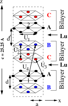
Figure 1: (Color online) Left: Fe ions in LFO. The brackets indicate a bilayer consisting of two Fe RLL’s. The presence of a TLL of Lu ions between adjacent Fe bilayers is indicated. The oxygen ions (not shown) are almost uniformly distributed over the structure. The hexagonal (conventional) unit cell contains three bilayers configured so that the TLL’s are stacked in the order ABCABC (A=red, B=black, C=blue) with two sites in the rhombohedral unit cell labeled ”1” and ”2” which are related by a center of inversion symmetry. The screened Coulomb interactions $U_{n}$ used below in our calculations are indicated. $d=2.52\AA$ and $d^{\prime}=5.81\AA$.

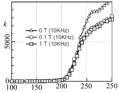
Figure 2: The dielectric constant at zero frequency from Subramanian et al[EPS, ].

As the temperature is reduced from 500K, CO correlations develop at wave vectors which nearly coincide with “root 3” (R3) ordering (see Figs. 5 and 6, below) within each TLL and eventually at the charge ordering temperature $T_{\rm CO}\approx 320$K three dimensional long range CO develops via a continuous transition.[WEN, ] Both the fluctuations and the long range order occur at incommensurate values of the wave vector.[YAMADA, ; ANGST, ] In the paraelectric phase ($T>T_{\rm CO}$) the dominant fluctuations are consistent with no enlargement of the unit cell in the ${\bf c}$ direction.[ANGST, ] We call such fluctuations “ferro-incommensurate” (FI) fluctuations to emphasize that their wave vector has incommensurate in-plane components. (The incommensurate in-plane components are very close to the values of the X point of a two dimensional triangular lattice gas with repulsive interactions, as we discuss below.) Surprisingly, the CO that occurs for $T<T_{\rm CO}$ involves a doubling of the unit cell along ${\bf c}$.[ANGST, ; REY, ] We call this ordering “antiferro-incommensurate” (AFI). These structures are shown in Fig. 3 where, for simplicity, the small incommensurability of the wave vectors is neglected. A main objective of the present paper is to explain why the CO phase is AFI and does not reflect the dominant FI fluctuations of the paraelectric (P) phase.

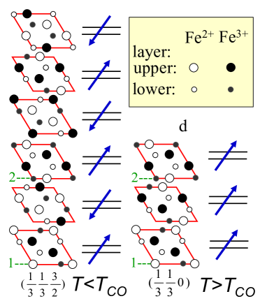
Figure 3: (Color online) From Ref. ANGST, . Fully CO structures when the incommensurability of the wave vector is neglected. The dipole moments of each bilayer (in the absence of incommensurability) as calculated in Ref. ANGST, are shown. Left: The ‘antiferroelectric’ R3 structure. Right the “ferroelectric’ R3 structure.

We will analyze this unusual CO within the lattice gas model used by Yamada et al[YAMADA, ] which we refer to as Y. The most striking result found by Y was that even with in-plane coupling $U_{1}$ and interplane couplings $U_{2}$ and $U_{3}$, long-range order is not possible because the maximum of the wave vector dependent susceptibility occurs over an entire ‘degeneration line’ in wave vector space. This result had been known for similar spin and lattice gas models on a rhombohedral lattice from the work of Rastelli and Tassi[ENRICO1, ; ENRICO2, ] and later of Reimers and Dahn[REIMERS, ]. As Y found, it was necessary to include an interaction ($U_{4}$ in Fig. 1) between next-nearest neighboring TLL’s in order to remove this degeneracy. We will analyze this situation in detail and show that there are two crucial parameters which govern this phenomenon. The first parameter is the interaction $U_{2}$ in Fig. 1 which scales the radius of the cylinder on which the degeneration line is wrapped. The second parameter is the interaction $U_{4}$ in Fig. 1 which removes the continuous degeneracy and leads to an energy variation of amplitude $\Delta E$ as one traverses the degeneration line. To elucidate our mean-field results we will briefly review the results for a single TLL with repulsive interactions. Repulsive interactions are clearly relevant for the charge-charge interactions. For magnetic interactions the presence of many exchange paths through intervening oxygen ions suggests that the magnetic interactions should also be repulsive (i. e. antiferromagnetic). The most general result of our analysis is that the wave vector of the stacked TLL’s of LFO is unstable at X (the wave vector which characterizes the R3 structure) if a continuous transition is assumed, in which case the ordered phase must perforce be incommensurate.

This same logic applies to the magnetic phase transition into the spin ordering (SO) phase which appears at $T=240$K. We will discuss the ramifications of the fact that the magnetic transition appears to be a continuous one to a commensurately ordered spin state. We will give a Landau analysis of the symmetry of the SO phase and will discuss microscopic interactions which can explain this ordering. Finally, we will discuss briefly a possible explanation of recent field-cooled experiments[WEN, ] which show that such a protocol has seems to significantly destabilize the AFI CO state.

Below 170K the system undergoes another transition in which the magnetic order parameter sharply decreases.[CHRIST, ] The details of this state are not settled at present[WEN, ] and we will not consider it further. Thus the magnetoelectric phase diagram we are considering is that shown in Fig. 4. A brief summary of this work appeared some time ago.[PRE, ]

Figure 4: The magnetoelectric phase diagram of LFO based on the results discussed in the text.

II MEAN FIELD TREATMENT OF CO

II.1 Calculation

We start with a Landau analysis of CO using the lattice gas model of Y in which one introduces a variable $\sigma_{n}({\bf R})$, where $n$ ($n=1,2$) labels the $n$th site of the rhombohedral unit cell at ${\bf R}$. which assumes the value $+1$ ($-1$) if the site is occupied by an Fe³⁺ (Fe⁺²) ion. Then $x_{n}({\bf R})\equiv\langle\sigma_{n}({\bf R})\rangle$, where $\langle\ \ \rangle$ is a thermal average. As shown in Fig. 1, we include an interaction $U_{1}$ between nearest neighbors within the same TLL, an interaction $U_{2}$ between nearest neighbors in adjacent TLL’s within the same bilayer, an interaction $U_{3}$ between nearest neighbors in adjacent bilayers, and an interaction $U_{4}$ between nearest neighbors in second-neighboring TLL’s. As argued by Y, in view of the large dielectric constant (See Fig. 2) we prefer to use a model in which the interactions fall off rapidly with separation rather than one based on a long-ranged Coulomb interaction[NAGPRL, ]. The free energy is written in terms of the Fourier transformed variables

$$x_{n}({\bf q}) = \sum_{\bf R}x_{n}({\bf R})\exp(i{\bf q}\cdot{\bf R})\ .$$ (1)

Then

$$F = \frac{1}{2}\sum_{\bf q}\sum_{n,m=1}^{2}F_{nm}({\bf q})x_{n}({\bf q})^{*}x_{m}({\bf q})+{\cal O}(x^{4})\ ,$$ (2)

where $F_{nm}({\bf q})=F_{mn}({\bf q})^{*}$. The free energy must be invariant under spatial inversion ${\cal I}$, since ${\cal I}$ is a symmetry of this lattice. Under spatial inversion ${\cal I}$, site #1 goes into site #2, so that ${\cal I}S_{1}({\bf q})=S_{2}({\bf q})^{*}$, from which we conclude that $F_{11}=F_{22}$. A continuous CO transition is signaled by the appearance of a zero eigenvalue of the quadratic form. This instability will first occur at a wave vector whose value we wish to determine.

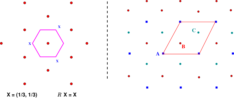
Figure 5: (Color online) Left: The reciprocal lattice of the TLL. The X points all equivalent to one another under a three-fold rotation ${\bf R}$, as discussed in the text. Right: the R3 structure associated with the wave vector of the X point. The amplitudes $Z$ of the three sites within the R3 unit cell are given by $Z_{A}=Z\cos(\phi)$, $Z_{B}=Z\cos(\phi+2\pi/3)$, and $Z_{C}=Z\cos(\phi+4\pi/3)$. The choice $\phi=0$ yields $(Z_{A},Z_{B},Z_{C})\propto(2,-1,-1)$ and the choice $\phi=\pi/6$ yields $(Z_{A},Z_{B},Z_{C})\propto(1,0,-1)$.

Figure 6: (Color online) The reciprocal lattice of the rhombohedral lattice.

Before analyzing the model in detail we review some results for the simpler problem of a lattice gas with repulsive interactions on a single TLL. In left panel of Fig. 5 we show the first Brillouin zone for the TLL with the X points which are the wave vectors of the ordered phase of this system. Note that the X point (which gives rise to the CO or SO structure, shown in the right panel of Fig. 5), is an isolated point having higher symmetry than that of all surrounding points. To see this, note that uniquely this point is invariant under a three-fold rotation about the center of zone, because under the three-fold rotation such a point is taken into another X point which is equal (modulo a reciprocal lattice vector) to to the original point. As a consequence of the special symmetry of the $X$ point, its wave vector, determined by the instability in the quadratic term of the free energy, is stable with respect to the addition of small further neighbor interactions.[STOKES, ] Such structures have been observed many times over the last half century.[GRAFOIL, ] In contrast, consider the analogous X points in the rhombohedral reciprocal lattice shown in Fig. 6. (We label these points as X regardless of the value of $q_{z}$ and refer to them as an “X line.”) Here, an X point is not invariant under a threefold rotation because the points before and after such a rotation are not equal modulo a reciprocal lattice vector. (The point is that the rhombohedral reciprocal lattice vector does not connect points before and after a three-fold rotation because the reciprocal lattice vector needed to relate the components in the plane does not have $q_{z}=0$.) So if a transition at this wave vector is continuous, the wave vector must perforce be incommensurate. Thus, without any calculation, we have shown that Landau theory explains why the CO wave vector is incommensurate. (How this conclusion relates to representation theory is discussed in Appendix A.) Accordingly, the CO phase should not display a spontaneous polarization, ${\bf P}$. The nonzero value of ${\bf P}$ may be an artifact of the small electric field applied during the experiment (as argued in Ref. ANGST, ). Also, it is possible that the pyroelectric current (from which the value of ${\bf P}$ is deduced) might be confused with currents which develop in the conductive sample.[WEN2, ] At a recent conference it was reported that ${\bf P}=0$ at low temperature. We will discuss below that a similar analysis of the magnetic phase transition at $T=240$K indicates that if that transition is continuous the ordered phase ought to be incommensurate.

We now return to the explicit calculation of the incommensurate CO wave vector. As mentioned in the introduction, from previous work [ENRICO1, ; ENRICO2, ; REIMERS, ; YAMADA, ] it is known that the minimal model that gives stable three-dimensional long-range order requires the interactions shown in Fig. 1. Other interactions (such as a second-neighbor in-plane interaction or a second neighbor interaction between adjacent TLL’s) only lead to perturbative corrections. Therefore we simplify the analysis by only considering the minimal model. To determine the wave vector of CO within this model, we analyze the appearance of a zero eigenvalue of the quadratic form of Eq. (2). In mean field theory one writes

$$F_{nm}({\bf q})=c^{\prime}kT\delta_{nm}+\sum_{\bf R}U(0,m;{\bf R},n)\exp(i{\bf q}\cdot{\bf R})\ ,$$ (3)

where $c^{\prime}$ is a constant of order unity and $U(0,m;{\bf R},n)$ is the interaction between sites $m$ in the rhombohedral unit cell at the origin and $n$ in the rhombohedral unit cell at ${\bf R}$. We set $c^{\prime}=1$, and $k_{B}=1$, and henceforth, unless stated otherwise, all energies will be in temperature units. In Cartesian coordinates

$$F_{11} = T+U_{1}[2\cos(aq_{x})+4\cos(aq_{x}/2)\cos(\sqrt{3}aq_{y}/2)]$$

$$+U_{4}\left[e^{icq_{z}/3}\Lambda(q_{x},q_{y})+e^{-icq_{z}/3}\Lambda(q_{x},q_{y})^{*}\right]$$

$$F_{21} = U_{2}e^{-2icq_{z}/3}\Lambda(q_{x},q_{y})+U_{3}e^{-icq_{z}/3}\Lambda(q_{x},q_{y})^{*}\ ,$$ (4)

where

$$\Lambda(q_{x},q_{y}) = 2e^{iq_{y}a\sqrt{3}/6}\cos(aq_{x}/2)+e^{-iaq_{y}\sqrt{3}/3}\ .$$ (5)

To organize the calculation we will consider $U_{n}/U_{1}$ for $n>1$ to be of order the expansion parameter $\lambda$ and we will work consistently to the lowest sensible order in $\lambda$, keeping in mind that for $U_{4}=0$ we have a line of infinite degeneration[YAMADA, ; ENRICO1, ; ENRICO2, ; REIMERS, ]. In any event these works indicate that for $U_{1}>0$ the instability in the quadratic form first appears near the $X$ point, for some discrete values of $q_{z}$, for $U_{4}\not=0$ and for all $q_{z}$ for $U_{4}=0$. Accordingly, we set $aq_{x}=4\pi/3+\rho_{x}$ and $aq_{y}=\rho_{y}$ and determine $\rho$ to leading order in $\lambda$ for arbitrary $q_{z}$.

For this purpose we evaluate the matrix $F_{nm}$. We find that up to order $U_{1}\lambda^{2}$,

$$F_{11} = T+U_{1}[-3+(3/4)\rho^{2}]-U_{4}\sqrt{3}\rho\cos(\phi+ck_{z}/3)\ ,$$ (6)

where $\rho\cos\phi=\rho_{x}$ and $\rho\sin\phi=\rho_{y}$, with $\rho>0$, and $\rho^{2}=\rho_{x}^{2}+\rho_{y}^{2}$. As we shall see below, $\rho={\cal O}(\lambda)$ and to clarify the situation it is only necessary to calculate the eigenvalues of the quadratic form ${\bf F}$ to order $\lambda^{2}U_{1}$.

$$\Lambda=-(\sqrt{3}/2)\rho e^{i\phi}\ .$$ (7)

Thus the critical eigenvalue, $\mu({\bf q})$ which first approaches zero as the transition is approached is given by $F_{11}-|F_{12}|$ or, up to order $U_{1}\lambda^{2}$,

$$\mu({\bf q}) = T+U_{1}[-3+(3/4)\rho^{2}]-U_{4}\sqrt{3}\rho\cos(\phi+cq_{z}/3)$$ (8)

$$-\frac{\sqrt{3}\rho}{2}\Bigl{[}U_{2}^{2}+U_{3}^{2}+2U_{2}U_{3}\cos(2\phi-cq_{z}/3)\Bigr{]}^{1/2}\ .$$

Note that for a single TLL, for which $U_{2}=U_{3}=U_{4}=0$ the X point with $\rho=0$ is stable and that, in view of the term linear in $\rho$, the X point becomes unstable in the presence of interlayer interactions.[LAMBDA, ] One might have expected to have three dimensional long-range order when $U_{1}$, $U_{2}$, and $U_{3}$ are all nonzero because then each TLL’s interacts with ones above and below it. However, the special symmetry of the rhombohedral lattice prevents ordering[ENRICO1, ; ENRICO2, ; REIMERS, ; YAMADA, ] when only these interactions are present, so we are forced to include a nonzero value of $U_{4}$.

We first minimize $\mu({\bf q})$ with respect to $\rho$, which is determined by

$$0 = \frac{\partial\mu}{\partial\rho}=-\sqrt{3}U_{4}\cos(\phi+cq_{z}/3)+\frac{3}{2}U_{1}\rho-\frac{\sqrt{3}}{2}[U_{2}^{2}+U_{3}^{2}+2U_{2}U_{3}\cos(2\phi-cq_{z}/3)]\ .$$ (9)

Thus the value of $\rho$ which minimizes $\mu$ and which we denote $\rho^{*}$ is given by

$$\rho^{*} = (2\sqrt{3}/3)(U_{4}/U_{1})\cos(\phi+cq_{z}/3)$$ (10)

$$+\frac{\sqrt{3}}{3U_{1}}[U_{2}^{2}+U_{3}^{2}+2U_{2}U_{3}\cos(2\phi-cq_{z}/3)]\ .$$

As we mentioned, $\rho^{*}$ becomes nonzero at order $\lambda$. Since $\partial\mu/\partial\rho=0$ at the extremum, corrections to $\rho^{*}$ at the next order in $\lambda$ do not affect the result we find for the critical eigenvalue $\mu(q_{z},\phi,\rho^{*}(q_{z},\phi))$:

$$\mu(q_{z},\phi) = T-3U_{1}-\sqrt{3}\rho^{*}U_{4}\cos(\phi+cq_{z}/3)+(3/4)U_{1}(\rho^{*})^{2}$$ (11)

$$-(\sqrt{3}\rho^{*}/2)[U_{2}^{2}+U_{3}^{2}+2U_{2}U_{3}\cos(2\phi-cq_{z}/3)]^{1/2}$$

$$= T-3U_{1}-(U_{4}^{2}/U_{1})\cos^{2}(\phi_{+})-(U_{4}X/U_{1})\cos(\phi_{+})-X^{2}/(4U_{1})\ ,$$

where $\phi_{+}=\phi+ck_{z}/3$ and

$$X = \left[U_{2}^{2}+U_{3}^{2}+2U_{2}U_{3}\cos(2\phi-cq_{z}/3)\right]^{1/2}\ .$$ (12)

When $U_{4}=0$, the critical eigenvalue is a function of the variable $2\phi-cq_{z}/3$ and the eigenvalue is minimal for $2\phi-cq_{z}/3=0$ or $2\pi$ if $U_{2}U_{3}>0$ and for $2\phi-cq_{z}/3=\pi$ or $-\pi$ if $U_{2}U_{3}<0$, consistent with the results cited for the line of degeneration.

The values of $\phi$ and $cq_{z}$ which complete the determination of the critical wave vector when $U_{4}\not=0$ are selected as those which minimize $\mu$. If we define

$$n \equiv U_{4}/|U_{4}|\ ,\hskip 72.26999ptm\equiv U_{2}U_{3}/|U_{2}U_{3}|\ ,$$ (13)

then we see that $\mu$ is minimized by setting

$$\cos(\phi+cq_{z}/3)=n\ ,\hskip 72.26999pt\cos(2\phi-cq_{z}/3)=m\ ,$$ (14)

so that

$$\phi+cq_{z}/3 = (1-n)\pi/2+2k\pi\ ,\hskip 72.26999pt2\phi-cq_{z}/3=(1-m)\pi/2+2l\pi\ ,$$ (15)

where the integers $k$ and $l$ are free parameters. We therefore get the results of Table 1, shown in Figs. 7-10.

Table 1: The critical wave vector as a function of the $U$’s is given by $\vec{q}=(\rho\cos\phi,\rho\sin phi,q_{z})$, where $\rho$ is given by Eq. (10) and $\phi$ and $q_{z}$ are given below, where $p$ is an integer.

$\frac{U_{2}U_{3}}{|U_{2}U_{3}|}$	$\frac{U_{4}}{|U_{4}|}$	$\phi$	$cq_{z}$
+	+	$\frac{2p\pi}{3}$	$-2p\pi$
+	-	$\frac{(2p+1)\pi}{3}$	$2\pi(-p+1)$
-	+	$\frac{(2p+1)\pi}{3}$	$2\pi(-p-1/2)$
-	-	$\frac{2\pi(p+1)}{3}$	$2\pi(-p+1/2)$

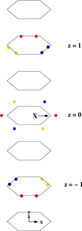
Figure 7: (Color online) Scattering for positive $U_{2}U_{3}$ and positive $U_{4}$. The $x$ and $y$ axes of the scattering vector $\vec{q}$ are indicated. Its $z$-component is $q_{z}=2\pi z/c$. The $X$ point, which in hexagonal notation is $(1/3,1/3,0)$, is indicated. Here we show the diffuse scattering in the charge disordered phase (where the colors have no significance.) If the system were to order, one would have Bragg scattering from each of the three domains. The scattering from a single domain is indicated by a single color (red, blue, or gold). Note that the diffuse scattering exhibits all the symmetries of the crystal, whereas a single domain has lower symmetry, since it does not have three fold symmetry. However, if all domains are equally populated, then the three fold symmetry is restored. This is the result for the crystal shown in Fig. 1. Note that the mirror which takes $y$ into $-y$ is not a symmetry of the crystal and it leads to a slightly different diffraction pattern.

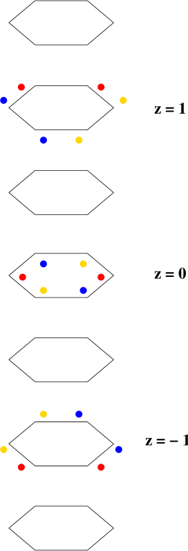
Figure 8: (Color online) As Fig. 7, but for positive $U_{2}U_{3}$ and negative $U_{4}$.

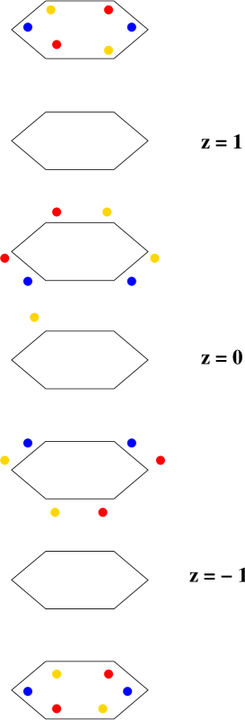
Figure 9: (Color online) As Fig. 7, but for negative $U_{2}U_{3}$ and positive $U_{4}$.

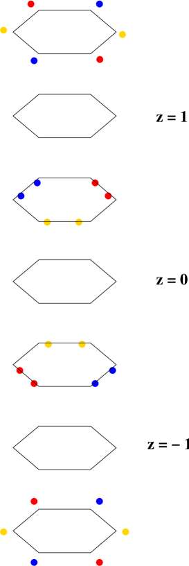
Figure 10: (Color online) As Fig. 7, but for negative $U_{2}U_{3}$ and negative $U_{4}$.

II.2 Comparison to Experiment

Now we compare these results with experiment and if we obtain agreement we should be able to identify some of the parameters. Look at the data shown in Fig. 11. Note that the diffraction pattern at $l=15$ (or $l=18$) can be compared with that for $l=0$ in Figs. 7 to 10. Note that the data indicate that the diffraction at $l=15$ occurs for $\phi=\pi$ [since it is closer to $(0,0,l)$ than is the commensurate location]. So this is the same as shown in Fig. 8 for $U_{2}U_{3}>0$ and $U_{4}<0$ and can also be confirmed by comparison with that case (for $p=1$) in Table I. Furthermore, as one moves in the direction of positive $l=q_{z}$, one sees that $d\phi/dl=-2\pi/3$ in both the experiment and in Fig. 8. (Although this line shows a definite sign of helicity, the system as a whole is not chiral. Of the six lines equivalent to the one shown in Fig. 11, three of them have one sign of helicity and three the other sign of helicity.) We can also check that our eigenvector of the matrix $\bf F$ of Eq. (2) agrees with that used in Ref. ANGST, . They use $[1,-1]$ for FI ($l=0$) diffraction (see the first paragraph of p3). For us to obtain that result $F_{12}$ must be real positive (to give a minimal eigenvalue). This implies that $\phi=\pi$ which agrees with Table I. It is more problematic to connect the AFI diffraction to our analysis because the AFI phase can not be explained by the present theory, although the AFI diffraction is that shown in Fig. 10.

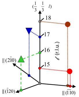
Figure 11: (Color online) From Ref. ANGST, . Diffraction maxima in the charge disordered phase ($T=360$K) near an X line. Hexagonal coordinates are used. Different colors correspond to wave vectors of different domains when CO occurs.

Now we fix the parameters to fit the existing data. In this connection we will assume that $U_{1}\gg U_{2}\gg U_{3}\gg U_{4}$, as will be justified a posteriori. Then the mean-field value of the CO transition temperature, which we denote $T_{\rm CO,MF}$ is determined by setting $\mu({\bf q})=0$. Since we believe that the heavily screened interactions decay rapidly with distance, this condition gives

$$T_{\rm CO,MF}=3U_{1}\ .$$ (16)

If we were to identify this with the observed CO transition at $T_{\rm CO}=320$K, then we would conclude that $U_{1}=110$ K. But since the coupling between bilayers is very weak, the two dimensional fluctuations will cause the observed value of $T_{\rm CO}$ to be very much less than $T_{\rm CO,MF}$. Accordingly we adopt the estimate[rho2, ]

$$U_{1} = 500{\rm K}\ .$$ (17)

Next, we have to decide whether to take $U_{2}U_{3}$ to be positive, as suggested by the fact that the P phase diffraction dominantly occurs at integer values of $cq_{z}/(2\pi)$[ANGST, ] or to be negative, as suggested by the fact that the CO phase diffraction occurs at half-integer values of $cq_{z}/(2\pi)$.[ANGST, ; IKEDA2, ; YAMADA, ] Since the corrections to our mean field theory are smallest in the P phase, we use the P phase data to fix $U_{2}U_{3}>0$ and hope to explain the CO data by some correction to this theory. (Of course, in addition, if we took $U_{2}U_{3}<0$, we would have to explain why screening causes $U_{2}$ or $U_{3}$ to be negative.) Equation (10) gives[rho, ]

$$U_{2}=\sqrt{3}\rho U_{1}=0.06U_{1}=30{\rm K}\ .$$ (18)

In view of the large ratio $U_{1}/U_{2}=15$, it seems reasonable to get $U_{2}$ under the assumption that $U_{3}/U_{2}\ll 1$. We do not have an unambiguous way to determine $U_{3}$ and $U_{4}$. However, considering that $U_{2}/U_{1}$ is about 15, we guess that $U_{2}/U_{4}=15$, which would indicate that $|U_{4}|=2$K. Previously we determined that to fit the diffraction at $T=360$K we needed to assume that $U_{4}$ was negative, so we set

$$U_{4}=-2{\rm K}\ .$$ (19)

II.3 FI versus AFI Transition Temperatures

Now we want to estimate the difference between the mean-field values of the transition temperatures for FI and AFI CO which we denote respectively as $T_{\rm MF,F}$ and $T_{\rm MF,AF}$. (By our choice of parameters $\Delta T\equiv T_{\rm MF,F}-T_{\rm MF,AF}$ is positive, which does not agree with the experimental value. We have that

$$\Delta T = \mu(cq_{z}/\pi)-\mu(cq_{z}=0)\ ,$$ (20)

when these $\mu$’s have each been minimized with respect to $\phi$ and $\rho$. Accordingly we need

$$0 = \frac{\partial\mu(\phi,q_{z})}{\partial\phi}=\frac{2U_{4}^{2}}{U_{1}}\cos(\phi_{+})\sin(\phi_{+})+\frac{U_{4}X}{U_{1}}\sin(\phi_{+})$$ (21)

$$+\frac{U_{2}U_{3}}{2XU_{1}}[X+2U_{4}\cos(\phi_{+})]\sin(2\phi-cq_{z}/3)$$

For $cq_{z}=0$, this minimization gives $\phi=\pi$, so that

$$\mu(cq_{z}=0) = T-3U_{1}-U_{4}^{2}/U_{1}+U_{4}(U_{2}+U_{3})/U_{1}-(U_{2}+U_{3})^{2}/(4U_{1})\ .$$ (22)

Now we analyze the extremum of $\mu$ for $cq_{z}=\pi$. All terms in Eq. (21) are of order $\lambda^{2}U_{1}$. So we assume that $U_{4}/U_{2}$ and $U_{4}/U_{3}$ are small and work to first order in those quantities. We then find that Eq. (21) yields that the extremum occurs for $\phi=\phi^{*}$, where

$$\phi^{*} = \frac{\pi}{6}-\frac{U_{4}}{U_{3}}\equiv\frac{\pi}{6}+\delta\phi\ .$$ (23)

Then

$$\mu(cq_{z}=\pi) = T-3U_{1}-\frac{(U_{2}+U_{3})^{2}}{4U_{1}}+{\cal O}(U_{4}^{2})$$ (24)

and

$$\Delta T = \frac{U_{4}^{2}}{U_{1}}-\frac{U_{4}}{U_{1}}(U_{2}+U_{3})\rightarrow-\frac{U_{2}U_{4}}{U_{1}}\ .$$ (25)

Note that the implied negative sign for $U_{4}$ is crucial to explain the dominance of FI fluctuations for $T>T_{\rm CO}$. Using our admittedly arbitrary estimate of $U_{4}$ we have

$$\Delta T = -\frac{U_{4}U_{2}}{U_{1}}=-\frac{(-2)(30)}{500}=0.12{\rm K}\ .$$ (26)

In view of the effect of large two dimensional fluctuations we estimate that more realistically this model would give

$$\Delta T = 0.04K\ .$$ (27)

Of course, experiment[ANGST, ] tells us that $\Delta T<0$ (i. e. the first criticality we encounter as the temperature is lowered is that toward the AFI phase) and below we will explain how this can happen, even though $U_{2}U_{3}>0$.

II.4 Summary

Note that we used the amplitude $\rho$ of the incommensurate wave vector to fix $U_{2}$, in contrast to the work of Y, who somehow uses this data to fix $U_{4}$. As we have said, the effect of $U_{4}$ is to scale the amplitude of variation of the free energy as one traverses what, when $U_{4}$ is zero, would be the degeneration line. In other words, $U_{4}$ scales $\Delta T$, the difference in the critical temperatures for FI and AFI fluctuations and the negative sign of $U_{4}$ is crucial. We find that $\Delta T$ is extremely small because it is scaled by the long range interaction $U_{4}$ between second neighboring TLL’s.

III COMPETITION BETWEEN FI AND AFI STATES

We now analyze the competition between FI ordering (at $q_{z}=0)$ and AFI ordering (at $q_{z}=3\pi/c$). Although the mean field value of the transition temperature depends only very weakly on $q_{z}$, it is simplest to invoke a model in which only FI fluctuations at $\tilde{q}_{z}=0$ and AFI fluctuations at $\tilde{q}_{z}=1/2$ compete. Therefore we are led to consider the model free energy of the form[BRUCE, ]

$$F_{0} = \frac{1}{2}(T-T_{0}+\Delta/2)x_{A}^{2}+\frac{1}{2}(T-T_{0}-\Delta/2)x_{F}^{2}+u[x_{A}^{2}+x_{F}^{2}]^{2}+vx_{A}^{2}x_{F}^{2}\ ,$$ (28)

where $x_{A}$ ($x_{F}$) is the AFI (FI) order parameter. The mean-field temperature for AFI (FI) ordering is $T_{0}-\Delta/2$ ($T_{0}+\Delta/2$) and $\Delta$ is positive for $U_{4}<0$. Then if, as is usually the case, $\Delta$ is temperature independent, one would predict that as the temperature is reduced, one would first enter the FI phase, which is not what we want. So we propose a mechanism such that $\Delta$ is temperature-dependent, so that as the temperature is decreased, we follow the dashed trajectory on the phase diagram for this model[BRUCE, ] shown in Fig. 12. There is no reason to expect that within the models considered thus far that $\Delta$ (which arose from the value of $U_{4}$) should have a relatively strong temperature dependence.[EXPL, ] It is known[RG, ] that the terms of order $x^{4}$ in Eq. (28) implement the fixed length constraint on the variables and lead to a temperature dependent renormalization of the coefficients of the quadratic terms. But there is no reason to think that such a renormalization will affect the AFI order parameter much more than the FI order parameter. It has been suggested [XU, ] that this anomalous crossover from FI to AFI fluctuations could be explained by “order from disorder.”[JV, ] Here this mechanism (of Ref. NAGPRL, ) relies on orbital fluctuations. However, it would seem that the spin-orbit interaction would cause the orbital degrees of freedom to be locked to whatever ordering occurs in the spin degrees of freedom. So we do not consider this mechanism. While it is true that at zero temperature quantum fluctuations exist in an antiferromagnet[SHENDER, ] but are zero for a ferromagnet, we are too far from that regime to invoke quantum fluctuations. Similar effects do arise from thermal fluctuations.[JV, ] But here the antiferromagnetic spin-wave energy is linear whereas the ferromagnetic spin-wave energy is quadratic in wave vector. Therefore for identical coupling constants, ferromagnetic fluctuations have lower energy than their antiferromagnetic counterparts. This argument suggests that FI fluctuations should be stronger than AFI fluctuations. Therefore we reject the suggestion[XU, ] that the cross over from FI to AFI fluctuations can be attributed to this mechanism, known as “order from disorder.”

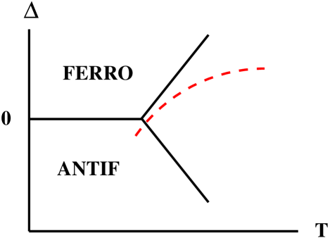
Figure 12: (Color online) Mean-field phase diagram[BRUCE, ] near the bicritical point of Eq. (28) for $v>0$. Since the dashed trajectory in the disordered (P) phase is closer to the FI phase than to the AFI phase, FI fluctuations dominate AFI fluctuations in the P phase.

Instead, to obtain the proposed trajectory shown in Fig. 12 we invoke the coupling of the FI and AFI variables to a noncritical variable, $Y$, so that the free energy is now $F=F_{0}+V$, where[FN3, ]

$$V = a|x^{2}|Y+(1/2)\chi_{Y}^{-1}Y^{2}\ ,$$ (29)

where here $x$ denotes either the FI or AFI order parameter. Also $a$ is a temperature independent coupling constant and $\chi_{Y}$ is the stiffness associated with $Y$ and is almost temperature dependent because $Y$ is far from criticality. (As we shall see, a suitable choice for $Y$ is a zone-center phonon.) Since $Y$ is a noncritical variable we can eliminate it by minimizing $F$ with respect to it, in which case we obtain

$$F = F_{0}-(1/2)\chi_{Y}a^{2}|x^{2}|^{2}\ .$$ (30)

To leading order in the fluctuations we replace $|x^{2}|^{2}\equiv{x({\bf q})^{*}}^{2}x({\bf q})^{2}$ by $4x({\bf q})x({\bf q})^{*}\langle x({\bf q})x({\bf q})^{*}\rangle$, where $\langle Z\rangle$ is the thermal expectation value of $Z$.[RG, ] Then, if the coupling constant for $FI$ fluctuations is $a_{FI}$ and that for AFI fluctuations is $a_{AFI}$, this mechanism leads to the result

$$\Delta(T)=\Delta-[a_{AFI}^{2}-a_{FI}^{2}]\chi_{Y}\langle x({\bf q})x({\bf q})^{*}\rangle\ ,$$ (31)

where we assume the thermal average is the same for FI and AFI fluctuations. So, if $a_{FI}\ll a_{AFI}$, then this mechanism leads to a renormalization of the quadratic term which is stronger for the AFI fluctuations than for the FI fluctuations. Then the natural temperature dependence of the thermal average of $|\sigma^{2}|$ can give the trajectory we desire.

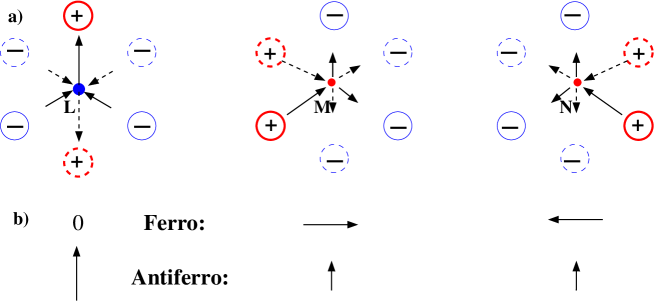
Figure 13: (Color online) a) The in-plane components of forces on sites L, M, and N in TLL₀ (as in Fig. 1) in the F configuration. The solid line vector forces are from the charges (solid circles) in the TLL above TLL₀ and the dashed line vector forces are from the charges (dashed circles) in the TLL below TLL₀. The charges at L, M, and N are negative, positive, and positive, respectively. (Red = positive, blue = negative.) The larger dots and heavier lined circles are charges of twice the magnitude of the smaller dots and lighter lined circles. b) The net force on the sites assuming the separations between all planes are the same. For the AF configuration the dashed forces are reversed and the resulting total forces are listed as “Antiferro:”. The forces are nonzero at zero wave vector only for AF ordering.

If we choose $Y$ to be a zone-center phonon, the interaction we consider is written schematically as

$$V = \frac{1}{2}\sum_{i}M\omega_{D}u_{i}^{2}+\sum_{ij}u_{ji}\cdot\Bigl{[}\nabla_{r}U(r_{ij})Q_{i}Q_{j}\Bigr{]}\ ,$$ (32)

where $M\omega_{D}$ defines the Debye model, $u$ is a phonon displacement, $U(r_{ij})$ is the heavily screened interaction, and $Q_{i}$ is the charge on site $i$. The factor in Eq. (32) in square brackets is the force on site $i$ due to the charge on site $j$.

Since we will need the phonon energies, we implemented a a first-principles calculation of the energies of the zone-center phonons in LuFe₂O₄. The calculations were performed within the plane-wave implementation of the local density approximation to density functional theory as implemented in the PWscf package.[Baroni:1, ] We used Vanderbilt-type ultrasoft potentials with Perdew-Zunger exchange correlation. A cutoff energy of 408 eV and a 9$\times$9$\times$9 k-point mesh were found to be enough for the total energy to converge within 0.5meV/atom. The gamma phonon energies were calculated using the supercell method with finite difference.[TY, ] The primitive cell was used and the full dynamical matrix was obtained from a total of eight symmetry-independent atomic displacements ($\pm$0.02 Å).

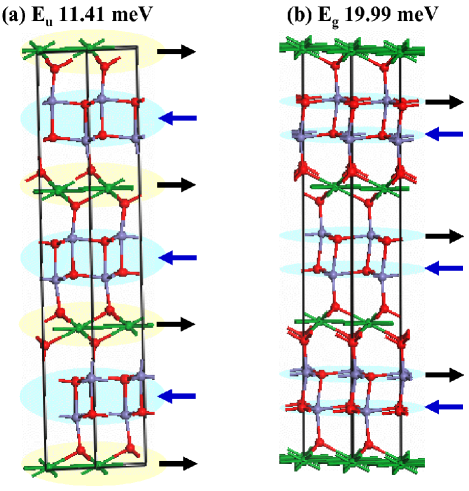
Figure 14: (Color online) The displacements of the two lowest energy modes as discussed in the text. Here O ions are red, Fe ions are purple, and Lu ions are green. The light blue ovals indicate units which move approximately rigidly.

The primitive cell contains one formula unit of LuFe₂O₄, giving rise to a total of 21 phonon branches. The phonon modes at $\Gamma$ are classified as $\Gamma$ (q=0) = 4$A_{2u}$(IR) + 3$A_{1g}$(R) + 4$E_{u}$(IR) + 3$E_{g}$(R), where R and IR correspond to Raman- and infrared-active, respectively. The nondegenerate (A) and doubly degenerate (E) modes correspond to motion along the c-axis and within the ab-plane, respectively. In the Raman-active modes the atoms at $(0,0,z)$ and $(0,0,-z)$ move out-of-phase (i.e. opposite) while in the IR-modes they move in phase.

The calculated mode energies and their symmetry labels are listed in Table 2. We hope that our calculations will initiate more experimental work such as Raman/IR measurements to confirm the $\Gamma$ phonon energies that we calculated here. From this table we see that the characteristic phonon energies are of the order of 50 or more meV. Since the coupling to the phonons with the lowest energies will be the most effective, we show the two lowest energy phonons schematically in Fig. 14.

The lowest energy mode with E_u symmetry and 11.4 meV energy corresponds to displacements in the ab plane in which the LuO and FeO-bilayer move in opposite directions as rigid units (see Fig. 14a). Hence the energy of this mode is basically determined by the strength of LuO-Fe-O bond angle. Even though this mode has the lowest energy, its symmetry is not right to create the electrostatic forces needed for our mechanism. The next mode has the E_g symmetry and it corresponds to displacements in the ab-plane (Fig. 14b) in which the two TTL’s of each bilayer moves in opposite directions while LuO-layer is fixed. Hence this modes involves twice as much O-Fe-O bond bending as the lowest energy mode and interestingly it has about the twice energy (20 meV) of the E_u mode shown in Fig. 14a. As we shall see, it is this mode that creates the electrostatic forces needed for our mechanism.

Table 2: List of phonon symmetries and calculated energies (in meV) of LuFe₂O₄ at the $\Gamma$ point of the primitive cell, as obtained from the first-principles calculations described in the text.

Mode Symmety	Eu	Eg	A2u	A1g	A2u	Eu
Energy (meV)	11.41	19.99	20.02	31.48	38.46	41.20
Mode Symmety	A1g	Eg	A2u	Eu	Eg	A1g
Energy (meV)	53.25	54.73	57.69	58.79	62.62	84.96

Accordingly, we look for charge-phonon interactions which involve zone-center transverse (to the $c$-axis) phonons. We now analyze the force on the Fe charges in a given TLL, which we denote TLL₀, from the nearest neighboring Fe TLL’s above and below TLL₀. Since we consider coupling to the lowest energy phonons, which involve motion transverse to the ${\bf c}$ axis, we will only consider forces in the plane of the TLL. Phonon modes which decrease the distance between TLL’s will involve higher energy. One sees that a low energy mode which can couple the way we want is a zone-center phonon in which alternate TLL’s are displaced transversely relative to one another. For this rhombohedral lattice, such a mode is an E_g mode. As mentioned this is the E_g mode at 19.99 meV. To see whether this mode couples differently to FI and AFI fluctuations, we have only to analyze the transverse force on one TLL from the TLL’s above and below it. Since we are near the transition, we assume the R3 structure of the fluctuations (see Fig. 5, where we choose $\phi=0$) and add up the forces in Fig. 13. Also, we simplify the argument by neglecting the fact that the interlayer separation is different for TLL’s within the same bilayer and for TLL’s in adjacent bilayers.

We now estimate quantitatively the effect of this coupling in Eq. (32). As in Fig. 1, the $Q$’s are given in terms of the order parameter $x_{\rm X}$, where $X$ indicates either the FI or AFI configuration of TLL’s. Because the transverse motion of planes is relatively soft, we consider displacements to lie within the TLL₀ plane. When minimized with respect to $u_{i}$, the free energy is

$$F_{\rm Ph} = -\frac{z_{X}^{2}|x_{X}|^{4}}{2M\omega_{D}^{2}}\left(\frac{U}{r}\right)^{2}\left(\frac{r_{\parallel}}{r}\right)^{2}\xi^{2}\ ,$$ (33)

where $\xi=(r/U)(dU/dr)$, $r_{\parallel}$ is the component of $r$ within the TLL, and $z$ is the effective number of nearest neighbors. Also we set $U=(U_{2}+U_{3})/2=16.5$K $\approx$ 1.5 meV. The actual number of nearest neighbors is 6, but since the forces do not all add up, we take $z=3$ for the AF configuration and $z=0$ for the F configuration where the forces from adjacent TLL’s nearly cancel. We set $\hbar\omega_{D}=20$ meV, $r=5\AA$, and $r_{\parallel}=2\AA$. The factor $\xi$ depends on how rapidly the interaction decreases with distance. For bare Coulomb interactions $\xi=-1$. But we are far from that regime. We take $\xi=-10$, which is a value often found for exchange interactions in insulators.[BLOCH, ] Also the Fe mass is $M=60$ amu, so its reduced mass is 30 amu. Thus

$$F_{\rm Ph} = -F_{0}|x_{\rm AF}^{4}|\rightarrow-\frac{1}{2}\Bigl{(}8F_{0}\langle|x_{\rm AF}|^{2}\rangle\Bigr{)}|x_{\rm AF}|^{2}\ ,$$ (34)

where $F_{0}\approx 0.004$meV. Then identifying $(8F_{0}\langle|x_{\rm AF}|^{2}\rangle)$ as the renormalization of $T_{\rm CO}$ we get

$$\Delta(T)\approx\Delta-0.032{\rm meV}\langle|x_{\rm AF}^{2}|\rangle\approx 0.04{\rm K}-(0.4{\rm K})\langle|x_{\rm AF}^{2}|\rangle\ .$$ (35)

which is enough to shift ordering from F to AF at $T_{\rm CO}$, where $\langle|x_{\rm AF}^{2}|\rangle\approx 1/2$.

Finally, we should mention that this frozen phonon occurs whether or not the CO phase is commensurate because its origin is in a coupling of the form

$$V\sim u({\bf q}=0)\sigma({\bf q})\sigma(-{\bf q})\ ,$$ (36)

where $\sigma({\bf q})$ is the CO order parameter.

IV The Magnetic Phase Transition

IV.1 Phase of the R3 Structure

We now discuss the magnetic phase transition at which SO appears. At first we neglect the fact that the system is a mixture of spins of magnitude 2 and spins of magnitude 5/2 and we assume that the uniaxial anisotropy aligns the spins along the ${\bf c}$ axis. Then one introduces the local order parameter $S({\bf r})$ as the thermal average of $S_{z}({\bf r})$, the $z$-component of spin at the site ${\bf r}$. Also, as noted in Ref. CHRIST, , if one neglects the coupling between spin and charge, the symmetry of the SO free energy is the same that of the CO free energy of Eq. (2). Thus, if the transition is assumed to be continuous, the ordering wave vector for this transition should be unstable relative to the X point, just as we argued (in connection with Fig. 6) in the case of the CO transition. In that case the representation analysis of Ref. CHRIST, for the wave vector $(1/3,1/3,0)$ is not definitive. However, we temporarily overlook the possible instability of the X wave vector and apply Landau theory to the phase transition as if this wave vector were stable. (In Appendix A we discuss some difficulties in applying representation analysis to this transition.) Therefore we write the free energy in terms of $S_{1}({\bf q})=S_{2}({\bf q})\equiv S({\bf q})$, where the subscript labels the two Fourier components of the unit cell. We have that

$$F=(1/2)(T-T_{SO})|S({\bf q})|^{2}+u|S({\bf q})|^{4}+v|S({\bf q})|^{6}+\dots+wS({\bf q})^{6}+w^{*}{S({\bf q})^{*}}^{6}\ ,$$ (37)

where $T_{SO}$ is the magnetic (SO) transition temperature and we will set

$$S({\bf q}) = |S({\bf q})|e^{i\phi}\ .$$ (38)

Under inversion symmetry $S({\bf q})\rightarrow S({\bf q})^{*}$, which implies that $w$ in Eq. (37) is real. The last term in Eq. (37) is the lowest order one that fixes the phase $\phi$ of the order parameter. (It should be noted that it is not easy to fix the this phase using only scattering data.) There are two cases:[RHO, ]

$$\phi=n\pi/3\ \ \ {\rm if}\ w<0\ ;\hskip 72.26999pt\phi=(n+1/2)\pi/3\ \ \ {\rm if}\ \ w>0\ ;$$ (39)

with the results for the amplitudes in the magnetic unit cell as given in the caption to Fig. 5. To determine the net moment of these structures it is necessary to analyze the admixture of wave vector $(0,0,0)$.[CERR, ] Such an admixture comes about because ${\bf q}=(1/3,1/3,0)$, is 1/3 of a reciprocal lattice vector and this fact allows an additional term, $V$, in the free energy, where

$$V = -S(0,0,0)\Bigl{[}aS(1/3,1/3,0)^{3}+a^{*}{S(1/3,1/3,0)^{*}}^{3}\Bigr{]}+\frac{1}{2}\chi^{-1}S(0,0,0)^{2}\ ,$$ (40)

where $\chi$ is a stiffness (which is nearly temperature independent) and $a$ is a constant which must be real in view of inversion symmetry. Minimizing $V$ with respect to $S(0,0,0)$ we find that

$$S(0,0,0)=a\chi[S(1/3,1/3,0)^{3}+{S(1/3,1/3,0)^{*}}^{3}].$$ (41)

If $w>0$, then Eq. (39) indicates that $S(0,0,0)$ is zero, whereas for $w<0$ the system has a nonzero net moment, $M$. The early data of Ref. IIDA, suggests that $M$ is nonzero. However, recently we have learned[PC1, ] that the system is more likely to have $M=0$, in which case we must choose $w>0$. In this case one of the three sublattices is disordered. (See the caption to Fig. 5 with $\phi=\pi/6$.) In this structure, all spins within a plane perpendicular to the ordering wave vector have the same value, $a$, $-a$, or 0. This type of partial ordering was observed in the orientational ordering of solid methane[PRESS, ], and, as in that case, we would not expect a phase with partial disorder to continue to exist to arbitrarily low temperature. In Appendix B we obtain $M(H)$ for this structure.

If, instead, the case $w<0$ is realized, then one would have

$$S(0,0,0)=2a\chi S(1/3,1/3,0)^{3}$$ (42)

and if

$$S(1/3,1/3,0)\equiv B\sim(T_{\rm SO}-T)^{\beta}$$ (43)

then, within mean field theory

$$S(0,0,0)\equiv A\sim(T_{\rm SO}-T)^{3\beta}\ ,$$ (44)

which gives an unusually large critical exponent for the magnetization. For liquid crystals,[AA, ] this effect has been analyzed in detail within the renormalization group. An effect similar to this has been seen for CO.[COEXP, ]

Next we discuss the magnetic eigenvector which was chosen in Ref. CHRIST, to be $[1,1]$ (to best fit the experimental data). With this choice of eigenvector the spins form planes (perpendicular to the wave vector) of spins with amplitudes proportional to $0$, $-1$, and $1$. How is this choice to be justified within Landau theory? In the ‘minimal’ model used for CO, one sees that for $\rho=0$ (the commensurate case) $F_{12}$=0 and one has isotropy in $S_{1z}$, $S_{2,z}$ space so that the eigenvector can be $[\cos\theta,\sin\theta]$ with any choice for $\theta$. One way to explain that the eigenvector is $[1,1]$ is to invoke an interaction which tends to make the two spins in the rhombohedral unit cell parallel, so that $F_{12}$ is negative real. Since the spins are aligned along ${\bf z}$, the dipole interaction could accomplish this. However, the energy $V$ of this interaction is probably too small:

$$V = -\frac{2g^{2}\mu_{B}^{2}S^{2}}{r^{3}}=-0.045{\rm K}\ ,$$ (45)

where we set $g=2$, $S=5/2$, and $r=2d^{\prime}+d=14.1\AA$ and combine with a second term for which $r=d^{\prime}+2d=11.1\AA$. Alternative mechanisms to stabilize the antiferromagnetic spin structure involve thermal fluctuations or (as we discuss below) the distortion due to the frozen E_g phonon.

Finally we discuss the diffraction at half integer values of $L$ which has a magnetic signature and which requires positing a magnetic unit cell which is doubled along the ${\bf c}$ direction. As stated in Ref. CHRIST, one can think of this additional diffraction as being due to “the charge ordering, which decorates the lattice with differing magnetic moment on the Fe²⁺ and Fe³⁺ sites…” This effect can be seen within Landau theory as follows. We introduce an additional free energy $V$ of the following form, consistent with symmetry,

$$V = -a\sum_{\bf r}x({\bf r})S_{z}({\bf r})^{2}\ ,$$ (46)

where $a$ is a constant. The effect of this term is to increase (decrease) $S_{z}({\bf r})^{2}$ when the site is occupied by an Fe³⁺ (Fe²⁺) ion. In Fourier transform language this is

$$V = -a\sum_{n;{\bf q},{\bf k}_{1},{\bf k}_{2}}x_{n}({\bf q})S_{n}({\bf k}_{1})S_{n}({\bf k}_{2})\Delta({\bf q},{\bf k}_{1},{\bf k}_{2})\ ,$$ (47)

where $\Delta$ enforces wave vector conservation modulo a reciprocal lattice vector and the subscripts label the Fe sublattices. The term we focus on here involves charge ordering, so that ${\bf q}=(1/3,1/3,1/2)+{\mbox{\boldmath{$\delta$}}}$, where $\delta$ is the incommensurability. The magnetic variables then can involve the wave vectors ${\bf k}_{1}=(1/3,1/3,-1/2)-{\mbox{\boldmath{$\delta$}}}$ and ${\bf k}_{2}=(1/3,1/3,0)$. Then we see that this interaction couples $S(1/3,1/3,0)$ and $S(1/3,1/3,-1/2)^{*}+{\mbox{\boldmath{$\delta$}}}$. Thus the critical magnetic eigenvector is a mixture of these two variables. This corresponds exactly to the idea of “decoration,” but it is hard to estimate the importance of this effect.

IV.2 Removal of Frustration

To develop further insight into this frustrated spin system, it is useful to recall the results for the magnetic structure of the rhombohedral $\beta$-phase of solid oxygen whose structure only differs from LFO in that there are no bilayers: all TLL’s are equally spaced. (For a review see Ref. REVIEW, .) A convincing theoretical analysis based on quantum spin-wave theory was given in Refs. ENRICO1, and ENRICO2, . However, when various theoretical results were experimentally tested[DUNST, ], it was not entirely clear which theoretical model was most appropriate for $\beta$-oxygen. In any event, the magnetic correlation length is so short ($5\AA$)[DUNST, ] that is seems unrealistic to speak of any long range order.

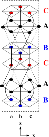
Figure 15: (Color online) Additional exchange interactions attributed to the transverse frozen phonon. Dashed (full) lines denote additional antiferromagnetic (ferromagnetic) interactions. The values of $S_{z}$ for all sites in the same $y$-$z$ plane are $a$, $b$, and $c$ as indicated, where $b=-a$ and $c=0$, in the notation of Eqs. (42) and (43). It is assumed that the in-plane interactions are dominant.

Accordingly, a central open question is to explain why the SO in LFO is so different from that of $\beta$-oxygen. One possibility is that the small distortion which we invoked to explain the crossover from FI to AFI might introduce small addition exchange interactions which remove the frustration of the rhombohedral antiferromagnet. To explore this possibility we write

$$J_{n} = J_{n}^{(0)}+\delta J_{n}\ ,$$ (48)

where the $J_{n}^{(0)}$’s are the exchange interactions which are consistent with the R$\overline{3}$m symmetry. In Fig. 15 we show a set of interactions $\delta J_{n}$ which have the correct symmetry to be induced by the frozen E_g phonon and which, if they are dominant, resolve the frustration. Note that even though CO is incommensurate, the frozen phonon is commensurate. So here we are considering a commensurate effect of incommensurate charge ordering.

To analyze this possibility, we replace the $J_{3}$ interaction by $J_{3}(1+\epsilon)$ for the dashed bonds in Fig. 15 and the other $J_{3}$ interactions by $J_{3}(1-\epsilon)$. Similarly, we replace the $J_{2}$ interaction by $J_{2}(1-\epsilon)$ for the solid bonds in Fig. 15 and the other $J_{2}$ interactions by $J_{2}(1+\epsilon)$. Then Eq. (4) remains valid but now

$$\Lambda = (1+\epsilon)e^{iaq_{y}\sqrt{3}/6}\cos(aq_{x}/2)+(1-\epsilon)e^{-iaq_{y}\sqrt{3}/3}$$ (49)

$$= -2\epsilon-(\sqrt{3}/2)(\rho_{x}+i\rho_{y})-\epsilon\rho_{x}\sqrt{3}/2+i\epsilon\rho_{y}\sqrt{3}/6+{\cal O}(\rho^{2})\ .$$

To maxmimize $|F_{21}|$ (for $U_{2}U_{3}>0$) set $\exp(icq_{z}/3)=\Lambda/\Lambda^{*}$, so that

$$|F_{21}| = (U_{2}+U_{3})|\Lambda|\ .$$ (50)

Then the minimal eigenvalue is found by minimizing

$$\mu(\rho_{x},\rho_{y}) = T-3U_{1}+(3/4)U_{1}\rho^{2}$$ (51)

$$-(U_{2}+U_{3})\Biggl{(}[2\epsilon+(1+\epsilon)(\sqrt{3}/2)\rho_{x}]^{2}+(3/4)(1-\epsilon/3)^{2}\rho_{y}^{2}\Biggr{)}^{1/2}\ .$$

When $\epsilon=0$, this is a function of $\rho_{x}^{2}+\rho_{y}^{2}$ and is consistent with the existence of a degeneration line. However, when $\epsilon$ is nonzero, then the minimum occurs for $\rho_{y}=0$ (so that $q_{z}=0$) and

$$\rho_{x} = (1+\epsilon)(U_{2}+U_{3})/(\sqrt{3}U_{1})\ .$$ (52)

One might wonder where the extrema we found for CO at $cq_{z}=2p\pi$, for $p=1$ and $p=2$ have gone. The answer is that there are three CO domains corresponding to which there are three distortions, the transverse phonon displacement being perpendicular to the in-plane projection of the ordering wave vector. So we have three different SO domains, each one tied to one of the three possible CO domains.

An important question is: since the wave vector is not at a special, high-symmetry point (see Fig. 6), the wave vector should not be commensurate if the SO transition is a continuous one. It is not clear that the sensitivity of the neutron diffraction experiment of Ref. CHRIST, is sufficient to detect the very small incommensurability that might attend this magnetic transition. It would be of interest to have a high precision determination of the SO wave vector, to check whether it is or is not commensurate.

If the SO phase is truly commensurate, then one would have to entertain a scenario to accommodate such a fact. The one scenario that is excluded is that the commensurate SO state is reached via a single continuous phase transition. Possibly there are two phase transitions, the first, in which there develops incommensurate order, followed by a second one into the commensurate antiferromagnetic state.[DS, ] The presence of two nearby transitions in parameter space would seem to signal a nearby multicritical point at which the two transitions coincide. To check for that, it would be useful to have very precise measurements of the specific heat and susceptibility to get the critical exponents that characterize this transition. A different scenario is that the magnetic transition is a first order one to a commensurate SO phase.

IV.3 Field Cooling

Finally, we mention the intriguing data of Fig. 3c of Ref. WEN, , where it is shown that cooling in a field along $(1,-1,0)$ from $T>T_{CO}$ causes a pronounced reduction in the CO diffraction at 300K. This data raises a natural unanswered question: does this ‘missing” intensity in the AFI scattering show up as new FI scattering at $(1/3,1/3,n)$ for integer $n$. If so, it would mean that the magnetic field could stabilize the FI state for $T<T_{CO}$ and it would be of interest to know whether such a state was or was not commensurate.

Here we present a partial explanation for the above field cooling scenario. We start by noting that in Ref. WEN, it is shown that application of a magnetic field in the plane of the TLL’s decreases the AFI correlation length. This suggests that such a magnetic field tends to destabilize the AFI phase, possibly making the FI phase relatively more stable. If this is the case, the one might have a phase diagram like that shown in Fig. 16. Then in the various scenarios of cooling one would start in the disordered phase at points like A and B and cool to points A’ and B’. Clearly, if this is done at zero field and then a field not large enough to go into the FI phase is applied, no dramatic field dependence will be observed, in agreement with their observations. However, if one starts from point like A or B, then when the system is cooled it passes though a region of FI ordering which then can be supercooled while reaching the final points A’ or B’. Then, as a function of time the system would evolve in some irregular process into the equilibrium state of AFI order. This might happen without displaying a dramatic dependence on the field-cooled value of the magnetic field. Indeed the data shows that after a sharp decrease for very small field, the resulting AFI order does not depend strongly on $H$. This proposal suggests that it would be useful to monitor the $(1/3,1/3,0)$ reflection under field cooled conditions (to see if the decrease in intensity at $(1/3,1/3,3/2)$ is accompanied by an increase at $(1/3,1/3,0)$. It would indeed be interesting if an in-plane magnetic field could stabilize a nonzero polarization. Note that an in-plane magnetic field may be more effective than one parallel to the $c$-axis, because the perpendicular susceptibility is usually larger than the parallel susceptibility.

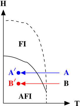
Figure 16: (Color online) Proposed phase diagram for CO as a function of maganetic field $H$ and temperature $T$. Dashed lines represent continuous transitions and the solid line a first order transition.

V SUMMARY

Here we briefly summarize our conclusions.

$\bullet$ We show that the appearance of an incommensurate wave vector for charge ordering is a result of symmetry (or more accurately, due to a lack of symmetry).

$\bullet$ By comparing our theory with experiment we have assigned values to several of the phenomenological charge-charge interactions. In particular, the signs and magnitude of the incommensuration and the fact that ferroelectric fluctuations dominate in the disordered phase are explained by simple choice of these interactions.

$\bullet$ The cross over, as the temperature is lowered through the charge ordering temperature, from ferroelectric to antiferroelectric incommensurate structure can be explained by the temperature dependent renormalization of the transition temperature due to charge-phonon coupling.

$\bullet$ We have performed a first-principles calculation of the zone center phonon energies (assuming no ordering of charge or spin). The phonon with the correct symmetry to couple effectively to the charge ordering has a rather low (20 meV) energy, corresponding to the sliding (transverse to the ${\bf c}$ axis) of alternate Fe layers with respect to one another.

$\bullet$ We have developed a Landau theory which describes the phase of the recently observed spin ordered state having zero net magnetic moment.

$\bullet$ In principle, if the spin ordering transition is continuous, the spin ordered phase would be expected to be incommensurate. This suggests the need for a high precision determination of the spin ordering wave vector to check whether it is or is not commensurate. If the spin ordered phase truly is commensurate, then it would be of interest to investigate the scenario of ordering, which can not be via a single continuous transition. One way to pin down the scenario would be to determine the critical indices $\alpha$, $\beta$, and $\gamma$, associated respectively with the specific heat, the magnetic order parameter, and the susceptibility.

$\bullet$ We have also suggested experiments to test our proposal that the sharp decrease in intensity of antiferroelectric charge scattering as a function of magnetic field in the field cooled scenario might indicate that the magnetic field tends to stabilize ferroelectric charge ordering and possibly a consequent polarization.

ACKNOWLEDGEMENTS We thank A. D. Christianson and M. Angst for helpful correspondence, and A. Boothroyd for introducing us to this subject. We also thank Q. Xu, S. Shapiro, D. Singh, E. J. Mele and T. C. Lubensky for stimulating discussions. We also thank E. Rastelli for a discussion of Refs. ENRICO1, and ENRICO2, .

Appendix A Representation Theory

In Refs. CHRIST, and ANGST, representation theory is used to analyze possible magnetic ordering patterns and charge ordering patterns, respectively. In their approach, they implicitly assume that the wave vector at the appropriate X point is stable with respect to the addition of further neighbor interactions. As we have seen in Sec. II, this assumption is not actually valid, especially for CO. To see this explicitly, consider the structure of the two by two matrix $F_{nm}$ of Eq. (4) which determines the eigenvectors. Exactly at the X point and when arbitrary interactions are allowed, $F_{21}$ is scaled by the interactions $V_{1,2}$ between sites #1 and #2 which are displaced from one another by a vector along the $c$-axis. This interaction is extremely small, since it connects sites which are not in adjacent bilayers, but are in second (or further) neighboring bilayers. Representation theory bases the eigenvector equation on this symmetry and leads to eigenvectors that are either even or odd under inversion.

However, as noted in Sec. II, this type of analysis is invalidated by the fact that for LFO the X point is not actually stable. For wave vectors near the X point, we explicitly displayed in Eq. (7) the term in $F_{12}$ which is linear in the displacement from the X point. The interactions $U_{2}$ and $U_{3}$ which scale this linear term are very much larger than $V_{1,2}$ whose existence is ignored if representation theory is invoked for the commensurate case. The major effect of this linear term is that the eigenvectors, instead of being even and odd, as in the analysis of Refs. CHRIST, and ANGST, , are now complex and are determined by the phase of $F_{21}$ given by Eqs. (4) and (7). Note that this phase will, in general, be different for each of the three domains, and inclusion of the correct phases, might affect the determination of the domain populations.

Appendix B Equation of State for the Antiferromagnet

In this appendix we obtain $M(H)$, where $M$ is the net magnetization (along the ${\bf c}$ axis) for the model of Eq. (37) and $H$ is the external field applied parallel to the $c$ axis. Accordingly we add to the free energy the term $-HM$, where $\chi$ is the parallel susceptibility, so that with $|S({\bf q})|\equiv\sigma$, we have

$$F=\frac{1}{2}(T-T_{SO})\sigma^{2}+u\sigma^{4}+4w\sigma^{6}\cos^{2}(3\phi)-2a\sigma^{3}M\cos(3\phi)+\frac{1}{2}\chi^{-1}M^{2}-MH\ ,$$ (53)

where $\chi$ is the parallel susceptiblity and we kept $\phi$-independent terms only up to order $\sigma^{4}$ because our analysis is not valid when $T\ll T_{SO}$. Minimizing with respect to $M$ yields

$$M = \chi[H+2a\sigma^{3}\cos(3\phi)]$$ (54)

so that

$$F = \frac{1}{2}(T-T_{\rm SO})\sigma^{2}+u\sigma^{4}+4w\sigma^{6}\cos^{2}(3\phi)-\frac{1}{2}\chi[H+2a\sigma^{3}\cos(3\phi)]^{2}\ .$$ (55)

When this is minimized with respect to $\phi$ we find two regimes:

$$H>H_{c}\ :\hskip 72.26999ptM = \chi\Bigl{[}H+2a\sigma^{3}\Bigr{]}$$

$$H<H_{c}\ :\hskip 72.26999ptM = \chi H\Bigl{[}1+\frac{2a^{2}\chi}{4w-2a^{2}\chi}\Bigr{]}\ ,$$ (56)

where

$$H_{c} = \frac{(4w-2a^{2}\chi)\sigma^{3}}{a\chi}\ .$$ (57)

which leads to the $M$ versus $H$ curve shown in Fig. 17. The value of $\sigma$ is approximately $[(T_{\rm SO}-T)/(4u)]^{1/2}$ for $T$ near $T_{\rm SO}$.

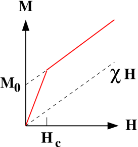
Figure 17: (Color online) The $c$-component of magnetization $M$ (solid line) versus the magnetic field $H$ along ${\bf c}$ for the antiferromagnetic phase. Here $M_{0}=2a\chi\sigma^{3}$ and $H_{c}$ is given by Eq. (57). Near $T_{\rm SO}$ both $M_{0}$ and $H_{c}$ are of order $(T_{\rm SO}-T)^{3/2}$.

References

- (1) E. J. W. Verwey, Nature 144, 327 (1939).
- (2) P. W. Anderson, Phys. Rev. 102, 1008 (1956).
- (3) J. P. Wright, J. P. Attfield, and P. G. Radaelli, Phys. Rev. B 66, 214422 (2002).
- (4) D. I. Khomskii, J. Mag. Mag. Mater. 306, 1 (2006).
- (5) J. Iida, M. Tanaka, Y. Nakagawa, S. Funahashi, N. Kimizuka, and S. Takekawa, J. Phys. Soc. Jpn, 62, 1723 (1993).
- (6) Y. Yamada, K. Kitsuda, S. Nohdo, and N. Ikeda, Phys. Rev. B 62, 12167 (2000).
- (7) N. Ikeda, K. Kohn, N. Myouga, E. Takahashi, H. Kitoh, and S. Takekawa, J. Phys. Soc. Jpn, 69, 1526 (2000).
- (8) N. Ikeda, H. Ohsumi, K. Ohwada, K. Ishii, T. Inami, K. Kakurai, Y. Murakami, K. Yoshii, S. Mori, Y. Horibe, and H. Kito, Nature 436, 1136 (2005).
- (9) M. A. Subramanian, T. He, J. Chen, N. S. Rogado, T. G. Calvarese, and A. W. Sleight, Adv. Mater. 18, 1737 (2006).
- (10) Y. Zhang, H. X. Yang, C. Ma, H. F. Tian, and J. Q. Li, Phys. Rev. Lett. 98, 247602 (2007).
- (11) A. D. Christianson, M. D. Lumsden, M. Angst, Z. Yamani, W. Tian, R. Jin, E. A. Payzant, S. E. Nagler, B. C. Sales, and D. Mandrus, Phys. Rev. Lett. 100, 107601 (2008).
- (12) M. Angst, R. P. Hermann, A. D. Christianson, M. D. Lumsden, C. Lee, M.-H. Whangbo, J.-W. Kim, P. J. Ryan, S. E. Nagler, W. Tian, R. Jin, B. C. Sales, and D. Mandrus, Phys. Rev. Lett. 101, 227601 (2008).
- (13) J. Wen, G. Xu, G. Gu, and S. M. Shapiro, Phys. Rev. B 80, 020403 (2009).
- (14) M. Isobe, N. Kimizuka, J. Iida, and S. Takekawa, Acta Cryst. C46, 1917 (1990).
- (15) A. J. C. Wilson, International Tables for Crystallography (Kluwer Academic, Dordrecht, 1995), Vol. A.
- (16) M. Tanaka, K. Siratori, and N. Kimizuka, J. Phys. Soc. Jpn, 53, 760 (1984).
- (17) Y and Ikeda[IKEDA2, ] also observe diffraction at half-integer values of , but seem not to realize that this corresponds to a doubling of the unit cell.
- (18) E. Rastelli and A. Tassi, J. Phys. C: Solid State 19, L423 (1986).
- (19) E. Rastelli and A. Tassi, J. Phys. C: Solid State 20, L303 (1987).
- (20) J. N. Reimers and J. R. Dahn, J. Phys.: Condens. Matter 4, 8105 (1992).
- (21) See arXiv:0812.3575. However here the degeneration line was not treated correctly.
- (22) A. Nagano, M. Naka, J. Nasu, and S. Ishihara, Phys. Rev. Lett. 99, 217202 (2007).
- (23) We thank B. Campbell and H. Stokes for discussions on this point.
- (24) A. B. Harris and A. J. Berlinsky, Can. J. Phys. , 1852 (1979).
- (25) J. Wen, G. Xu, G. Gu, and S. M. Shapiro, arXiv: 1001.3611v1.
- (26) In the presence of an interactions between sites #1 and #2 within the same unit cell, the form of is , where and are constants. The presence of a term linear in guarantees that the X line is unstable.
- (27) The values for the ’s are deceptively small because when ’s are equal to 1, they represent the interaction between two effective charges , the difference between the local charge and the average valence charge.
- (28) Our is related to Y’s by . Y gives .
- (29) A. D. Bruce and A. Aharony, Phys. Rev. B 11, 478 (1975).
- (30) C. Broholm and D. Reich have pointed out to us that the ’s will show a temperature dependence because of the temperature dependence of the dielectric constant. That is certainly the case near or below 200 and may be quite relevant for the nature of the transition near 170K. However, the amplitude of the zig-zag pattern of diffraction guarantees that screening is very strong near and above the CO transition and there is no evidence that the temperature dependence of the dielectric constant causes the cross-over from FI to AFI fluctuations near where the dielectric constant is large.
- (31) Modern theory of critical phenomena, S.-K. Ma, W. A Benjamin, Reading, Mass (1976).
- (32) X. S. Xu, M. Angst, T. V. Brinzari, R. P. Hermann, J. L. Musfeldt, A. D. Christianson, D. Mandrus, B. C. Scales, S. McGill, J.-W. Kim, and Z. Islam, Phys Rev. Lett. 101, 227602 (2008).
- (33) J. Villain, R. Bidaux, J. P. Carton, and R. Conte, J. Phys. (Paris) 41, 1263 (1980).
- (34) E. F. Shender, Sov. Phys. JETP 56, 178 (1982).
- (35) If we were to invoke a perturbation linear in (which would result from a Lu-Fe interaction), then we would obtain Eq. (31) without the factor , and we would have to introduce an ad hoc temperature dependence to .
- (36) S. Baroni, A. Dal Corso, S. de Gironcoli, and P. Giannozzi, http://www.pwscf.org.
- (37) T. Yildirim, Chem. Phys. 261, 205 (2000).
- (38) D. Bloch, J. Phys. Chem. Solids, 27, 881 (1966).
- (39) A bare (unrenormalized) value of can be obtained from the variational principle for the free energy: , where the density matrix is determined to minimize . In mean field theory one sets , where is fixed so that . Here is the order parameter at site . The first (energy) term contributes only at order . The entropic contribution from the second term gives rise to a positive sixth order term proportional to which gives a positive value for .
- (40) Contrary to the statement in Ref. CHRIST, that the above analysis (assuming ) “results in a ferrimagnetic structure as shown in Fig. 3…”, one can only get a nonzero net moment from a nonzero ordering at zero wave vector, as is done here.
- (41) M. Angst, private communication.
- (42) W. Press, J. Chem. Phys. 56, 2597 (1972).
- (43) A. Aharony, R. J. Birgeneau, J. D. Brock, and J. D. Litster, Phys. Rev. Lett. 57, 1012 (1986).
- (44) In Fig. 4d of Ref. ANGST, one sees the intensity of a ninth overtone, whose critical exponent within mean field theory would be . The data is obviously not sensitive enough to test this prediction of the exponent.
- (45) D. Singh has suggested (private communication) that this possibility often happens in systems with rather large spin.
- (46) Yu. A. Freiman and H. J. Jodl, Phys. Rept. 401, 1 (2004).
- (47) F. Dunstetter, V. P. Plakhti, and J. Schweizer, J. Magn. Mag. Mater. 72, 258 (1988).