Anomalous Hall Effect in Disordered Multi-band Metals

Abstract

We present a microscopic theory of the anomalous Hall effect in metallic multi-band ferromagnets, which accounts for all scattering-independent contributions, i.e., both the intrinsic and the so-called side jump. For a model of Gaussian disorder, the anomalous Hall effect is expressed solely in terms of the electronic band structure of the host material. Our theory handles systematically the interband-scattering coherence effects. We demonstrate the method in the two-dimensional Rashba and three-dimensional ferromagnetic (III,Mn)V semiconductor models. Our formalism is directly amenable to ab initio treatments for a wide range of ferromagnetic metals.

Introduction.—While the anomalous Hall effect (AHE) has attracted generous attention from the physics community starting with the seminal work by Karplus and Luttinger (Karplus and Luttinger, 1954), its full theoretical understanding remains incomplete (Nagaosa et al., 2010). Contributions to the AHE in ferromagnetic metals can be separated according to the dependence on the quasiparticle transport life time $\tau$, e.g., $\sigma_{AH}(\tau)=\sigma^{(0)}_{AH}+\alpha_{H}\sigma_{xx}(\tau)+\dots$, where $\sigma^{(0)}_{AH}$ is the scattering-independent contribution, and $\alpha_{H}\sigma_{xx}(\tau)$, usually termed skew scattering, is linear in $\tau$ in the Drude limit (i.e., $\tau\omega_{F}\gg 1$, where $\hbar\omega_{F}$ is the Fermi energy). The scattering-independent term $\sigma^{(0)}_{AH}$ is usually further separated into the intrinsic contribution (IC), $\sigma^{{\rm int}}_{AH}$, and the side-jump contribution (SJC) $\sigma^{{\rm sj}}_{AH}\equiv\sigma^{(0)}_{AH}-\sigma^{{\rm int}}_{AH}$. $\sigma^{{\rm int}}_{AH}$ is defined as the extrapolation of the ac Hall conductivity to zero frequency in a clean system, with the limit $\tau^{-1}\rightarrow 0$ taken before $\omega\rightarrow 0$ (Nagaosa et al., 2010). The IC has been shown to be linked to the Berry phase of the spin-orbit (SO) coupled Bloch electrons (Sundaram and Niu, 1999). It is the most directly calculable contribution to the AHE in ferromagnetic semiconductors, transition metals and complex oxides (Jungwirth et al., 2002; Mathieu et al., 2004).

A wide range of strongly SO coupled ferromagnetic metals exhibit scattering-independent $\sigma^{(0)}_{AH}$ in the $\sigma_{AH}$ signal with a sizable deviation from the calculated $\sigma^{{\rm int}}_{AH}$ (Jungwirth et al., 2002; Nagaosa et al., 2010; Mathieu et al., 2004), which implies substantial SJC. Although an experimental separation of IC and SJC has been suggested by studying an interplay of different kinds of disorder (e.g., phonons and impurities) at finite temperatures (Tian et al., 2009), comparison with the theoretical expectation for $\sigma^{(0)}_{AH}$ has been hampered by the lack of a simple rigorous formalism that would allow a reliable calculation of $\sigma^{{\rm sj}}_{AH}$ in complex multi-band systems. It is thus desirable to develop a general procedure for calculating all scattering-independent contributions to allow for a systematic comparison with experiments and engineering of materials with necessary AHE properties. It should be possible to identify the SJC by ac measurements in the clean limit (i.e., $\tau^{-1}<\Delta$, the characteristic SO band-energy splitting): The AHE is modified by the effects of disorder at low frequencies, while at intermediate frequencies, $\tau^{-1}<\omega<\Delta$, the IC should be recovered as interband coherences caused by disorder scattering do not build up (Inoue et al., 2004).

In this Letter, we calculate the AHE in metallic noninteracting multi-band systems in the presence of delta-correlated Gaussian disorder, expressing the final result solely through the Bloch wave functions, similar to the theory of the intrinsic AHE (Sundaram and Niu, 1999). There is no skew-scattering contribution ($\propto\sigma_{xx}$) within such model of disorder, and we assume nondegenerate bands. The main results of this Letter for the IC and SJC are given in Eqs. (2)-(4) requiring only the material’s electronic band structure as the input. These equations should apply to a wide range of metallic materials exhibiting scattering-independent AHE (Nagaosa et al., 2010). The present theory has been tested on the two-dimensional (2D) Rashba Hamiltonian reproducing known results (Sinitsyn et al., 2007; Kovalev et al., 2009). Furthermore, the SJC is found to dominate the AHE in a model of metallic ferromagnetic (III,Mn)V semiconductors.

The Berry phase of Bloch states has a significant effect on transport properties, particularly on the AHE. The origin of this lies in the anomalous velocity proportional to the external electric field that modifies the group velocity (Sundaram and Niu, 1999), i.e., $\hbar\dot{\mathbf{r}}=\partial_{\mathbf{k}}\varepsilon_{\eta}(\mathbf{k})-e\mathbf{E}\times\boldsymbol{\mathcal{B}}_{\eta}(\mathbf{k})$, where $\varepsilon_{\eta}(\mathbf{k})$ is the band energy, $\mathbf{E}$ external electric field, $\boldsymbol{\mathcal{B}}_{\eta}(\mathbf{k})=i\partial_{\mathbf{k}}\times\langle u_{\eta}|\partial_{\mathbf{k}}|u_{\eta}\rangle$ Berry curvature, and $e$ particle charge ($e<0$ for electrons). Modifications to the motion of electrons (holes) in the $\eta$th band are defined solely in terms of the periodic part of the Bloch wave functions $|u_{\eta}(\mathbf{k})\rangle$. Below, we will show that this is no longer the case due to band mixing, in the presence of an even infinitesimally small disorder.

IC and SJC from the band structure.—Consider a general multi-band noninteracting system, in the $\mathbf{k}\cdot\mathbf{p}$ expansion, up to some order in $\mathbf{k}$ about an extremum point in the Brillouin zone. Below, we will consider Luttinger and Rashba Hamiltonians as particular realizations of such expansions. In the position representation, our $N$-band projected Hamiltonian is expressed via “envelope fields”:

$$\mathcal{H}_{0}=\sum_{\eta,\eta^{\prime}}\int dr\Psi_{\eta}^{\dagger}(r)[\hat{H}_{0}(-i\boldsymbol{\nabla}_{r})]_{\eta\eta^{\prime}}\Psi_{\eta^{\prime}}^{\dagger}\;.$$ (1)

Here, $\Psi_{\eta}$ is the “envelope field” of the $\eta$th band, with index $\eta$ running from $1$ to $N$. We suppose that all information about our system, such as SO interaction or exchange field, is contained in the matrix structure of $\hat{H}_{0}(\mathbf{k})$, where $\mathbf{k}$ corresponds to $-i\boldsymbol{\nabla}_{r}$. The phenomenological exchange field is introduced within the framework of a mean-field description. In addition to the band Hamiltonian, we include a scalar delta-correlated Gaussian disorder $V(\mathbf{r})$ with $\left\langle V(\mathbf{r})V(\mathbf{r}^{\prime})\right\rangle=\hbar^{2}\mathcal{V}\delta(\mathbf{r}-\mathbf{r}^{\prime})$.

In the absence of disorder, the anomalous velocity mentioned above leads to the intrinsic spin Hall conductance

$$\sigma_{ij}^{\rm int}=\dfrac{e^{2}}{\hbar}\sum_{\eta}\int\frac{d^{n}k}{(2\pi)^{n}}\frac{d\omega}{2\pi}n_{F}i[\mathcal{\hat{A}}_{k_{i}}\mathcal{\hat{A}}_{k_{j}}-\mathcal{\hat{A}}_{k_{j}}\mathcal{\hat{A}}_{k_{i}}]_{\eta\eta}A_{\eta}\;,$$ (2)

where $n=2$ or $3$ is the number of spatial dimensions, $n_{F}(\omega)$ is the Fermi distribution function, and $A_{\eta}(\mathbf{k},\omega)$ is the spectral function of the $\eta$th band. The anomalous transport is governed by the Berry-connection matrix $\mathcal{\hat{A}}_{\mathbf{k}}=i\hat{U}^{\dagger}\partial_{\mathbf{k}}\hat{U}$, where $\hat{U}$ is a $\mathbf{k}$-dependent unitary matrix transforming the $\mathbf{k}\cdot\mathbf{p}$ Hamiltonian into a diagonal band-energy matrix $\hat{\varepsilon}(\mathbf{k})=\hat{U}^{\dagger}\hat{H}_{0}(\mathbf{k})\hat{U}$.

In this Letter, we show that the SJC contains two terms expressed via the electronic band structure as

$$\sigma_{ij}^{a}= \dfrac{e^{2}}{\hbar}\sum_{\eta=1}^{N}\int\frac{d^{n-1}k_{\eta}}{(2\pi)^{n}}\dfrac{1}{\left|\partial_{\hbar\mathbf{k}}\varepsilon_{\eta}\right|[\hat{\gamma}_{c}]_{\eta\eta}}$$

$$\times{\rm Tr}\left\{\left([\hat{\gamma}_{c}]_{\eta\eta}\hat{U}\mathcal{\hat{A}}_{k_{i}}\hat{S}_{\eta}\hat{U}^{\dagger}-\hat{U}\hat{S}_{\eta}\mathcal{\hat{A}}_{k_{i}}\hat{\gamma}_{c}\hat{S}_{\eta}\hat{U}^{\dagger}\right)\hat{P}_{j}\right.$$

$$+\left.(\partial_{\hbar k_{j}}\varepsilon_{\eta})\hat{S}_{\eta}\mathcal{\hat{A}}_{k_{i}}(\hat{1}-\hat{S}_{\eta})\hat{\gamma}_{c}\right\}+{\rm c.c.\,,}$$ (3)

$$\sigma_{ij}^{b}= e^{2}{\displaystyle\sum_{\eta=1}^{N}}\int\frac{d^{n-1}k_{\eta}}{(2\pi)^{n}}\dfrac{i}{2\left|\partial_{\hbar\mathbf{k}}\varepsilon_{\eta}\right|[\hat{\gamma}_{c}]_{\eta\eta}}$$

$$\times{\rm Tr}\left\{\hat{U}\hat{S}_{\eta}\hat{U}^{\dagger}\hat{P}_{j}\hat{U}\hat{S}_{\eta}\hat{\gamma}_{c}\hat{C}_{\eta}\hat{U}^{\dagger}\hat{P}_{i}\right.$$

$$-\hat{U}\hat{S}_{\eta}\hat{U}^{\dagger}\hat{P}_{i}\hat{U}\hat{S}_{\eta}\hat{\gamma}_{c}\hat{C}_{\eta}\hat{U}^{\dagger}\hat{P}_{j}$$

$$+[\hat{\gamma}_{c}]_{\eta\eta}\hat{U}\hat{S}_{\eta}\hat{U}^{\dagger}\hat{P}_{i}\hat{U}\hat{C}_{\eta}\hat{U}^{\dagger}\hat{P}_{j}$$

$$+\left.2(\partial_{\hbar k_{i}}\varepsilon_{\eta})\hat{U}\hat{S}_{\eta}\hat{\gamma}_{c}\hat{C}_{\eta}\hat{U}^{\dagger}\hat{P}_{j}\right\}+{\rm c.c.}\;.$$ (4)

Here, $[\hat{S}_{\eta}]_{ij}=\delta_{ij}\delta_{i\eta}$ ($\delta_{ij}$ is the Kronecker delta symbol) and $[\hat{C}_{\eta}]_{ij}=(\epsilon_{\eta}-\epsilon_{i})^{-1}\delta_{ij}$ for $i\neq\eta$ and zero otherwise.

$$\hat{\gamma}_{c}(\mathbf{k}^{\prime})=\hat{U}(\mathbf{k}^{\prime})^{\dagger}\left({\displaystyle\sum_{\eta=1}^{N}}\int{\displaystyle\frac{d^{n-1}k_{\eta}}{(2\pi)^{n-1}}\dfrac{\hat{U}(\mathbf{k})\hat{S}_{\eta}\hat{U}(\mathbf{k})^{\dagger}}{2\left|\partial_{\hbar\mathbf{k}}\varepsilon_{\eta}\right|}}\right)\hat{U}(\mathbf{k}^{\prime})\;,$$ (5)

and the matrix $\mathbf{\hat{P}}$ corresponding to a subset of vertex corrections denoted by $\hat{\boldsymbol{\Gamma}}$ in Fig. 1 is defined by a total of $N^{2}$ linear equations with $N$ equations

$$\mathbf{\hat{P}}=\int{\displaystyle\frac{d^{n-1}k_{\eta}}{(2\pi)^{n-1}}\dfrac{\hat{U}\hat{S}_{\eta}\hat{U}^{\dagger}\mathbf{\hat{P}}\hat{U}\hat{S}_{\eta}\hat{U}^{\dagger}-(\partial_{\hbar\mathbf{k}}\varepsilon_{\eta})\hat{U}\hat{S}_{\eta}\hat{U}^{\dagger}}{2\left|\partial_{\hbar\mathbf{k}}\varepsilon_{\eta}\right|[\hat{\gamma}_{c}]_{\eta\eta}}}$$ (6)

for each $\eta$. In the above equations, $d^{n-1}k_{\eta}$ stands for the integration over the Fermi surface of the $\eta$th band. The SJCs in Eqs. (3) and (4) are distinct from the diagrammatic point of view as will be clear below. The mechanism of the former SJC relies on the effects related to the Berry curvature hence the dependence on $\mathcal{\hat{A}}_{\mathbf{k}}$.

Derivation.—In various theories of the AHE in multi-band systems, it is common to express the conductivity via the Green’s functions (GF’s) calculated in equilibrium Kovalev et al. (2009). Such description requires as input information about both the disorder and band structure. By taking advantage of the band eigenstate representation, we will express our results only via the band structure. To fulfill this, we first express all GF’s via their diagonal parts as

$$\hat{G}_{c}^{R(A)} =\hat{U}^{\dagger}\hat{G}_{{\rm eq}}^{R(A)}\hat{U}=\left[1-\hat{G}_{d}^{R(A)}\hat{\Sigma}_{{\rm nd}}^{R(A)}\right]^{-1}\hat{G}_{d}^{R(A)}$$

$$={\textstyle\hat{G}_{d}^{R(A)}}+{\textstyle\hat{G}_{d}^{R(A)}}\hat{\Sigma}_{{\rm nd}}^{R(A)}{\textstyle\hat{G}_{d}^{R(A)}}+\dots\;.$$ (7)

Here and henceforth, the eigenstate representation is denoted by index $c$, $\hat{\Sigma}_{c}^{R(A)}=\hat{U}^{\dagger}\hat{\Sigma}_{{\rm eq}}^{R(A)}\hat{U}=\hat{\Sigma}_{d}^{R(A)}+\hat{\Sigma}_{{\rm nd}}^{R(A)}$ is the self-energy matrix separated into the diagonal and off-diagonal parts, ${\textstyle\hat{G}_{{\rm eq}}^{R(A)}}=\hbar(\hbar\omega-\hat{H}_{0}-\hat{\Sigma}_{{\rm eq}}^{R(A)})^{-1}$ is the retarded (advanced) GF in equilibrium and ${\textstyle\hat{G}_{d}^{R(A)}}=\hbar(\hbar\omega-\hat{H}_{0}-\hat{\Sigma}_{d}^{R(A)})^{-1}$ is the corresponding diagonal GF. The imaginary part of ${\textstyle\hat{G}_{d}^{R(A)}}$ proportional to the spectral function $\hat{A}=i(\hat{G}_{d}^{R}-\hat{G}_{d}^{A})$ will be integrated out reducing the problem to Fermi-surface integration. It is crucial to keep off-diagonal matrices $\hat{\Sigma}_{{\rm nd}}^{R(A)}$ in Eq. (7) up to the necessary order (the first order for the leading-order AHE) since they contain information about the interband coherences that play an important role in the AHE.

Our starting point is the expressions for the current densities derived within the Kubo-Streda formalism (Streda, 1982) by summing all noncrossed diagrams. These expressions are also obtained in (Kovalev et al., 2009) using the Keldysh formalism:

$$j_{i}^{\rm I}= -\dfrac{e^{2}}{\hbar}\int\frac{d^{n}k}{(2\pi)^{n}}\frac{d\omega}{2\pi}\mathbf{E}\partial_{\omega}n_{F}{\rm Tr}\left[\mathcal{V}\hat{G}_{{\rm eq}}^{R}\boldsymbol{\hat{\rho}}\hat{G}_{{\rm eq}}^{A}\hat{\upsilon}_{i}\right.$$

$$\left.+\left(\hat{G}_{{\rm eq}}^{R}\boldsymbol{\hat{\upsilon}}\hat{G}_{{\rm eq}}^{A}-(\hat{G}_{{\rm eq}}^{A}\boldsymbol{\hat{\upsilon}}\hat{G}_{{\rm eq}}^{A}+\hat{G}_{{\rm eq}}^{R}\boldsymbol{\hat{\upsilon}}\hat{G}_{{\rm eq}}^{R})/2\right)\hat{\upsilon}_{i}\right],$$ (8)

$$j_{i}^{\rm II}= \dfrac{e^{2}}{\hbar}\int\frac{d^{n}k}{(2\pi)^{n}}\frac{d\omega}{2\pi}\mathbf{E}n_{F}{\rm Tr}\left[\mathcal{V}\hat{G}_{{\rm eq}}^{R}\boldsymbol{\hat{\rho}}_{E}^{R}\hat{G}_{{\rm eq}}^{R}\hat{\upsilon}_{i}\right.$$

$$+\left(\hat{G}_{{\rm eq}}^{R}\boldsymbol{\hat{\upsilon}}\partial_{\omega}\hat{G}_{{\rm eq}}^{R}-\partial_{\omega}\hat{G}_{{\rm eq}}^{R}\boldsymbol{\hat{\upsilon}}\hat{G}_{{\rm eq}}^{R}\right)\hat{\upsilon}_{i}/2\Bigr{]}+{\rm c.c.}\;,$$ (9)

where the vector-valued matrices $\boldsymbol{\hat{\rho}}(\omega)$ and $\boldsymbol{\hat{\rho}}_{E}^{R}(\omega)$ satisfy the following equations ($\boldsymbol{\hat{\upsilon}}=\partial_{\hbar\mathbf{k}}\hat{H}_{0}$):

$$\boldsymbol{\hat{\rho}}= \int\frac{d^{n}k}{(2\pi)^{n}}\left(\mathcal{V}\hat{G}_{{\rm eq}}^{R}\boldsymbol{\hat{\rho}}\hat{G}_{{\rm eq}}^{A}+\hat{G}_{{\rm eq}}^{R}\boldsymbol{\hat{\upsilon}}\hat{G}_{{\rm eq}}^{A}\right)\;,$$ (10)

$$\boldsymbol{\hat{\rho}}_{E}^{R}= \int\frac{d^{n}k}{(2\pi)^{n}}\left[\mathcal{V}\hat{G}_{{\rm eq}}^{R}\boldsymbol{\hat{\rho}}_{E}^{R}\hat{G}_{{\rm eq}}^{R}\right.$$

$$\left.+\left(\hat{G}_{{\rm eq}}^{R}\boldsymbol{\hat{\upsilon}}\partial_{\omega}\hat{G}_{{\rm eq}}^{R}-\partial_{\omega}\hat{G}_{{\rm eq}}^{R}\boldsymbol{\hat{\upsilon}}\hat{G}_{{\rm eq}}^{R}\right)/2\right]\;.$$ (11)

The equilibrium GF’s can be found by using the self-energy, $\hat{\Sigma}_{{\rm eq}}^{R(A)}(\omega)=\hbar\mathcal{V}\int{\displaystyle{d^{n}k}{\textstyle\hat{G}_{{\rm eq}}^{R(A)}}(\mathbf{k},\omega)/{(2\pi)^{n}}},$ where only the imaginary part of $\hat{\Sigma}_{{\rm eq}}^{R(A)}$ should be calculated since the real part can be combined with the Hamiltonian $\hat{H}_{0}$ introducing corrections to the eigenstates and eigenenergies of $\hat{H}_{0}$ that vanish as we take the strength of disorder to zero. Using Eq. (7), we can write ${\rm Im}\hat{\Sigma}_{{\rm eq}}^{R(A)}=\mp\hbar\mathcal{V}\hat{\gamma}$ up to the lowest order in $\mathcal{V}$ where

$$\hat{\gamma}(\omega)={\displaystyle\sum_{\eta=1}^{N}}\int{\displaystyle\frac{d^{n-1}k_{\eta}}{(2\pi)^{n-1}}\dfrac{\hat{U}\hat{S}_{\eta}\hat{U}^{\dagger}}{2\left|\partial_{\hbar\mathbf{k}}\varepsilon_{\eta}\right|}}$$ (12)

is determined solely by the electronic band structure, and the integral runs over the wave-vector surface corresponding to energy $\hbar\omega$ (we will only need $\hat{\gamma}$ at the Fermi level).

We next rewrite Eqs. (8) and (9) through GF’s ${\textstyle\hat{G}_{d}^{R(A)}}$ using Eq. (7). In the limit of vanishing disorder, the first term corresponding to vertex corrections in Eq. (9) vanishes. In the remaining terms, it is sufficient to use the diagonal GF’s ${\textstyle\hat{G}_{d}^{R(A)}}$ instead of ${\textstyle\hat{G}_{{\rm eq}}^{R(A)}}$. We can identify the IC by combining $j^{\rm II}$ with several terms from $j^{\rm I}$:

$$j_{i}^{\rm int} =\dfrac{e^{2}}{2\hbar}\mathbf{E}{\displaystyle\int}{\displaystyle\frac{d^{n}k}{(2\pi)^{n}}}{\displaystyle\frac{d\omega}{2\pi}}$$

$$\times\left\{n_{F}{\rm Tr}\Bigl{[}\left(\hat{G}_{d}^{R}\boldsymbol{\hat{\upsilon}}_{c}\partial_{\omega}\hat{G}_{d}^{R}-\partial_{\omega}\hat{G}_{d}^{R}\boldsymbol{\hat{\upsilon}}_{c}\hat{G}_{d}^{R}\right)(\hat{\upsilon}_{c})_{i}+{\rm c.c.}\Bigr{]}\right.$$

$$-\left.\partial_{\omega}n_{F}{\rm Tr}\left[\left(2\hat{G}_{d}^{R}\boldsymbol{\hat{\upsilon}}_{c}\hat{G}_{d}^{A}-\hat{G}_{d}^{A}\boldsymbol{\hat{\upsilon}}_{c}\hat{G}_{d}^{A}-\hat{G}_{d}^{R}\boldsymbol{\hat{\upsilon}}_{c}\hat{G}_{d}^{R}\right)(\hat{\upsilon}_{c})_{i}\right]\right\}.$$

Using integration by parts and keeping only zeroth-order terms in $\mathcal{V}$, we arrive at Eq. (2).

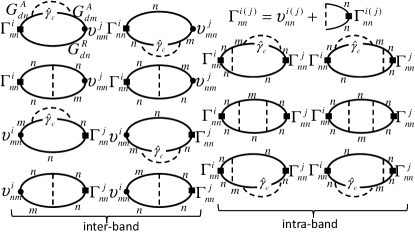
Figure 1: The SJC diagrams for $\sigma_{ij}$ expressed in the band eigenstate basis described by the indices $m$ and $n$ ($m\neq n$). The bold lines correspond to $\hat{G}_{d}^{R(A)}$ (that can be replaced by disorder-free GF’s for calculation of the SJC (Sinitsyn et al., 2007)) while dashed lines correspond to disorder strength $\mathcal{V}$. By iterating Eq. (10) and expanding as in Eq. (7), the leading-order contributions in Eq. (8) can be expressed as two components of SJC. The diagrams beginning and ending with velocity involving single (multiple) band(s) are termed as intra(inter)-band diagrams.

To obtain the remaining terms in Eq. (8) up to the zeroth order in $\mathcal{V}$ we expand Eq. (10) into an infinite series, furthermore substituting this series into Eq. (8). In the band eigenstate representation, we can further replace the GF’s via diagonal ones according to Eq. (7). The resulting infinite sum has the terms of order $\mathcal{V}^{-1}$:

$$\sigma_{ij}=\dfrac{e^{2}}{\hbar\mathcal{V}}{\displaystyle\sum_{\eta=1}^{N}}\int{\displaystyle\frac{d^{n-1}k_{\eta}}{(2\pi)^{n}}\partial_{\hbar k_{i}}\varepsilon_{\eta}\dfrac{\partial_{\hbar k_{j}}\varepsilon_{\eta}-[\hat{U}^{\dagger}\hat{P}_{j}\hat{U}]_{\eta\eta}}{2\left|\partial_{\hbar\mathbf{k}}\varepsilon_{\eta}\right|[\hat{\gamma}_{c}]_{\eta\eta}}}\;,$$

leading to the symmetric part of the conductivity, which describes the anisotropic magnetoresistance. The more interesting terms contributing to the AHE appear at zeroth order in $\mathcal{V}$ and can be graphically represented as two sets of diagrams (see Fig. 1). The inter-band diagrams, corresponding to calculating $\boldsymbol{\hat{\rho}}=\mathbf{\hat{P}}/\mathcal{V}+\mathcal{O}(\mathcal{V})$ in Eq. (8) up to the most singular (i.e., $\mathcal{V}^{-1}$) order, lead to Eq. (3). The intra-band diagrams, corresponding to calculating $\boldsymbol{\hat{\rho}}$ in Eq. (8) up to the zeroth order in $\mathcal{V}$, lead to Eq. (4). Here, $\mathbf{\hat{P}}$ is an $N\times N$ matrix given by the solution to Eq. (6), which corresponds to the leading-order vertex correction to the bare velocity captured by $\hat{\boldsymbol{\Gamma}}$.

Application to Rashba and Luttinger models.—We first apply Eqs. (2)-(4) to a Rashba ferromagnet with $\{-\Omega;\Omega\}$ band gap at $k=0$ arriving at expressions (Table I in supplementary material (supp, 2010)) consistent with the previous works (Sinitsyn et al., 2007; Kovalev et al., 2009). The vertex corrections lead to important contributions and should in general be considered.

However, for inversion-symmetric systems with $\hat{H}_{0}(\mathbf{k})=\hat{H}_{0}(-\mathbf{k})$, the vertex corrections vanish for short-ranged disorder as can be seen by inspecting the $\boldsymbol{\hat{P}}$ independent term in Eq. (6). Similar vanishing of the vertex corrections takes place in calculations of the anisotropic magnetoresistance and SHE (Murakami, 2004). We apply our theory to 4- and 6-band Luttinger (inversion-symmetric with $\boldsymbol{\hat{P}}=0$) Hamiltonians with anisotropic Luttinger parameters relevant to III-V semiconductor compounds. The spherical model Hamiltonian in the presence of splitting due to interactions with polarized Mn moments can be written as follows within the mean-field description (Abolfath et al., 2001):

$$\hat{H}_{0}=\dfrac{\hbar^{2}}{2m_{e}}\left[\left(\gamma_{1}+\dfrac{5}{2}\gamma_{2}\right)k^{2}-2\gamma_{2}(\mathbf{k}\cdot\hat{\mathbf{j}})^{2}\right]-\Omega\mathbf{m}\cdot\hat{\mathbf{s}}\;,$$ (13)

where $\hat{\mathbf{j}}$ is the angular momentum operator for $J=3/2$, $\hat{\mathbf{s}}$ is the spin operator which has to be projected onto the $J=3/2$ total angular momentum subspace ($\hat{\mathbf{s}}=\hat{\mathbf{j}}/3$) within the 4-band model, $\gamma_{1}$ and $\gamma_{2}$ are Luttinger parameters defining the light- and heavy-hole bands with the effective masses $m_{\rm lh/hh}=m_{e}/(\gamma_{1}\pm 2\gamma_{2})$, in terms of the free-electron mass $m_{e}$, $\mathbf{m}$ is the magnetization polarization direction and $\Omega$ is the mean field proportional to the average of local moments. For fully-polarized Mn spins, $\mathbf{m}$ is uniform and $\Omega=N_{\rm Mn}SJ_{\rm pd}$, where $N_{\rm Mn}$ is the density of Mn ions with spin $S=5/2$, and $J_{\rm pd}=50\leavevmode\nobreak\ {\rm meV}\,{\rm nm}^{3}$ is the strength of the exchange coupling between the local moments and the valence-band electrons (Ohno, 1999). The corresponding 6-band Hamiltonian can be found in (Abolfath et al., 2001). As the vertex corrections vanish, all terms involving $\mathbf{\hat{P}}$ in Eqs. (3) and (4) vanish, leading, up to linear order in $\Omega$, to the following analytical result for Hamiltonian (13):

$$\sigma^{\rm sj}_{yx}=\frac{\sigma_{0}}{10}\dfrac{5p(1-\sqrt{p})+3(1-p^{5/2})}{(1-p)(1+p-\sqrt{p})}\;,$$ (14)

where $\sigma_{0}=(\Omega e^{2}/3\pi^{2}\hbar^{2})\sqrt{m_{\rm hh}/2\hbar\omega_{F}}$ and $p=m_{\rm lh}/m_{\rm hh}$. SJC is in the range from $0.3\sigma_{0}$ to $\sigma_{0}$ increasing as $p\rightarrow 1$.

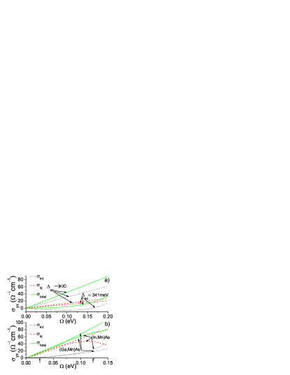
Figure 2: SJC and IC to the AHE as a function of the mean-field; (a) $\Delta_{\rm so}\rightarrow\infty$ corresponds to 4-band model and $\Delta_{\rm so}=341\leavevmode\nobreak\ {\rm meV}$ corresponds to GaAs host, the hole density is $0.35\leavevmode\nobreak\ {\rm nm}^{-3}$, (b) the plots correspond to the In/Ga,As hosts. The hole densities are $0.1\leavevmode\nobreak\ {\rm nm}^{-3}$ and $0.35\leavevmode\nobreak\ {\rm nm}^{-3}$ for the former/latter. By arrows, we mark the saturation mean-fields $\Omega=25/122\leavevmode\nobreak\ {\rm meV}$ for the In/Ga,As hosts (Ohno, 1999; Jungwirth et al., 2002).

In Fig. 2a, we present results of our calculations for the spherical 4- and 6-band Hamiltonians. The parameters are chosen to match GaAs effective masses $m_{\rm hh}=m_{e}/2$, $p=0.16$ and the SO gap $\Delta_{\rm so}=341\leavevmode\nobreak\ {\rm meV}$. The SJC does not change much as we vary $\Delta_{\rm so}$. The SJC can become dominant for the smaller SO gaps since the IC sharply diminishes eventually changing sign.

To have a more accurate description of the valence bands in III-V semiconductor compounds, one has to introduce the third phenomenological Luttinger parameter $\gamma_{3}$. This leads to band warping which has strong effect on the IC (Jungwirth et al., 2002). Our calculations show that the SJC is accelerated by the presence of band warping. In Fig. 2b, we present results of our calculations for (In/Ga,Mn)As for which $\Delta_{\rm so}=430/341\leavevmode\nobreak\ {\rm meV}$, and $(\gamma_{1},\gamma_{2},\gamma_{3})=(19.67,8.37,9.29)/(6.85,2.1,2.9)$ (Abolfath et al., 2001). In both cases, the AHE is dominated by the SJC. We use densities $N_{\rm Mn}=0.23/1.1\leavevmode\nobreak\ {\rm nm}^{-3}$ for the In/Ga,As host leading to saturation values of the effective field $\Omega=25/122\leavevmode\nobreak\ {\rm meV}$ (Ohno, 1999; Jungwirth et al., 2002). Taking the hole density as in Ref. (Jungwirth et al., 2002) ($0.1/0.35\leavevmode\nobreak\ {\rm nm}^{-3}$ for In/Ga,As host), we arrive at the AHE $\sigma_{yx}=16/85\leavevmode\nobreak\ \Omega^{-1}\,{\rm cm}^{-1}$ for (In/Ga,Mn)As. Our results for the IC agree with the previous calculations (Jungwirth et al., 2002) while the total AHE overestimates the experimental values (Ohno, 1999; Edmonds et al., 2003) which is expected as the experiments are only on the border of the metallic regime.

Summary.—We formulated a theory of the AHE for metallic noninteracting multi-band systems with the final result for the IC and SJC being expressed through the material’s electronic band structure. Our derivation relies on the minimal coupling with the electromagnetic field in Hamiltonian (1), which is justified when a sufficient number of bands is considered. (E.g., the side-jump scattering in conduction bands due to spin-orbit coupling associated with impurities (Nozieres and Lewiner, 1973) can be described within our approach by resorting to the 8-band Kane model.) In contrast to the theory of the intrinsic AHE, the electron (hole) motion in a particular band cannot be defined solely in terms of the Bloch wave functions of the same band in the presence of disorder-induced band mixing. The SJC does not depend on the disorder strength but will generally change with the type of disorder (e.g., short-range impurities vs. phonon scattering). The associated scattering regime crossovers can be accompanied by a sign change of the AHE as the IC and SJC can be of opposite sign. The AHE sign change has been observed in Fe and (Ga,Mn)As (Dheer, 1967). Ac measurements, furthermore, can quench the SJC in clean samples at intermediate frequencies $\tau^{-1}<\omega<\Delta$. We demonstrated our theory on electronic band structures of the 2D Rashba and 3D Luttinger Hamiltonians. Within our simple model, the AHE in the metallic (In/Ga,Mn)As magnetic semiconductors at low temperatures is dominated by the SJC. The proposed theory can be further used in ab initio calculations of the AHE in wide range of available metallic materials.

This work was supported in part by the DARPA, Alfred P. Sloan Foundation, NSF under Grant Nos. DMR-0840965 (YT) and DMR-0547875 (JS), and the Research Corporation for the Advancement of Science (JS).

References

Karplus and Luttinger (1954)
R. Karplus and
J. M. Luttinger,
Phys. Rev. 95,
1154 (1954).
Nagaosa et al. (2010)
N. Nagaosa,
J. Sinova,
S. Onoda,
A. H. MacDonald,
and N. P. Ong,
Rev. Mod. Phys. 82,
1539 (2010).
Sundaram and Niu (1999)
G. Sundaram and
Q. Niu,
Phys. Rev. B 59,
14915 (1999).
Mathieu et al. (2004)
R. Mathieu,
A. Asamitsu,
H. Yamada,
K. S. Takahashi,
M. Kawasaki,
Z. Fang,
N. Nagaosa, and
Y. Tokura,
Phys. Rev. Lett. 93,
016602 (2004); Y. Yao,
L. Kleinman,
A. H. MacDonald,
J. Sinova,
T. Jungwirth,
D.-s. Wang,
E. Wang, and
Q. Niu,
ibid.92,
037204 (2004); K. M. Seemann,
Y. Mokrousov,
A. Aziz,
J. Miguel,
F. Kronast,
W. Kuch,
M. G. Blamire,
A. T. Hindmarch,
B. J. Hickey,
I. Souza,
et al., ibid.104, 076402
(2010); X. Wang,
D. Vanderbilt,
J. R. Yates, and
I. Souza,
Phys. Rev. B 76,
195109 (2007).
Jungwirth et al. (2002)
T. Jungwirth,
Q. Niu, and
A. H. MacDonald,
Phys. Rev. Lett. 88,
207208 (2002); J. Sinova,
T. Jungwirth,
J. Kučera, and A. H.
MacDonald, Phys. Rev. B
67, 235203
(2003).
Tian et al. (2009)
Y. Tian,
L. Ye, and
X. Jin,
Phys. Rev. Lett. 103,
087206 (2009).
Inoue et al. (2004)
J.-I. Inoue,
G. E. Bauer,
and L. W.
Molenkamp, Phys. Rev. B
70, 041303
(2004); E. G. Mishchenko,
A. V. Shytov,
and B. I.
Halperin, Phys. Rev. Lett.
93, 226602
(2004).
Sinitsyn et al. (2007)
N. A. Sinitsyn,
A. H. MacDonald,
T. Jungwirth,
V. K. Dugaev,
and J. Sinova,
Phys. Rev. B 75,
045315 (2007); T. S. Nunner,
N. A. Sinitsyn,
M. F. Borunda,
V. K. Dugaev,
A. A. Kovalev,
A. Abanov,
C. Timm,
T. Jungwirth,
J.-I. Inoue,
A. H. MacDonald,
et al., ibid.76, 235312
(2007); A. A. Kovalev,
K. Výborný,
and J. Sinova,
ibid.78,
041305 (2008); N. A. Sinitsyn,
J. Phys.: Condens. Matter 20,
023201 (2008).
Kovalev et al. (2009)
A. A. Kovalev,
Y. Tserkovnyak,
K. Vyborny, and
J. Sinova,
Phys. Rev. B 79,
195129 (2009);
S. Onoda,
N. Sugimoto,
and
N. Nagaosa,
ibid.77,
165103 (2008).
Streda (1982)
P. Streda,
J. Phys. C 15,
L717 (1982).
supp (2010)
See supplementary material.
Murakami (2004)
S. Murakami,
Phys. Rev. B 69,
241202 (2004); M. Trushin,
K. Výborný,
P. Moraczewski,
A. A. Kovalev,
J. Schliemann,
and
T. Jungwirth,
ibid.80,
134405 (2009).
Abolfath et al. (2001)
M. Abolfath,
T. Jungwirth,
J. Brum, and
A. H. MacDonald,
Phys. Rev. B 63,
054418 (2001); T. Dietl,
H. Ohno, and
F. Matsukura,
ibid.63,
195205 (2001).
Ohno (1999)
F. Matsukura,
H. Ohno,
A. Shen, and
Y. Sugawara,
Phys. Rev. B 57,
R2037 (1998); H. Ohno,
Science 281,
951 (1998); H. Ohno,
J. Magn. Magn. Mater. 200, 110
(1999).
Edmonds et al. (2003)
K. W. Edmonds,
R. P. Campion,
K. Y. Wang,
A. C. Neumann,
B. L. Gallagher,
C. T. Foxon, and
P. C. Main,
J. Appl. Phys. 93,
6787 (2003); T. Jungwirth,
J. Sinova,
K. Y. Wang,
K. W. Edmonds,
R. P. Campion,
B. L. Gallagher,
C. T. Foxon,
Q. Niu, and
A. H. MacDonald,
Appl. Phys. Lett. 83,
320 (2003).
Dheer (1967)
P. N. Dheer,
Phys. Rev. 156,
637 (1967); D. Chiba,
A. Werpachowska,
M. Endo,
Y. Nishitani,
F. Matsukura,
T. Dietl, and
H. Ohno,
Phys. Rev. Lett. 104,
106601 (2010).
Nozieres and Lewiner (1973)
P. Nozieres and
C. Lewiner,
J. Phys. (Paris) 34,
901 (1973).