White Dwarfs in Ultrashort Binary Systems

1 Introduction

White dwarf binaries are thought to be the most common binaries in the Universe, and in our Galaxy their number is estimated to be as high as 10⁸. In addition most stars are known to be part of binary systems, roughly half of which have orbital periods short enough that the evolution of the two stars is strongly influenced by the presence of a companion. Furthermore, it has become clear from observed close binaries, that a large fraction of binaries that interacted in the past must have lost considerable amounts of angular momentum, thus forming compact binaries, with compact stellar components. The details of the evolution leading to the loss of angular momentum are uncertain, but generally this is interpreted in the framework of the so called “common-envelope evolution”: the picture that in a mass-transfer phase between a giant and a more compact companion the companion quickly ends up inside the giant’s envelope, after which frictional processes slow down the companion and the core of the giant, causing the “common envelope” to be expelled, as well as the orbital separation to shrink dramatically Taam and Sandquist (2000) .

Among the most compact binaries know, often called ultra-compact or ultra-short binaries, are those hosting two white dwarfs and classified into two types: detached binaries, in which the two components are relatively widely separated and interacting binaries, in which mass is transferred from one component to the other. In the latter class a white dwarf is accreting from a white dwarf like object (we often refer to them as AM CVn systems, after the prototype of the class, the variable star AM CVn; warn95 ; Nelemans (2005) ).

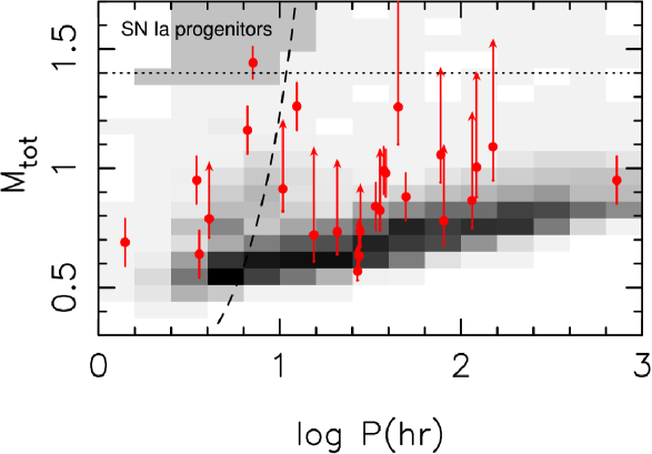
Figure 1: Period versus total mass of double white dwarfs. The points and arrows are observed systems Nelemans et al. (2005) , the grey shade a model for the Galactic population. Systems to the left of the dashed line will merge within a Hubble time, systems above the dotted line have a combined mass above the Chandrasekhar mass. The top left corner shows the region of possible type Ia supernova progenitors, where the grey shade has been darkened for better visibility (adapted from Nelemans (2007) ).

In the past many authors have emphasised the importance of studying white dwarfs in DDBs. In fact, the study of ultra-short white dwarf binaries is relevant to some important astrophysical questions which have been outlined by several author. Recently, Nelemans (2007) listed the following ones:

• Binary evolution Double white dwarfs are excellent tests of binary evolution. In particular the orbital shrinkage during the common-envelope phase can be tested using double white dwarfs. The reason is that for giants there is a direct relation between the mass of the core (which becomes a white dwarf and so its mass is still measurable today) and the radius of the giant. The latter carries information about the (minimal) separation between the two components in the binary before the common envelope, while the separation after the common envelope can be estimated from the current orbital period. This enables a detailed reconstruction of the evolution leading from a binary consisting of two main sequence stars to a close double white dwarf Nelemans et al.(2000) . The interesting conclusion of this exercise is that the standard schematic description of the common envelope – in which the envelope is expelled at the expense of the orbital energy – cannot be correct. An alternative scheme, based on the angular momentum, for the moment seems to be able to explain all the observations Nelemans and Tout (2005) .

• Type Ia supernovae Type Ia supernovae have peak brightnesses that are well correlated with the shape of their light curve Phillips (1993) , making them ideal standard candles to determine distances. The measurement of the apparent brightness of far away supernovae as a function of redshift has led to the conclusion that the expansion of the universe is accelerating Perlmutter et al. (1998) ; Riess et al.(2004) . This depends on the assumption that these far-away (and thus old) supernovae behave the same as their local cousins, which is a quite reasonable assumption. However, one of the problems is that we do not know what exactly explodes and why, so the likelihood of this assumption is difficult to assess Podsiadlowski et al. (2006) . One of the proposed models for the progenitors of type Ia supernovae are massive close double white dwarfs that will explode when the two stars merge Iben and Tutukov (1984) . In Fig. 1 the observed double white dwarfs are compared to a model for the Galactic population of double white dwarfs Nelemans et al. (2001) , in which the merger rate of massive double white dwarfs is similar to the type Ia supernova rate. The grey shade in the relevant corner of the diagram is enhanced for visibility. The discovery of at least one system in this box confirms the viability of this model (in terms of event rates).

• Accretion physics The fact that in AM CVn systems the mass losing star is an evolved, hydrogen deficient star, gives rise to a unique astrophysical laboratory, in which accretion discs made of almost pure helium Marsh et al. (1991) ; Schulz et al.(2001) ; Groot et al. (2001) ; Roelofs et al. (2006) ; Werner et al. (2006) . This opens the possibility to test the behaviour of accretion discs of different chemical composition.

• Gravitational wave emission Untill recently the DDBs with two NSs were considered among the best sources to look for gravitational wave emission, mainly due to the relatively high chirp mass expected for these sources, In fact, simply inferring the strength of the gravitational wave amplitude expected for from Evans et al. (1987)

  $$h=\left[\frac{16\pi GL_{GW}}{c^{3}\omega^{2}_{g}4\pi d^{2}}\right]^{1/2}=10^{-21}\left(\frac{{\cal{M}}}{{\it M}_{\odot}}\right)^{5/3}\left(\frac{P_{orb}}{\rm 1hr}\right)^{-2/3}\left(\frac{d}{\rm 1kpc}\right)^{-1}$$ (1)

  where

  $$L_{GW}=\frac{32}{5}\frac{G^{4}}{c^{5}}\frac{M^{2}m^{2}(m+M)}{a^{5}};$$ (2)

  $${\cal{M}}=\frac{(Mm)^{3/5}}{(M+m)^{1/5}}$$ (3)

  where the frequency of the wave is given by $f=2/P_{orb}$. It is evident that the strain signal $h$ from DDBs hosting neutron stars is a factor 5-20 higher than in the case of DDBs with white dwarfs as far as the orbital period is larger than approximatively 10-20 minutes. In recent years, AM CVns have received great attention as they represent a large population of guaranteed sources for the forthcoming Laser Interferometer Space Antenna 2006astro.ph..5722N ; 2005ApJ…633L..33S . Double WD binaries enter the LISA observational window (0.1 $\div$ 100 mHz) at an orbital period $\sim$ 5 hrs and, as they evolve secularly through GW emission, they cross the whole LISA band. They are expected to be so numerous ($\sim 10^{3}\div 10^{4}$ expected), close on average, and luminous in GWs as to create a stochastic foreground that dominates the LISA observational window up to $\approx$ 3 mHz 2005ApJ…633L..33S . Detailed knowledge of the characteristics of their background signal would thus be needed to model it and study weaker background GW signals of cosmological origin.

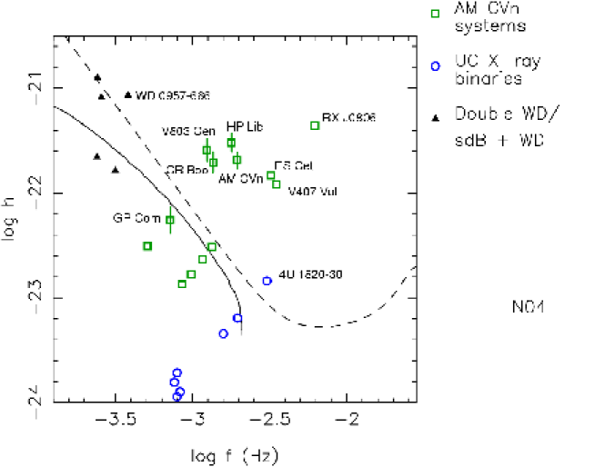
Figure 2: Expected signals of ultra-compact binaries, the ones with error bars from (adapted from Roelofs et al. (2006) ; Nelemans (2007) .

A relatively small number of ultracompact DDBs systems is presently known. According to 2006MNRAS.367L..62R there exist 17 confirmed objects with orbital periods in the $10\div 70$ min in which a hydrogen-deficient mass donor, either a semi-degenerate star or a WD itself, is present. These are called AM CVn systems and are roughly characterized by optical emission modulated at the orbital period, X-ray emission showing no evidence for a significant modulation (from which a moderately magnetic primary is suggested, 2006astro.ph.10357R ) and, in the few cases where timing analyses could be carried out, orbital spin-down consistent with GW emission-driven mass transfer.

In addition there exist two peculiar objects, sharing a number of observational properties that partially match those of the “standard” AM CVn’s. They are RX J0806.3+1527  and RX J1914.4+2456, whose X-ray emission is $\sim$ 100% pulsed, with on-phase and off-phase of approximately equal duration. The single modulations found in their lightcurves, both in the optical and in X-rays, correspond to periods of, respectively, 321.5 and 569 s (2004MSAIS…5..148I ; 2002ApJ…581..577S ) and were first interpreted as orbital periods. If so, these two objects are the binary systems with the shortest orbital period known and could belong to the AM CVn class. However, in addition to peculiar emission properties with respect to other AM CVn’s, timing analyses carried out by the above cited authors demonstrate that, in this interpretation, these two objects have shrinking orbits. This is contrary to what expected in mass transferring double white dwarf systems (including AM CVn’s systems) and suggests the possibility that the binary is detached, with the orbit shrinking because of GW emission. The electromagnetic emission would have in turn to be caused by some other kind of interaction.

Nonetheless, there are a number of alternative models to account for the observed properties, all of them based upon binary systems. The intermediate polar (IP) model (Motch et al.(1996) ; io99 ; Norton et al. (2004) ) is the only one in which the pulsation periods are not assumed to be orbital. In this model, the pulsations are likely due to the spin of a white dwarf accreting from non-degenerate secondary star. Moreover, due to geometrical constraints the orbital period is not expected to be detectable. The other two models assume a double white dwarf binaries in which the pulsation period is the orbital period. Each of them invoke a semi-detached, accreting double white dwarfs: one is magnetic, the double degenerate polar model (crop98 ; ram02a ; ram02b ; io02a ), while the other is non-magnetic, the direct impact model (Nelemans et al. (2001) ; Marsh and Steeghs(2002) ; ram02a ), in which, due to the compact dimensions of these systems, the mass transfer streams is forced to hit directly onto the accreting white dwarfs rather than to form an accretion disk .

Table 1: Overview of observational properties of AM CVn stars (adapted from Nelemans (2005) )

Name	$P_{\rm orb}^{a}$		$P_{\rm sh}^{a}$	Spectrum	Phot. varb	dist	X-rayc	UVd
	(s)		(s)			(pc)
ES Cet	621	(p/s)		Em	orb	350	C3X	GI
AM CVn	1029	(s/p)	1051	Abs	orb	606${}^{+135}_{-95}$	RX	HI
HP Lib	1103	(p)	1119	Abs	orb	197${}^{+13}_{-12}$	X	HI
CR Boo	1471	(p)	1487	Abs/Em?	OB/orb	337${}^{+43}_{-35}$	ARX	I
KL Dra	1500	(p)	1530	Abs/Em?	OB/orb
V803 Cen	1612	(p)	1618	Abs/Em?	OB/orb		Rx	FHI
SDSSJ0926+36	1698.6	(p)			orb
CP Eri	1701	(p)	1716	Abs/Em	OB/orb			H
2003aw	?		2042	Em/Abs?	OB/orb
SDSSJ1240-01	2242	(s)		Em	n
GP Com	2794	(s)		Em	n	75$\pm 2$	ARX	HI
CE315	3906	(s)		Em	n	77?	R(?)X	H
Candidates
RXJ0806+15	321	(X/p)		He/H?11	“orb”		CRX
V407 Vul	569	(X/p)		K-star16	“orb”		ARCRxX

$a$ orb = orbital, sh = superhump, periods from ww03, see references therein, (p)/(s)/(X) for photometric, spectroscopic, X-ray period.
$b$ orb = orbital, OB = outburst
$c$ A = ASCA, C = Chandra, R = ROSAT, Rx = RXTE, X = XMM-Newton kns+04
$d$ F = FUSE, G = GALEX, H = HST, I = IUE

After a brief presentation of the two X–ray selected double degenerate binary systems, we discuss the main scenario of this type, the Unipolar Inductor Model (UIM) introduced by 2002MNRAS.331..221W and further developed by 2006A&A…447..785D ; 2006astro.ph..3795D , and compare its predictions with the salient observed properties of these two sources.

1.1 RX J0806.3+1527

RX J0806.3+1527 was discovered in 1990 with the ROSAT satellite during the All-Sky Survey (RASS; beu99 ). However, it was only in 1999 that a periodic signal at 321 s was detected in its soft X-ray flux with the ROSAT HRI (io99 ; bur01 ). Subsequent deeper optical studies allowed to unambiguously identify the optical counterpart of RX J0806.3+1527, a blue $V=21.1$ ($B=20.7$) star (io02a ; io02b ). $B$, $V$ and $R$ time-resolved photometry revealed the presence of a $\sim 15$% modulation at the $\sim 321$ s X-ray period (io02b ; ram02a .

Figure 3: VLT FORS1 medium (6Å; 3900–6000Å) and low (30Å; above 6000Å) resolution spectra obtained for the optical counterpart of RX J0806.3+1527. Numerous faint emission lines of HeI and HeII (blended with H) are labeled (adapted form io02b ).

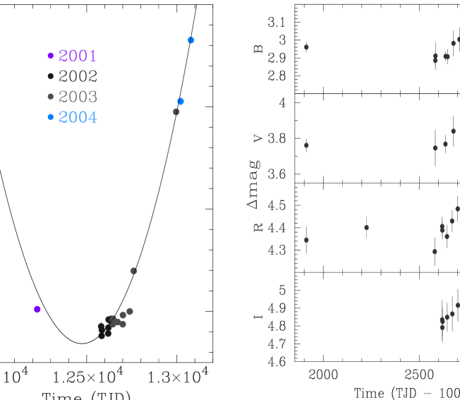
Figure 4: Left panel: Results of the phase fitting technique used to infer the P-Ṗ coherent solution for RX J0806.3+1527: the linear term (P component) has been corrected, while the quadratic term (the Ṗ component) has been kept for clarity. The best Ṗ solution inferred for the optical band is marked by the solid fit line. Right panel: 2001-2004 optical flux measurements at fdifferent wavelengths.

The VLT spectral study revealed a blue continuum with no intrinsic absorption lines io02b . Broad ($\rm FWHM\sim 1500~{}\rm km~{}s^{-1}$), low equivalent width ($EW\sim-2\div-6$ Å) emission lines from the He II Pickering series (plus additional emission lines likely associated with He I, C III, N III, etc.; for a different interpretation see rei04 ) were instead detected io02b . These findings, together with the period stability and absence of any additional modulation in the 1 min–5 hr period range, were interpreted in terms of a double degenerate He-rich binary (a subset of the AM CVn class; see warn95 ) with an orbital period of 321 s, the shortest ever recorded. Moreover, RX J0806.3+1527 was noticed to have optical/X-ray properties similar to those of RX J1914.4+2456, a 569 s modulated soft X-ray source proposed as a double degenerate system (crop98 ; ram00 ; ram02b ).

In the past years the detection of spin–up was reported, at a rate of $\sim$6.2$\times$10^-11  s s^-1, for the 321 s orbital modulation, based on optical data taken from the Nordic Optical Telescope (NOT) and the VLT archive, and by using incoherent timing techniques hak03 ; hak04 . Similar results were reported also for the X-ray data (ROSAT and Chandra; stro03 ) of RX J0806.3+1527 spanning over 10 years of uncoherent observations and based on the NOT results hak03 .

A Telescopio Nazionale Galileo (TNG) long-term project (started on 2000) devoted to the study of the long-term timing properties of RX J0806.3+1527  found a slightly energy–dependent pulse shape with the pulsed fraction increasing toward longer wavelengths, from $\sim$12% in the B-band to nearly 14% in the I-band (see lower right panel of Figure 5; 2004MSAIS…5..148I ). An additional variability, at a level of 4% of the optical pulse shape as a function of time (see upper right panel of Figure 5 right) was detected. The first coherent timing solution was also inferred for this source, firmly assessing that the source was spinning-up: P=321.53033(2) s, and Ṗ=-3.67(1)$\times$10^-11 s s^-1 (90% uncertainties are reported; 2004MSAIS…5..148I ). Reference 2005ApJ…627..920S obtained independently a phase-coherent timing solutions for the orbital period of this source over a similar baseline, that is fully consistent with that of 2004MSAIS…5..148I . See 2007MNRAS.374.1334B for a similar coherent timing solution also including the covariance terms of the fitted parameters.

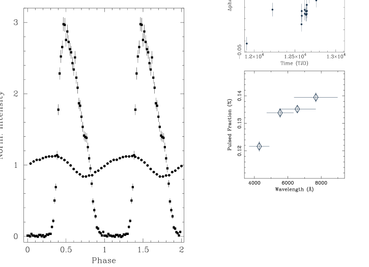
Figure 5: Left Panel: The 1994–2002 phase coherently connected X–ray folded light curves (filled squares; 100% pulsed fraction) of RX J0806.3+1527, together with the VLT-TNG 2001-2004 phase connected folded optical light curves (filled circles). Two orbital cycles are reported for clarity. A nearly anti-correlation was found. Right panels: Analysis of the phase variations induced by pulse shape changes in the optical band (upper panel), and the pulsed fraction as a function of optical wavelengths (lower panel).

The relatively high accuracy obtained for the optical phase coherent P-Ṗ solution (in the January 2001 - May 2004 interval) was used to extend its validity backward to the ROSAT observations without loosing the phase coherency, i.e. only one possible period cycle consistent with our P-Ṗ solution. The best X–ray phase coherent solution is P=321.53038(2) s, Ṗ=-3.661(5)$\times$10^-11 s s^-1 (for more details see 2004MSAIS…5..148I ). Figure 5 (left panel) shows the optical (2001-2004) and X–ray (1994-2002) light curves folded by using the above reported P-Ṗ coherent solution, confirming the amazing stability of the X–ray/optical anti-correlation first noted by (2003ApJ…598..492I ; see inset of left panel of Figure 5).

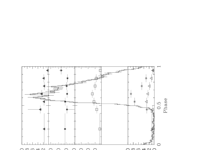
Figure 6: The results of the XMM–Newton phase-resolved spectroscopy (PRS) analysis for the absorbed blackbody spectral parameters: absorption, blackbody temperature, blackbody radius (assuming a distance of 500 pc), and absorbed (triangles) and unabsorbed (asterisks) flux. Superposed is the folded X-ray light curve.

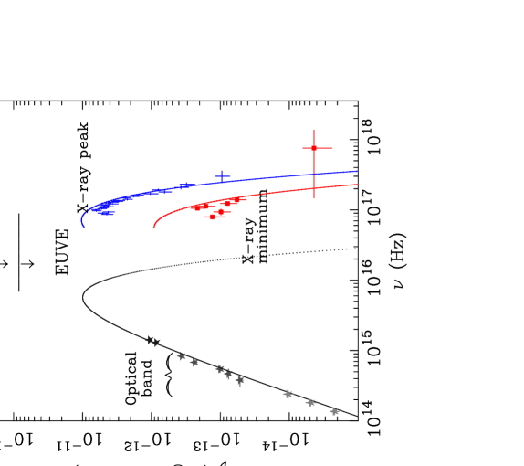
Figure 7: Broad-band energy spectrum of RX J0806.3+1527 as inferred from the Chandra, XMM–Newton, VLT and TNG measurements and EUVE upper limits. The dotted line represents one of the possible fitting blackbody models for the IR/optical/UV bands.

On 2001, a Chandra observation of RX J0806.3+1527 carried out in simultaneity with time resolved optical observation at the VLT, allowed for the first time to study the details of the X-ray emission and the phase-shift between X-rays and optical band. The X-ray spectrum is consistent with a occulting, as a function of modulation phase, black body with a temperature of $\sim$60 eV 2003ApJ…598..492I . A 0.5 phase-shift was reported for the X-rays and the optical band 2003ApJ…598..492I . More recently, a 0.2 phase-shift was reported by analysing the whole historical X-ray and optical dataset: this latter result is considered the correct one 2007MNRAS.374.1334B .

On 2002 November 1^st a second deep X-ray observation was obtained with the XMM–Newton instrumentations for about 26000 s, providing an increased spectral accuracy (see eft panel of Figure 7). The XMM–Newton data show a lower value of the absorption column, a relatively constant black body temperature, a smaller black body size, and, correspondingly, a slightly lower flux. All these differences may be ascribed to the pile–up effect in the Chandra data, even though we can not completely rule out the presence of real spectral variations as a function of time. In any case we note that this result is in agreement with the idea of a self-eclipsing (due only to a geometrical effect) small, hot and X–ray emitting region on the primary star. Timing analysis did not show any additional significant signal at periods longer or shorter than 321.5 s, (in the 5hr-200ms interval). By using the XMM–Newton OM a first look at the source in the UV band (see right panel of Figure 7) was obtained confirming the presence of the blackbody component inferred from IR/optical bands.

Reference 2003ApJ…598..492I measured an on-phase X-ray luminosity (in the range 0.1-2.5 keV) $L_{X}=8\times 10^{31}(d/200~{}\mbox{pc})^{2}$ erg s^-1 for this source. These authors suggested that the bolometric luminosity might even be dominated by the (unseen) value of the UV flux, and reach values up to 5-6 times higher. The optical flux is only $\sim$ 15% pulsed, indicating that most of it might not be associated to the same mechanism producing the pulsed X-ray emission (possibly the cooling luminosity of the WD plays a role). Given these uncertainties and, mainly, the uncertainty in the distance to the source, a luminosity $W\simeq 10^{32}(d/200~{}\mbox{pc})^{2}$ erg s^-1 will be assumed as a reference value.

1.2 RX J1914.4+2456 

The luminosity and distance of this source have been subject to much debate over the last years. Reference 2002MNRAS.331..221W refer to earlier ASCA measurements that, for a distance of 200-500 pc, corresponded to a luminosity in the range ($4\times 10^{33}\div 2.5\times 10^{34}$) erg s^-1. Reference 2005MNRAS.357…49R , based on more recent XMM-Newton observations and a standard blackbody fit to the X-ray spectrum, derived an X-ray luminosity of $\simeq 10^{35}d^{2}_{\mbox{\tiny{kpc}}}$ erg s^-1, where $d_{\mbox{\tiny{kpc}}}$ is the distance in kpc. The larger distance of $\sim$ 1 kpc was based on a work by 2006ApJ…649..382S . Still more recently, 2006MNRAS.367L..62R find that an optically thin thermal emission spectrum, with an edge at 0.83 keV attributed to O VIII, gives a significantly better fit to the data than a blackbody model. The optically thin thermal plasma model implies a much lower bolometric luminosity of L${}_{\mbox{\tiny{bol}}}\simeq 10^{33}$ d${}^{2}_{\mbox{\tiny{kpc}}}$ erg s^-1.
Reference 2006MNRAS.367L..62R also note that the determination of a 1 kpc distance is not free of uncertainties and that a minimum distance of $\sim 200$ pc might still be possible: the latter leads to a minimum luminosity of $\sim 3\times 10^{31}$ erg s^-1.
Given these large discrepancies, interpretation of this source’s properties remains ambiguous and dependent on assumptions. In the following, we refer to the more recent assessment by 2006MNRAS.367L..62R of a luminosity $L=10^{33}$ erg s^-1 for a 1 kpc distance.
Reference 2006MNRAS.367L..62R also find possible evidence, at least in a few observations, of two secondary peaks in power spectra. These are very close to ($\Delta\nu\simeq 5\times 10^{-5}$ Hz) and symmetrically distributed around the strongest peak at $\sim 1.76\times 10^{-3}$ Hz. References 2006MNRAS.367L..62R and 2006ApJ…649L..99D discuss the implications of this possible finding.

2 The Unipolar Inductor Model

The Unipolar Inductor Model (UIM) was originally proposed to explain the origin of bursts of decametric radiation received from Jupiter, whose properties appear to be strongly influenced by the orbital location of Jupiter’s satellite Io 1969ApJ…156…59G ; 1977Moon…17..373P .
The model relies on Jupiter’s spin being different from the system orbital period (Io spin is tidally locked to the orbit). Jupiter has a surface magnetic field $\sim$ 10 G so that, given Io’s good electrical conductivity ($\sigma$), the satellite experiences an e.m.f. as it moves across the planet’s field lines along the orbit. The e.m.f. accelerates free charges in the ambient medium, giving rise to a flow of current along the sides of the flux tube connecting the bodies. Flowing charges are accelerated to mildly relativistic energies and emit coherent cyclotron radiation through a loss cone instability (cfr. Willes and Wu(2004) and references therein): this is the basic framework in which Jupiter decametric radiation and its modulation by Io’s position are explained. Among the several confirmations of the UIM in this system, HST UV observations revealed the localized emission on Jupiter’s surface due to flowing particles hitting the planet’s surface - the so-called Io’s footprint Clarke et al. (1996) . In recent years, the complex interaction between Io-related free charges (forming the Io torus) and Jupiter’s magnetosphere has been understood in much greater detail Russ1998P&SS…47..133R ; Russ2004AdSpR..34.2242R . Despite these significant complications, the above scenario maintains its general validity, particularly in view of astrophysical applications.
Reference 2002MNRAS.331..221W considered the UIM in the case of close white dwarf binaries. They assumed a moderately magnetized primary, whose spin is not synchronous with the orbit and a non-magnetic companion, whose spin is tidally locked. They particularly highlight the role of ohmic dissipation of currents flowing through the two WDs and show that this occurs essentially in the primary atmosphere. A small bundle of field lines leaving the primary surface thread the whole secondary. The orbital position of the latter is thus “mapped” to a small region onto the primary’s surface; it is in this small region that ohmic dissipation - and the associated heating - mainly takes place. The resulting geometry, illustrated in Fig. 8, naturally leads to mainly thermal, strongly pulsed X-ray emission, as the secondary moves along the orbit.

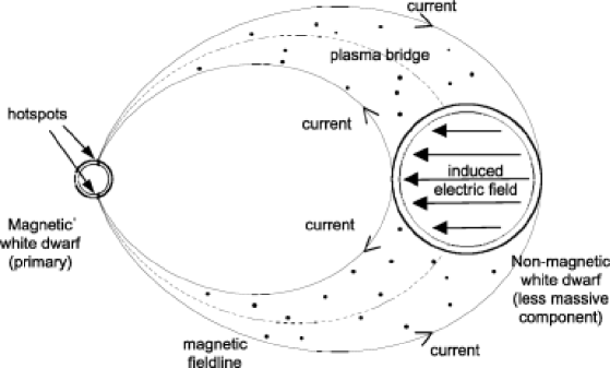
Figure 8: Electric coupling between the asynchronous, magnetic primary star and the non-magnetic secondary,, in the UIM (adapted from 2002MNRAS.331..221W ).

The source of the X-ray emission is ultimately represented by the relative motion between primary spin and orbit, that powers the electric circuit. Because of resistive dissipation of currents, the relative motion is eventually expected to be cancelled. This in turn requires angular momentum to be redistributed between spin and orbit in order to synchronize them. The necessary torque is provided by the Lorentz force on cross-field currents within the two stars.
Reference 2002MNRAS.331..221W derived synchronization timescales $(\tau_{\alpha})\sim$ few 10³ yrs for both RX J1914.4+2456  and RX J0806.3+1527 , less than 1% of their orbital evolutionary timescales. This would imply a much larger Galactic population of such systems than predicted by population-synthesis models, a major difficulty of this version of the UIM. However, 2006A&A…447..785D ; 2006astro.ph..3795D have shown that the electrically active phase is actually long-lived because perfect synchronism is never reached. In a perfectly synchronous system the electric circuit would be turned off, while GWs would still cause orbital spin-up. Orbital motion and primary spin would thus go out of synchronism, which in turn would switch the circuit on. The synchronizing (magnetic coupling) and de-synchronizing (GWs) torques are thus expected to reach an equilibrium state at a sufficiently small degree of asynchronism.
We discuss in detail how the model works and how the major observed properties of RX J0806.3+1527  and RX J1914.4+2456  can be interpreted in the UIM framework. We refer to 2005MNRAS.357.1306B for a possible criticism of the model based on the shape of the pulsed profiles of the two sources. Finally, we refer to 2006ApJ…653.1429D ; 2006ApJ…649L..99D , who have recently proposed alternative mass transfer models that can also account for long-lasting episodes of spin-up in Double White Dwarf systems.

3 UIM in Double Degenerate Binaries

According to 2002MNRAS.331..221W , define the primary’s asynchronism parameter $\alpha\equiv\omega_{1}/\omega_{o}$, where $\omega_{1}$ and $\omega_{o}$ are the primary’s spin and orbital frequencies. In a system with orbital separation $a$, the secondary star will move with the velocity $v=a(\omega_{o}-\omega_{1})=[GM_{1}(1+q)]^{1/3}~{}\omega^{1/3}_{o}(1-\alpha)$ relative to field lines, where $G$ is the gravitational constant, $M_{1}$ the primary mass, $q=M_{2}/M_{1}$ the system mass-ratio. The electric field induced through the secondary is thus $E$ = $\frac{\mbox{{\boldmath$v\times B_{2}$}}}{c}$, with an associated e.m.f. $\Phi=2R_{2}E$, $R_{2}$ being the secondary’s radius and $B$₂ the primary magnetic field at the secondary’s location. The internal (Lorentz) torque redistributes angular momentum between spin and orbit conserving their sum (see below), while GW-emission causes a net loss of orbital angular momentum. Therefore, as long as the primary spin is not efficiently affected by other forces, i.e. tidal forces (cfr. App.A in 2006A&A…447..785D ), it will lag behind the evolving orbital frequency, thus keeping electric coupling continuously active.
Since most of the power dissipation occurs at the primary atmosphere (cfr. 2002MNRAS.331..221W ), we slightly simplify our treatment assuming no dissipation at all at the secondary. In this case, the binary system is wholly analogous to the elementary circuit of Fig. 9.

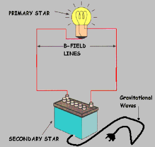
Figure 9: Sketch of the elementary circuit envisaged in the UIM. The secondary star acts as the battery, the primary star represents a resistance connected to the battery by conducting “wires” (field lines.) Inclusion of the effect of GWs corresponds to connecting the battery to a plug, so that it is recharged at some given rate. Once the battery initial energy reservoir is consumed, the bulb will be powered just by the energy fed through the plug. This corresponds to the “steady-state” solution.

Given the e.m.f. ($\Phi$) across the secondary star and the system’s effective resistivity ${\cal{R}}\approx(2\sigma R_{2})^{-1}~{}(a/R_{1})^{3/2}$, the dissipation rate of electric current ($W$) in the primary atmosphere is:

$$W=I^{2}{\cal{R}}=I\Phi=k\omega^{17/3}_{o}(1-\alpha)^{2}$$ (4)

where $k=2(\mu_{1}/c)^{2}\sigma R^{3/2}_{1}R^{3}_{2}/[GM_{1}(1+q)]^{11/6}$ is a constant of the system.
The Lorentz torque ($N_{L}$) has the following properties: i) it acts with the same magnitude and opposite signs on the primary star and the orbit, $N_{L}=N^{(1)}_{L}=-N^{(\mbox{\tiny{orb}})}_{L}$. Therefore; ii) $N_{L}$ conserves the total angular momentum in the system, transferring all that is extracted from one component to the other one; iii) $N_{L}$ is simply related to the energy dissipation rate: $W=N_{L}\omega_{o}(1-\alpha)$.
From the above, the evolution equation for $\omega_{1}$ is:

$$\dot{\omega}_{1}=(N_{L}/I_{1})=\frac{W}{I_{1}\omega_{o}(1-\alpha)}$$ (5)

The orbital angular momentum is $L_{o}=I_{o}\omega_{o}$, so that the orbital evolution equation is:

$$\dot{\omega}_{o}=-3(N_{\mbox{\tiny{gw}}}+N^{(\mbox{\tiny{orb}})}_{L})/I_{o}=-3(N_{\mbox{\tiny{gw}}}-N_{L})/I_{o}=-\frac{3}{I_{o}\omega_{o}}\left(\dot{E}_{\mbox{\tiny{gw}}}-\frac{W}{1-\alpha}\right)$$ (6)

where $I_{o}=q(1+q)^{-1/3}G^{2/3}M^{5/3}_{1}\omega^{-4/3}_{o}$ is the orbital moment of inertia and $N_{\mbox{\tiny{gw}}}=\dot{E}_{\mbox{\tiny{gw}}}/\omega_{o}$ is the GW torque.

3.1 Energetics of the electric circuit

Let us focus on how energy is transferred and consumed by the electric circuit. We begin considering the rate of work done by $N_{L}$ on the orbit

$$\dot{E}^{(orb)}_{L}=N^{(orb)}_{L}\omega_{o}=-N_{L}\omega_{o}=-\frac{W}{1-\alpha},$$ (7)

and that done on the primary:

$$\dot{E}_{spin}=N_{L}\omega_{1}=\frac{\alpha}{1-\alpha}W=-\alpha\dot{E}^{(orb)}_{L}.$$ (8)

The sum $\dot{E}_{spin}+\dot{E}^{(orb)}_{L}=-W$. Clearly, not all of the energy extracted from one component is transferred to the other one. The energy lost to ohmic dissipation represents the energetic cost of spin-orbit coupling.
The above formulae allow to draw some further conclusions concerning the relation between $\alpha$ and the energetics of the electrical circuit. When $\alpha>1$, the circuit is powered at the expenses of the primary’s spin energy. A fraction $\alpha^{-1}$ of this energy is transferred to the orbit, the rest being lost to ohmic dissipation. When $\alpha<1$, the circuit is powered at the expenses of the orbital energy and a fraction $\alpha$ of this energy is transferred to the primary spin. Therefore, the parameter $\alpha$ represents a measure of the energy transfer efficiency of spin-orbit coupling: the more asynchronous a system is, the less efficiently energy is transferred, most of it being dissipated as heat.

3.2 Stationary state: General solution

As long as the asynchronism parameter is sufficiently far from unity, its evolution will be essentially determined by the strength of the synchronizing (Lorentz) torque, the GW torque being of minor relevance. The evolution in this case depends on the initial values of $\alpha$ and $\omega_{o}$, and on stellar parameters. This evolutionary phase drives $\alpha$ towards unity, i.e. spin and orbit are driven towards synchronism. It is in this regime that the GW torque becomes important in determining the subsequent evolution of the system.
Once the condition $\alpha=1$ is reached, indeed, GW emission drives a small angular momentum disequilibrium. The Lorentz torque is in turn switched on to transfer to the primary spin the amount of angular momentum required for it to keep up with the evolving orbital frequency. This translates to the requirement that $\dot{\omega}_{1}=\dot{\omega}_{o}$. By use of expressions (5) and (6), it is found that this condition implies the following equilibrium value for $\alpha$ (we call it $\alpha_{\infty})$:

$$1-\alpha_{\infty}=\frac{I_{1}}{k}\frac{\dot{\omega}_{o}/\omega_{o}}{\omega^{11/3}}$$ (9)

This is greater than zero if the orbit is shrinking ($\dot{\omega}_{o}>0$), which implies that $\alpha_{\infty}<1$. For a widening orbit, on the other hand, $\alpha_{\infty}>1$. However, this latter case does not correspond to a long-lived configuration. Indeed, define the electric energy reservoir as $E_{UIM}\equiv(1/2)I_{1}(\omega^{2}_{1}-\omega^{2}_{o})$, which is negative when $\alpha<1$ and positive when $\alpha>1$. Substituting eq. (9) into this definition:

$$\dot{E}_{UIM}=-W,$$ (10)

If $\alpha=\alpha_{\infty}>1$, energy is consumed at the rate W: the circuit will eventually switch off ($\alpha_{\infty}=1$). At later times, the case $\alpha_{\infty}<1$ applies.
If $\alpha=\alpha_{\infty}<1$, condition (10) means that the battery recharges at the rate $W$ at which electric currents dissipate energy: the electric energy reservoir is conserved as the binary evolves.
The latter conclusion can be reversed (cfr. Fig. 9): in steady-state, the rate of energy dissipation ($W$) is fixed by the rate at which power is fed to the circuit by the plug ($\dot{E}_{UIM}$). The latter is determined by GW emission and the Lorentz torque and, therefore, by component masses, $\omega_{o}$ and $\mu_{1}$.
Therefore the steady-state degree of asynchronism of a given binary system is uniquely determined, given $\omega_{o}$. Since both $\omega_{o}$ and $\dot{\omega}_{o}$ evolve secularly, the equilibrium state will be “quasi-steady”, $\alpha_{\infty}$ evolving secularly as well.

3.3 Model application: equations of practical use

We have discussed in previous sections the existence of an asymptotic regime in the evolution of binaries in the UIM framework. Given the definition of $\alpha_{\infty}$ and $W$ (eq. 9 and 4, respectively), we have:

$$W=I_{1}\omega_{o}\dot{\omega}_{o}~{}\frac{(1-\alpha)^{2}}{1-\alpha_{\infty}}.$$ (11)

The quantity $(1-\alpha_{\infty})$ represents the actual degree of asynchronism only for those systems that had enough time to evolve towards steady-state, i.e with sufficiently short orbital period. In this case, the steady-state source luminosity can thus be written as:

$$W_{\infty}=I_{1}\dot{\omega}_{o}\omega_{o}(1-\alpha_{\infty})$$ (12)

Therefore - under the assumption that a source is in steady-state - the quantity $\alpha_{\infty}$ can be determined from the measured values of $W$, $\omega_{o}$, $\dot{\omega}_{o}$. Given its definition (eq. 9), this gives an estimate of $k$ and, thus, $\mu_{1}$.
The equation for the orbital evolution (6) provides a further relation between the three measured quantities, component masses and degree of asynchronism. This can be written as:

$$\dot{E}_{\mbox{\tiny{gr}}}+\frac{1}{3}I_{o}\omega^{2}_{o}(\dot{\omega}_{o}/\omega_{o})=\frac{W}{(1-\alpha)}$$

that becomes, inserting the appropriate expressions for $\dot{E}_{\mbox{\tiny{gr}}}$ and $I_{o}$:

$$\frac{32}{5}\frac{G^{7/3}}{c^{5}}~{}\omega^{10/3}_{o}X^{2}-\frac{1}{3}~{}G^{2/3}\frac{\dot{\omega}_{o}}{\omega^{1/3}_{o}}X+\frac{W}{1-\alpha}=0~{},$$ (13)

where $X\equiv M^{5/3}_{1}q/(1+q)^{1/3}={\cal{M}}^{5/3}$, $\cal{M}$ being the system’s chirp mass.

4 RX J0806.3+1527 

We assume here the values of $\omega_{o}$, $\dot{\omega}_{o}$ and of the bolometric luminosity reported in 1 and refer to See 2006astro.ph..3795D for a complete discussion on how our conclusions depend on these assumptions.
In Fig. 10 (see caption for further details), the dashed line represents the locus of points in the $M_{2}$ vs. $M_{1}$ plane, for which the measured $\omega_{o}$ and $\dot{\omega}_{o}$ are consistent with being due to GW emission only, i.e. if spin-orbit coupling was absent ($\alpha=1$). This corresponds to a chirp mass ${\cal{M}}\simeq$ 0.3 M_⊙.
Inserting the measured quantities in eq. (11) and assuming a reference value of $I_{1}=3\times 10^{50}$ g cm², we obtain:

$$\frac{(1-\alpha)^{2}}{1-\alpha_{\infty}}\simeq\frac{10^{32}d^{2}_{200}}{1.3\times 10^{34}}\simeq 8\times 10^{-3}d^{2}_{200}.$$ (14)

In principle, the source may be in any regime, but our aim is to check whether it can be in steady-state, as to avoid the short timescale problem mentioned in 2. Indeed, the short orbital period strongly suggests it may have reached the asymptotic regime (cfr. 2006astro.ph..3795D ). If we assume $\alpha=\alpha_{\infty}$, eq. (14) implies $(1-\alpha_{\infty})\simeq 8\times 10^{-3}$.
Once UIM and spin-orbit coupling are introduced, the locus of allowed points in the M₂ vs. M₁ plane is somewhat sensitive to the exact value of $\alpha$: the solid curve of Fig. 10 was obtained, from eq. (13), for $\alpha=\alpha_{\infty}=0.992$.
From this we conclude that, if RX J0806.3+1527  is interpreted as being in the UIM steady-state, $M_{1}$ must be smaller than 1.1 $M_{\odot}$ in order for the secondary not to fill its Roche lobe, thus avoiding mass transfer.

Figure 10: M₂ vs. M₁ plot based on the measured timing properties of RX J0806.3+1527 . The dashed curve is the locus expected if orbital decay is driven by GW alone, with no spin-orbit coupling. The solid line describes the locus expected if the system is in a steady-state, with $(1-\alpha)=(1-\alpha_{\infty})\simeq 8\times 10^{-3}$. The horizontal dot-dashed line represents the minimum mass for a degenerate secondary not to fill its Roche-lobe at an orbital period of 321.5 s. Dotted lines are the loci of fixed mass ratio.

From $(1-\alpha_{\infty})=8\times 10^{-3}$ and from eq. (4), $k\simeq 7.7\times 10^{45}$ (c.g.s.): from this, component masses and primary magnetic moment can be constrained. Indeed, $k=\hat{k}(\mu_{1},M_{1},q;\overline{\sigma})$ (eq. 4) and a further constraint derives from the fact that $M_{1}$ and $q$ must lie along the solid curve of Fig. 10. Given the value of $\overline{\sigma}$, $\mu_{1}$ is obtained for each point along the solid curve. We assume an electrical conductivity of $\overline{\sigma}=3\times 10^{13}$ e.s.u. 2002MNRAS.331..221W ; 2006astro.ph..3795D .
The values of $\mu_{1}$ obtained in this way, and the corresponding field at the primary’s surface, are plotted in Fig. 11, from which $\mu_{1}\sim$ a few $\times 10^{30}$ G cm³ results, somewhat sensitive to the primary mass.
We note further that, along the solid curve of Fig. 10, the chirp mass is slightly variable, being: $X\simeq(3.4\div 4.5)\times 10^{54}$ g^5/3, which implies ${\cal{M}}\simeq(0.26\div 0.31)$ M_⊙. More importantly, $\dot{E}_{\mbox{\tiny{gr}}}\simeq(1.1\div 1.9)\times 10^{35}$ erg s^-1 and, since $W/(1-\alpha_{\infty})=\dot{E}^{(orb)}_{L}\simeq 1.25\times 10^{34}$ erg s^-1, we have $\dot{E}_{\mbox{\tiny{gr}}}\simeq(9\div 15)~{}\dot{E}^{(orb)}_{L}$. Orbital spin-up is essentially driven by GW alone; indeed, the dashed and solid curves are very close in the M₂ vs. M₁ plane.

Figure 11: The value of the primary magnetic moment $\mu_{1}$, and the corresponding surface B-field, as a function of the primary mass M₁, for $(1-\alpha)=(1-\alpha_{\infty})=8\times 10^{-3}$.

Summarizing, the observational properties of RX J0806.3+1527  can be well interpreted in the UIM framework, assuming it is in steady-state. This requires the primary to have $\mu_{1}\sim 10^{30}$ G cm³ and a spin just slightly slower than the orbital motion (the difference being less than $\sim 1$%).
The expected value of $\mu_{1}$ can in principle be tested by future observations, through studies of polarized emission at optical and/or radio wavelenghts Willes and Wu(2004) .

5 RX J1914.4+2456 

As for the case of RX J0806.3+1527 , we adopt the values discussed in 1 and refer to 2006astro.ph..3795D for a discussion of all the uncertainties on these values and their implications for the model.
Application of the scheme used for RX J0806.3+1527  to this source is not as straightforward. The inferred luminosity of this source seems inconsistent with steady-state. With the measured values of $\omega_{o}$ and $\dot{\omega}_{o}$, the system steady-state luminosity should be $<2\times 10^{32}$ erg s^-1 (eq. 12). This is hardly consistent even with the smallest possible luminosity referred to in 1, unless allowing for a large value of ($1-\alpha_{\infty}\geq 0.15$).
From eq. (11) a relatively high ratio between the actual asynchronism parameter and its steady-state value appears unavoidable:

$$|1-\alpha|\simeq 2.2(1-\alpha_{\infty})^{1/2}$$ (15)

The case for $\alpha>1$

The low rate of orbital shrinking measured for this source and its relatively high X-ray luminosity put interesting constraints on the primary spin. Indeed, a high value of $N_{L}$ is associated to $W\sim 10^{33}$ erg s^-1.
If $\alpha<1$, this torque sums to the GW torque: the resulting orbital evolution would thus be faster than if driven by GW alone. In fact, for $\alpha<1$, the smallest possible value of $N_{L}$ obtains with $\alpha=0$, from which $N^{(\mbox{\tiny{min}})}_{L}=9\times 10^{34}$ erg. This implies an absolute minimum to the rate of orbital shrinking (eq. 6), $3~{}N^{(\mbox{\tiny{min}})}_{L}/I_{o}$, so close to the measured one that unplausibly small component masses would be required for $\dot{E}_{\mbox{\tiny{gr}}}$ to be negligible. We conclude that $\alpha<1$ is essentially ruled out in the UIM discussed here.
If $\alpha>1$ the primary spin is faster than the orbital motion and the situation is different. Spin-orbit coupling has an opposite sign with respect to the GW torque. The small torque on the orbit implied by the measured $\dot{\omega}_{o}$ could result from two larger torques of opposite signs partially cancelling each other.
This point has been overlooked by Marsh and Nelemans (2005) who estimated the GW luminosity of the source from its measured timing parameters and, based on this estimate, claimed the failure of the UIM for RX J1914.4+2456 . In discussing this and other misinterpretations of the UIM in the literature, 2006astro.ph..3795D show that the argument by Marsh and Nelemans (2005) actually leads to our same conclusion: in the UIM framework, the orbital evolution of this source must be affected significantly by spin-orbit coupling, being slowed down by the transfer of angular momentum and energy from the primary spin to the orbit. The source GW luminosity must accordingly be larger than indicated by its timing parameters.

5.1 Constraining the asynchronous system

Given that the source is not compatible with steady-state, we constrain system parameters in order to match the measured values of $W,\omega_{o}$ and $\dot{\omega}_{o}$ and meet the requirement that the resulting state has a sufficiently long lifetime.

Figure 12: M₂ vs. M₁ plot based on measured timing properties of RX J1914.4+2456 . The dot-dashed line corresponds to the minimum mass for a degenerate secondary not to fill its Roche-lobe. The dashed curve represents the locus expected if orbital decay was driven by GW alone, with no spin-orbit coupling. This curve is consistent with a detached system only for extremely low masses. The solid lines describe the loci expected if spin-orbit coupling is present (the secondary spin being always tidally locked) and gives a negative contribution to $\dot{\omega}_{o}$. The four curves are obtained for $W=10^{33}$ erg s^-1 and four different values of $\alpha=1.025,1.05,1.075$, $1.1$, respectively, from top to bottom, as reported in the plot.

Since system parameters cannot all be determined uniquely, we adopt the following scheme: given a value of $\alpha$ eq. (13) allows to determine, for each value of M₁, the corresponding value of M₂ (or $q$) that is compatible with the measured $W,\omega_{o}$ and $\dot{\omega}_{o}$. This yields the solid curves of Fig. 12.
As these curves show, the larger is $\alpha$ and the smaller the upward shift of the corresponding locus. This is not surprising, since these curves are obtained at fixed luminosity $W$ and $\dot{\omega}_{o}$. Recalling that $(1/\alpha)$ gives the efficiency of energy transfer in systems with $\alpha>1$ (cfr. 3.1), a higher $\alpha$ at a given luminosity implies that less energy is being transferred to the orbit. Accordingly, GWs need being emitted at a smaller rate to match the measured $\dot{\omega}_{o}$.
The values of $\alpha$ in Fig. 12 were chosen arbitrarily and are just illustrative: note that the resulting curves are similar to those obtained for RX J0806.3+1527 . Given $\alpha$, one can also estimate $k$ from the definiton of $W$ (eq. 4). The information given by the curves of Fig. 12 determines all quantities contained in $k$, apart from $\mu_{1}$. Therefore, proceeding as in the previous section, we can determine the value of $\mu_{1}$ along each of the four curves of Fig. 12. As in the case of RX J0806.3+1527 , derived values are in the $\sim 10^{30}$ G cm³ range. Plots and discussion of these results are reported by 2006astro.ph..3795D .
We finally note that the curves of Fig. 12 define the value of $X$ for each (M₁,M₂), from which the system GW luminosity $\dot{E}_{\mbox{\tiny{gr}}}$ can be calculated and its ratio to spin-orbit coupling. According to the above curves, the expected GW luminosity of this source is in the range $(4.6\div 1.4)\times 10^{34}$ erg s^-1. The corresponding ratios $\dot{E}_{\mbox{\tiny{gr}}}/\dot{E}^{(orb)}_{L}$ are $1.15,1.21,1.29$ and $1.4$, respectively, for $\alpha=1.025,1.05,1.075$ and $1.1$.
Since the system cannot be in steady-state a strong question on the duration of this transient phase arises.

Figure 13: The evolution timescale $\tau_{\alpha}$ as a function of the primary mass for the same values of $\alpha$ used previously, reported on the curves. Given the luminosity $W\sim 10^{33}$ erg s^-1 and a value of $\alpha$, $\tau_{\alpha}$ is calculated as a function of M₁.

The synchronization timescale $\tau_{\alpha}=\alpha/\dot{\alpha}$ can be estimated combining eq. (5) and (6). With the measured values of $W$, $\omega_{o}$ and $\dot{\omega}_{o}$, $\tau_{\alpha}$ can be calculated as a function of $I_{1}$ and, thus, of M₁, given a particular value of $\alpha$. Fig. 13 shows results obtained for the same four values of $\alpha$ assumed previously. The resulting timescales range from a few $\times 10^{4}$ yrs to a few $\times 10^{5}$ yrs, tens to hundreds times longer than previously obtained and compatible with constraints derived from the expected population of such objects in the Galaxy. Reference 2006astro.ph..3795D discuss this point and its implications in more detail.

6 Conclusions

The observational properties of the two DDBs with the shortest orbital period known to date have been discussed in relation with their physical nature.
The Unipolar Inductor Model and its coupling to GW emission have been introduced to explain a number of puzzling features that these two sources have in common and that are difficult to reconcile with most, if not all, models of mass transfer in such systems.
Emphasis was put on the relevant new physical features that characterize the model. In particular, the role of spin-orbit coupling through the Lorentz torque and the role of GW emission in keeping the electric interaction active at all times has been thoroughly discussed in all their implications. It has been shown that the model does work over arbitrarily long timescales.
Application of the model to both RX J0806.3+1527  and RX J1914.4+2456  accounts in a natural way for their main observational properties. Constraints on physical parameters are derived in order for the model to work, and can be verified by future observations.
It is concluded that the components in these two binaries may be much more similar than it may appear from their timing properties and luminosities. The significant observational differences could essentially be due to the two systems being caught in different evolutionary stages. RX J1914.4+2456  would be in a luminous, transient phase that preceeds its settling into the dimmer steady-state, a regime already reached by the shorter period RX J0806.3+1527 . Although the more luminous phase is transient, its lifetime can be as long as $\sim 10^{5}$ yrs, one or two orders of magnitude longer than previously estimated.
The GW luminosity of RX J1914.4+2456  could be much larger than previously expected since its orbital evolution could be largely slowed down by an additional torque, apart from GW emission.
Finally, we stress that further developements and refinements of the model are required to address more specific observational issues and to assess the consequences that this new scenario might have on evolutionary scenarios and population synthesis models.

References

- (1) S. C. C. Barros, T. R. Marsh, P. Groot, et al.: MNRAS 357, 1306 (2005)
- (2) S. C. C. Barros, et al.: MNRAS, 374, 1334 (2007)
- (3) K. Beuermann, H.-C. Thomas, K. Reinsch, et al., Astr. & Astroph. 347, 47 (1999)
- (4) V. Burwitz, and K. Reinsch: 2001, X-ray astronomy: stellar endpoints, AGN, and the diffuse X-ray background, Bologna, Italy, eds White, N. E., Malaguti, G., Palumbo, G., AIP conference proceedings, 599, 522 (2001)
- (5) J. T. Clarke, et al.: Science, 274, 404 (1996)
- (6) M. Cropper, M.K. Harrop-Allin, K.O. Mason, et al.: MNRAS, 293, L57 (1998)
- (7) S. Dall’Osso, G. L. Israel & L. Stella: Astr. & Astroph. 447, 785 (2006)
- (8) S. Dall’Osso, G. L. Israel & L. Stella: Astr. & Astroph. 464, 417 (2007)
- (9) F. D’Antona, P. Ventura, L. Burderi, & A. Teodorescu: Ap. J. 653, 1429 (2006)
- (10) C. J. Deloye & R. E. Taam: Ap. J. Lett. 649, L99 (2006)
- (11) C. R. Evans, I. Iben, and L. Smarr: Ap.J. 323, 129 (1987)
- (12) P. Goldreich & D. Lynden-Bell: Ap. J. 156, 59 (1969)1
- (13) P. J. Groot, G. Nelemans, D. Steeghs, and T. R. Marsh, Ap.J. Letters 558, L123 (2001)
- (14) P. Hakala, G. Ramsay, K. Wu, L. Hjalmarsdotter, et al.: MNRAS, 343, L10 (2003)
- (15) P. Hakala, G. Ramsay, and K. Byckling: MNRAS 353, 453 (2004)
- (16) I. Iben, and A. V. Tutukov: Ap.J. Supplement, 54, 355 (1984).
- (17) G.L. Israel, M.R. Panzera, S. Campana, et al.: Astr. & Astroph. 349, L1 (1999)
- (18) G.L. Israel, L. Stella, W. Hummel, S. Covino and S. Campana, IAU Circ., 7835 (2002a)
- (19) G.L. Israel et al.: A&A, 386, L13 (I02) (2002b)
- (20) G. L. Israel et al.: Ap. J. 598, 492 (2003)
- (21) G. L. Israel, et al.: Memorie della Societa Astronomica Italiana Supplement 5, 148 (2004)
- (22) T. R. Marsh, K. Horne, and S. Rosen: Ap.J. 366, 535 (1991)
- (23) T.R. Marsh, and G. Nelemans: MNRAS 363, 581 (2005)
- (24) T. R. Marsh, & D. Steeghs: MNRAS 331, L7 (2002)
- (25) C. Motch, F. Haberl, P. Guillout, M. Pakull, et al.: A&A 307, 459 (2006)
- (26) G. Nelemans, F. Verbunt, L. R. Yungelson, and S. F. Portegies Zwart: A&A 360, 1011 (2000)
- (27) G. Nelemans, L. R. Yungelson, S. F. Portegies Zwart, and F. Verbunt: A&A 365, 491 (2001)
- (28) G. Nelemans: ASP Conf. Ser. 330 – The Astrophysics of Cataclysmic Variables and Related Objects, 330 p. 27, (2005), astro-ph/0409676.
- (29) G. Nelemans , R. Napiwotzki , C. Karl , T. R. Marsh , et al. A&A 440, 1087 (2005)
- (30) G. Nelemans, and C. A. Tout, MNRAS 356, 753 (2005)
- (31) G. Nelemans, & P. G. Jonker: astro-ph/0605722 (2006)
- (32) G. Nelemans: AIP Conf. ser. 873 (Ed. S.M. Merkowitz, J.C. LIvas), 873, p. 397 (2007), astro-ph/0703292
- (33) A.J. Norton, C.A., Haswell, G.A. Wynn: A&A 419, 1025 (2004)
- (34) S. Perlmutter, G. Aldering, M. della Valle, S. Deustua, et al.: Nature 391, 51 (1998)
- (35) M. M. Phillips: Ap.J. 413, L105 (1993)
- (36) J. H. Piddington: Moon 17, 373 (1977)
- (37) P. Podsiadlowski , P. A. Mazzali , P. Lesaffre , C. Wolf , and F. Forster: MNRAS submitted (2006) astro-ph/0608324 .
- (38) G. Ramsay, M. Cropper, K. Wu, K.O. Mason, P. Hakala: MNRAS, 311, 75 (2000)
- (39) G. Ramsay, P. Hakala, M. Cropper, et al.: MNRAS, 332, L7 (2002a)
- (40) G. Ramsay, K. Wu, M. Cropper, et al.: MNRAS, 333, 575 (2002b)
- (41) G. Ramsay, P. Hakala,K. Wu, et al.: MNRAS 357, 49 (2005)
- (42) G. Ramsay, M. Cropper & P. Hakala: MNRAS 367, L62 (2006a)
- (43) G. Ramsay et al.: astro-ph/0610357 (2006b)
- (44) K. Reinsch, V. Burwitz and R. Schwarz, Revista Mexicana de Astronomia y Astrofisica Conference Series, 2004, 20, pp. 122, see astro–ph/0402458
- (45) A. G. Riess, L.-G. Strolger, J. Tonry, S. Casertano, et al.: Ap.J. 607, 665 (2004)
- (46) G. H. A. Roelofs , P. J. Groot , T. R. Marsh , et al.: MNRAS 365, 1109 (2006).
- (47) C. T. Russell et al: Planetary and Space Science 47, 133 (1998)
- (48) C. T. Russell et al.: Advances in Space Research 34, 2242 (2004)
- (49) N. S. Schulz, D. Chakrabarty, H. L. Marshall, et al.: Ap.J. 563, 941 (2001)
- (50) D. Steeghs, T. R. Marsh, S. C. C. Barros et al.: Ap. J. 649, 382 (2006)
- (51) A. Stroeer, A. Vecchio & G. Nelemans: Ap. J. Lett. 633, L33 (2005)
- (52) T. E. Strohmayer: Ap. J. 581, 577 (2002)
- (53) T. Strohmayer: Ap. J., 593, L39 (2003)
- (54) T. E: Strohmayer: Ap. J. 627, 920 (2005)
- (55) R. E. Taam, and E. L. Sandquist: ARAA 38, 113 (2000)
- (56) B. Warner: Ap&SS, 225, 249 (1995)
- (57) K. Werner, T. Nagel, T. Rauch, N. Hammer, and S. Dreizler: A&A 450, 725 (2006)
- (58) A. J. Willes, and K. Wu: MNRAS, 348, 285 (2004)
- (59) K. Wu, M. Cropper, G. Ramsay & K. Sekiguchi: MNRAS 331, 221 (2002)