Spatially Adaptive Stochastic Multigrid Methods for Fluid-Structure Systems with Thermal Fluctuations

Abstract

In microscopic mechanical systems interactions between elastic structures are often mediated by the hydrodynamics of a solvent fluid. At microscopic scales the elastic structures are also subject to thermal fluctuations. Stochastic numerical methods are developed based on multigrid which allow for the efficient computation of both the hydrodynamic interactions in the presence of walls and the thermal fluctuations. The presented stochastic multigrid approach provides efficient real-space numerical methods for generating stochastic driving fields with long-range correlations consistent with statistical mechanics. The presented approach also allows for the use of spatially adaptive meshes in resolving the hydrodynamic interactions. Numerical results are presented which show the methods perform in practice with a computational complexity of $O(N\log(N))$.

Note: This preprint is still subject to revision. Please send any comments or errors to atzberg@math.ucsb.edu.

Version: Manuscript was started on March 8, 2010; 9:00am.
.                  Last update was on ; .

1 Introduction

In many microscopic mechanical systems interactions between elastic structures are mediated by the hydrodynamics of the surrounding solvent fluid and subject to thermal fluctuations. In actual experimental setups and in microscopic devices the presence of walls also often plays an important role in mediating the interactions between elastic structures. Examples include molecular separation in microfluidic/nanofluidic channels [17; 18], manipulation of colloidal probes and oligonucleotides in fluidic assays [19; 9; 6], and the processing of complex fluids in microfluidic devices [26]. In such systems, the hydrodynamic coupling tensors between elastic structures in the flow are no longer homogeneous in space and the proximity to the wall plays an important role. For numerical simulations this presents a number of challenges. One central challenge is that discretizations no longer exhibit translation invariance facilitating a fluid solver based on the Fast Fourier Transform [11; 10]. When thermal fluctuations are also taken into account, further issues arise in generating the required stochastic driving fields consistent with statistical mechanics. Stochastic generation methods often rely on factoring the discretized covariance operator of the field using the Fast Fourier Transform [4; 5]. For domains represented by spatially adaptive meshes or for domains having a non-rectangular boundary, generation methods based on the Fast Fourier Transform can often no longer be used.

To address these challenges, we introduce new real-space approaches for generating the required stochastic driving fields consistent with statistical mechanics. The underlying discretization of the hydrodynamic equations is utilized to generate efficiently the stochastic driving fields and to account for the hydrodynamic interactions. To efficiently generate random variates with long-range correlations, stochastic iterative methods are developed which are based on multigrid [14; 13; 21; 8]. The stochastic iterative methods introduced for fluid-structure systems allow for the efficient generation of stochastic driving fields consistent with statistical mechanics both on domains with boundaries and on domains represented by spatially adaptive meshes. The ideas presented here are expected to generalize to be applicable more broadly in the development of efficient stochastic numerical methods for the simulation of spatially extended stochastic systems.

2 Stochastic Eulerian-Lagrangian Method for Fluid-Structure Interactions

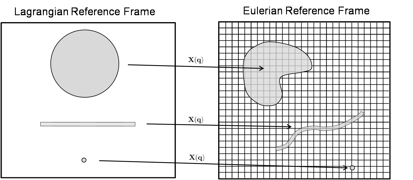
Fig. 1: Stochastic Eulerian Lagrangian Method (SELM) Coupling. In the SELM approach a mixed Eulerian and Lagrangian description is used. The Lagrangian reference frame is used for the particles, extended filaments, and elastic bodies. The Eulerian reference frame is used for the conservation laws (hydrodynamics).

To account for the hydrodynamic coupling of elastic structures, we shall use a variant of the Stochastic Eulerian-Lagrangian Method (SELM), see [2]. Effective equations will be derived for the elastic structures and expressed in terms of the differential operators of the underlying fluid equations. In the limit in which the fluid is treated as having equilibrated to a quasi-steady-state flow, the following effective equations can be derived for the elastic structures accounting for their hydrodynamic interactions and thermal fluctuations

$$\frac{d\mathbf{X}}{dt} = H_{\mbox{\tiny SELM}}\mathbf{F}+\mathbf{g}.$$ (1)

The $\mathbf{F}$ denotes the forces acting on the elastic structure. The $\mathbf{g}$ term accounts for the thermal fluctuations. The effective hydrodynamic coupling tensor $H_{\mbox{\tiny SELM}}=H_{\mbox{\tiny SELM}}(\mathbf{X})$ can be expressed as

$$H_{\mbox{\tiny SELM}} = -\Gamma\wp\mu^{-1}\Delta^{-1}\wp\Lambda.$$ (2)

It will be assumed throughout that $\nabla_{\mathbf{X}}\cdot H_{\mbox{\tiny SELM}}=0$, which ensures phase-space incompressibility in the dynamics of $\mathbf{X}$. For the stochastic dynamics to exhibit fluctuations consistent with statistical mechanics requires the term $\mathbf{g}$ for the thermal fluctuations have a covariance given by [2; 27]

$$G=\langle\mathbf{g}\mathbf{g}^{T}\rangle=2k_{B}{T}H_{\mbox{\tiny SELM}}.$$ (3)

This particular covariance structure can be shown to be a consequence of the principle of detailed balance for an ensemble with the Gibbs-Boltzmann distribution when subject to the stochastic dynamics given by equation 1, see [2].

The effective equations 1–3 can be derived as follows. In the quasi-steady-state limit, the fluid equations can be expressed as

$$\mu\Delta{\mathbf{u}}-\nabla{p} = -\mathbf{f},\hskip 14.22636pt\mathbf{x}\in\Omega$$ (4)

$$\nabla\cdot\mathbf{u} = 0,\hskip 14.22636pt\mathbf{x}\in\Omega$$ (5)

$$\mathbf{u} = 0,\hskip 14.22636pt\mathbf{x}\in\partial\Omega.$$ (6)

The spatial domain occupied by the fluid is denoted by $\Omega$. In the SELM approach [2], the forces acting on the elastic structures are accounted for through a force density acting on the fluid given by

$$\mathbf{f}(\mathbf{x},t)=\Lambda\mathbf{F}.$$ (7)

The $\mathbf{F}$ denotes the collection of forces acting on the elastic structures. The $\Lambda$ denotes the fluid-structure force coupling operator of the SELM approach, see [2].

A key property of which we shall make use is the commutation of the Laplacian operator $\Delta$ and the divergence operator $\nabla\cdot$. This can be expressed as

$$\Delta\left(\nabla\cdot\right)=\left(\nabla\cdot\right)\Delta.$$ (8)

By taking the divergence of equation 4 and using equation 5, we have

$$\Delta{p} = \nabla\cdot\mathbf{f}.$$ (9)

Formally, this has the solution

$$p = -\Delta^{-1}\nabla\cdot\mathbf{f}.$$ (10)

Substituting this for $p$ in equation 4 yields

$$\mu\Delta{\mathbf{u}} = -\wp\mathbf{f}$$ (11)

$$\wp = \mathcal{I}-\left(\nabla\right)\Delta^{-1}\left(\nabla\cdot\right).$$ (12)

The formal solution for $\mathbf{u}$ can be expressed as

$$\mathbf{u} = \wp\mu^{-1}\Delta^{-1}\wp(-\mathbf{f}).$$ (13)

We have used the property that $\wp$ is a projection operator and for solutions $\mathbf{u}$ of equation 4 we have $\wp\mathbf{u}=\mathbf{u}$.

In the SELM approach the dynamics of the elastic structures is given by [2]

$$\frac{d\mathbf{X}}{dt} = \Gamma\mathbf{u}.$$ (14)

The effective stochastic dynamics given by equation 1 for $\mathbf{X}$ is obtained by substituting $\mathbf{u}$ from equation 13 into equation 14 and using equation 7 for $\mathbf{f}$. This derivation uses that the dissipative operator is the Laplacian $\Delta$ which is symmetric, we discuss an alternative form for the effective stochastic dynamics of elastic structures when the dissipative operator is not symmetric in Appendix A.

2.1 Discretization of SELM Hydrodynamic Coupling Tensor

To utilize the SELM hydrodynamic coupling approach in practice requires numerical methods for the approximate computation of the coupling operator $H_{\mbox{\tiny SELM}}$. One approach is provided by discretizing and numerically approximating solutions of the underlying fluid equations.

To facilitate the development of the stochastic numerical methods, it will be convenient to work with numerical discretizations which have a number of special properties. We shall find it convenient to work with linear coupling operators which when discretized satisfy the following adjoint condition

$$\Lambda=\alpha\Gamma^{T}.$$ (15)

Such a condition is closely related to the requirement that the fluid-structure coupling conserves energy, see [2; 25]. For the numerical approximation of the projection operator $\wp$ we shall find it useful for the approximating discretized operator $\tilde{\wp}$ to satisfy $\tilde{\wp}=\tilde{\wp}^{T}$. For the discretized Laplacian we shall require $L=L^{T}$. We shall also find it useful for the $\tilde{\wp}$ to commute with the Laplacian $\tilde{\wp}L=L\tilde{\wp}$. One realization of the SELM approach having these properties is the Stochastic Immersed Boundary Method, see [4; 25]. These conditions are imposed in this initial presentation to avoid a number of technical issues and for clarity in the exposition. In practice, it is likely many of these conditions can be relaxed.

The effective equations for the elastic structures can then be expressed as

$$\frac{d\mathbf{X}}{dt} = \tilde{H}_{\mbox{\tiny SELM}}\left(\mathbf{F}\right)+\mathbf{g}$$ (16)

$$\tilde{H}_{\mbox{\tiny SELM}} = -\Gamma\tilde{\wp}L^{-1}\tilde{\wp}\Lambda.$$ (17)

The $\mathbf{F}$ denotes now the discretized collection of forces acting on the elastic structures. For the discretized model to be consistent with statistical mechanics it is required that

$$G=\langle\mathbf{g}\mathbf{g}^{T}\rangle=2k_{B}{T}H_{\mbox{\tiny SELM}}.$$ (18)

This covariance structure can be found as a consequence of the principle of detailed balance applied to the discretized system, see [2].

3 Generation of the Stochastic Driving Fields Accounting for Thermal Fluctuations

The stochastic driving field $\mathbf{g}$ is required to have the covariance structure

$$G=2k_{B}{T}\tilde{H}_{\mbox{\tiny SELM}}.$$ (19)

Generating random variates with these statistics is in general made challenging since the covariance structure involves correlations which decay like $\sim 1/r$, for the case of three spatial dimensions. Using traditional methods such as Cholesky factorization is expensive. For Cholesky factorization the computational cost scales as $O(M^{3})$, where $M$ is the number of rows in $G$. For systems involving many degrees of freedom, $M$ will be large.

As an alternative approach, we shall generate $\mathbf{g}$ accounting for the thermal fluctuations utilizing the underlying discretized fluid equations. The covariance $G$ can be expressed using the special form of the discretized hydrodynamic coupling operator $\tilde{H}_{\mbox{\tiny SELM}}$ in equation 17. This is given by

$$G = -KL^{-1}K^{T}$$ (20)

$$K = \sqrt{2k_{B}{T}}\Gamma\tilde{\wp}.$$ (21)

A useful consequence of expressing the covariance in this form is that $\mathbf{g}$ can be generated from a Gaussian random field $\boldsymbol{\xi}$ having the covariance structure $C=-L^{-1}$, in the case $L$ is symmetric. We discuss an alternative when $L$ is non-symmetric in Appendix A.

When $L$ is symmetric, equation 20 provides a method for generating $\mathbf{g}$ from

$$\mathbf{g} = K\boldsymbol{\xi}.$$ (22)

The covariance of $\mathbf{g}$ is then given by

$$\langle\mathbf{g}\mathbf{g}^{T}\rangle = K\langle\boldsymbol{\xi}\boldsymbol{\xi}^{T}\rangle K^{T}$$ (23)

$$\langle\boldsymbol{\xi}\boldsymbol{\xi}^{T}\rangle = C=-L^{-1}.$$ (24)

This reduces the problem of efficiently generating $\mathbf{g}$ to the problem of efficiently generating a Gaussian random field $\boldsymbol{\xi}$ with the covariance structure $C=-L^{-1}$. This is challenging in general since the covariance structure is the inverse Laplacian, which has row entries which decay from the diagonal with a scaling like $\sim 1/r$, for the case of three spatial dimensions. In the notation, for the $(i,j)$-entry we take $r=|i-j|\Delta{x}$. For the random field $\boldsymbol{\xi}$, this corresponds to long-range spatial correlations which decay like $\sim 1/r$.

3.1 Stochastic Iterative Methods for Generating Correlated Variates

To generate the random field $\boldsymbol{\xi}$ with the required long-range spatial correlations, we shall exploit the special property of the covariance structure that it is obtained as the inverse of a sparse matrix. As in solving linear systems of equations, this property is suggestive that an iterative approach may be efficient provided we can generalize such iterative methods to the stochastic context. For lattice theories, stochastic iterative methods have been introduced which generalize traditional iterative methods such as SOR, Gauss-Siedel, and Jacobi iterations to generate random fields, see [1; 29]. This was further generalized to obtain stochastic multigrid iterative methods in [14; 13].

For the SELM approach, we shall develop stochastic multigrid iterative methods for generating the random variates $\boldsymbol{\xi}$. This will allow for the efficient generation of the stochastic driving fields $\mathbf{g}$ in the effective hydrodynamic equations for elastic structures given in equation 1 by using equation 22. We now discuss this stochastic iterative approach for generating random variates in more detail.

To generate the stochastic driving fields we shall develop a Gibb’s sampler for the required multi-variate Gaussian distribution. A Gibb’s sampler is developed with stochastic iterations constructed in a manner which exactly preserves the target distribution as an invariant measure of the iterative process. The efficiency of the Gibb’s sampler is determined by two important factors. The first is the computational cost required to compute each iteration of the sampler. The second is the number of iterations required to obtain a random variate having negligible correlations with the previously generated random variates.

For multi-variate Gaussian distributions, we shall use the following linear stochastic iterations

$$\mathbf{Z}^{n+1}=R\mathbf{Z}^{n}+\mathbf{s}+\boldsymbol{\eta}^{n}.$$ (25)

The $\boldsymbol{\eta}^{(n)}$ are taken to be independent Gaussian random variables with mean zero and covariance $J$,

$$\langle\boldsymbol{\eta}^{n}\rangle = 0$$ (26)

$$\langle\boldsymbol{\eta}^{m}(\boldsymbol{\eta}^{n})^{T}\rangle = \delta_{m,n}J.$$ (27)

In the notation, $\delta_{m,n}$ denotes the Kronecker $\delta$-function, the superscript $T$ denotes the vector transpose, $\langle\cdot\rangle$ denotes a probability expectation. The stochastic iteration given in equation 25 can also be expressed in terms of the probability density $\rho^{n}(\mathbf{z})$ at iteration $n$. These probability densities satisfy

$$\rho^{n+1}(\mathbf{z}) = \int\pi(\mathbf{z},\mathbf{w})\rho^{n}(\mathbf{w})d\mathbf{w}$$ (28)

$$\pi(\mathbf{z},\mathbf{w}) = \frac{1}{\sqrt{2\pi\mbox{det}J}}\exp\left[\left(\mathbf{z}-R\mathbf{w}-\mathbf{s}\right)^{T}J^{-1}\left(\mathbf{z}-R\mathbf{w}-\mathbf{s}\right)\right].$$ (29)

We now discuss how a stochastic iterative method having the form of equation 25 can be used to sample a multi-variate Gaussian with a specified mean $\boldsymbol{\mu}$ and covariance $C$. For this purpose, expressions can be derived which relate the iteration matrix $R$ and $\mathbf{s}$ to the mean $\boldsymbol{\mu}$ and covariance $C$, [14; 13]. The mean $\boldsymbol{\mu}$ is given by

$$\boldsymbol{\mu}=(I-R)^{-1}\mathbf{s}.$$ (30)

This follows from equation 25 by taking the expectation of both sides and taking the limit as $n\rightarrow\infty$. The covariance of $\mathbf{Z}^{n+1}$ is given by

$$C^{n+1} = \langle(\mathbf{Z}^{n+1}-\boldsymbol{\mu})(\mathbf{Z}^{n+1}-\boldsymbol{\mu})^{T}\rangle.$$ (31)

This satisfies the following linear recurrence equation

$$C^{n+1}=RC^{n}R^{T}+J.$$ (32)

This follows from equation 31 by using equation 25 to express $\mathbf{Z}^{n+1}$. Taking the limit as $n\rightarrow\infty$ of equation 32 we obtain

$$J=C-RCR^{T}.$$ (33)

This provides a condition on the covariance $J$ for the stochastic driving field which is necessary for the iteration based on $R$ to exhibit the target covariance $C$. A sufficient condition for the invariant measure of equation 25 to be unique can be obtained by re-writing equation 33 as

$$\mathcal{A}C=J.$$ (34)

Retaining the matrix indexing when treating $C$ as a vector, the entries of this operator can be expressed as

$$\mathcal{A}_{(i_{1},i_{2}),(j_{1},j_{2})}=\delta_{i_{1},i_{2}}\delta_{j_{1},j_{2}}-R_{i_{1},j_{1}}R_{i_{2},j_{2}}.$$ (35)

The invariant measure is then ensured to be unique provided the linear operator $\mathcal{A}$ acting on $C$ is non-singular (invertible) in equation 34. This provides a condition on $R$.

We now discuss for a specified mean $\boldsymbol{\mu}$ and covariance $C$ a stochastic iterative scheme for sampling the multi-variate Gaussian. For the given covariance structure $C$, equation 33 gives the required covariance $J$ for the stochastic driving field. To generate the stochastic driving field, we shall find a factor $Q$ so that

$$J=QQ^{T}.$$ (36)

The random variates $\boldsymbol{\eta}$ can then be generated using

$$\boldsymbol{\eta}=Q\boldsymbol{n}$$ (37)

where $\boldsymbol{n}$ is a vector having components which are each independent Gaussians with mean zero and variance one. The computational efficiency of this approach will depend on the particular form of $Q$ and whether a sparse factor can be found satisfying equation 36.

To make this procedure concrete, we shall consider a stochastic sampler based on Gauss-Siedel iterations. In the deterministic setting, the Gauss-Siedel iteration approximates solutions of the following linear system

$$A\mathbf{z}=\mathbf{s}.$$ (38)

The $A$ is assumed to be symmetric. In the Gauss-Siedel iteration, the solution is approximated by splitting the matrix into a diagonal part $D$, upper triangular part $U$, and lower triangular part $L$ so that

$$A=D-L-U.$$ (39)

For symmetric $A$ we have $U=L^{T}$. An iteration of the form of equation 25 is then performed with

$$R=(D-L)^{-1}U.$$ (40)

We now show that a stochastic iterative method can be formulated based on such Gauss-Siedel iterations for sampling a Gaussian with a specified mean $\boldsymbol{\mu}$ and covariance $C=A^{-1}$. As in the deterministic case, the computation of $R\mathbf{z}$ can be performed especially efficiently provided $A=C^{-1}$ is sparse. However, in the stochastic setting it is also required that $Q\boldsymbol{n}$ be computed each iteration, which could be computationally expensive depending on the factor $Q$ of equation 36 which is used.

We now discuss one such approach for obtaining a factor $Q$ satisfying equation 36. For Gauss-Siedel iterations, the covariance $J$ of the stochastic driving term in equation 25 takes the specific form

$$J=QQ^{T}=(D-L-U)^{-1}-(D-L)^{-1}U(D-L-U)^{-1}L(D-L)^{-T}.$$ (41)

An explicit factor for $Q$ can be found [14] and is given by

$$QQ^{T} = (D-L)^{-1}\left[(D-L-U)(D-L-U)^{-1}(D-U)\right.$$

$$\hskip 69.70915pt\left.+\hskip 3.55658ptU(D-L-U)^{-1}(D-L-U)\right](D-U)^{-1}$$

$$= (D-L)^{-1}D(D-U)^{-1}.$$

Since $U=L^{T}$ and the transpose of the inverse is the inverse of the transpose, we have that the following factor $Q$ satisfies equation 41

$$Q = (D-L)^{-1}D^{1/2}.$$ (43)

From this explicit form, we see that $Q$ can be computed efficiently provided $A$ is sparse. This follows since $(D-L)^{-1}$ is a lower triangular matrix whose inverse can be found using back-substitution. The $D$ is the diagonal matrix whose square root is readily computed.

In the case that the covariance $C$ has a sparse inverse, we have that $A=C^{-1}$ is sparse. When $A$ is sparse with a constant number of non-zero entries per row, $Q\mathbf{n}$ can be computed with a computational costs of only $O(N)$, where $N$ is the number of rows of $A$. For $C$ with sparse inverse, one stochastic iteration of the sampler has a total computational cost of only $O(N)$.

The second cost associated with the Gibb’s sampler is the number of iterations required to obtain a new random variate which has a negligible correlation with the previously generated random variates. We now compute the autocorrelation of the random variates generated by the stochastic iterative method given in equation 41. The correlation between the variate generated at iteration $0$ and iteration $k$ is given by

$$C^{(0,k)} = \langle(\mathbf{Z}^{0}-\boldsymbol{\mu})(\mathbf{Z}^{k}-\boldsymbol{\mu})^{T}\rangle.$$ (44)

This can be shown to satisfy the linear recurrence equation

$$C^{(0,k)}=R^{k}C^{(0,0)}.$$ (45)

This follows by using equation 25 to express $\mathbf{Z}^{k}$ in terms of $\mathbf{Z}^{0}$ and $\boldsymbol{\eta}^{j}$ [14].

This indicates that the number of iterations required for the correlations between random variates to become small depends on the initial correlation and the decay rate of the matrix $R$. This provides the following bound in terms of matrix norms

$$\|C^{(0,k)}\|\leq\|R\|^{k}\|C^{(0,0)}\|.$$ (46)

To make more precise what is meant by the correlation becoming negligible between random variates, we shall require the following bound to hold

$$\|C^{(0,k)}\|\leq\epsilon$$ (47)

where $\epsilon$ is small. The number of iterations $k$ required to obtain random variates which have negligible correlation is then bounded below by

$$k\geq\log\left(\epsilon/\|C^{(0,0)}\|\right)/\log\left(\|R\|\right).$$ (48)

This analysis shows there is a direct link between the number of iterations required to obtain a negligible correlation and the number of iterations required in traditional deterministic iterative methods to obtain a high level of accuracy in approximating the solution of a linear system. This suggests that techniques which improve the convergence of traditional iterative methods also should improve the sampling efficiency of stochastic iterative methods. One widely used approach which dramatically improves the convergence of iterative methods is the use of multigrid methods. We explore this approach in detail in the next section.

3.2 Stochastic Multigrid Methods for Generating Correlated Variates

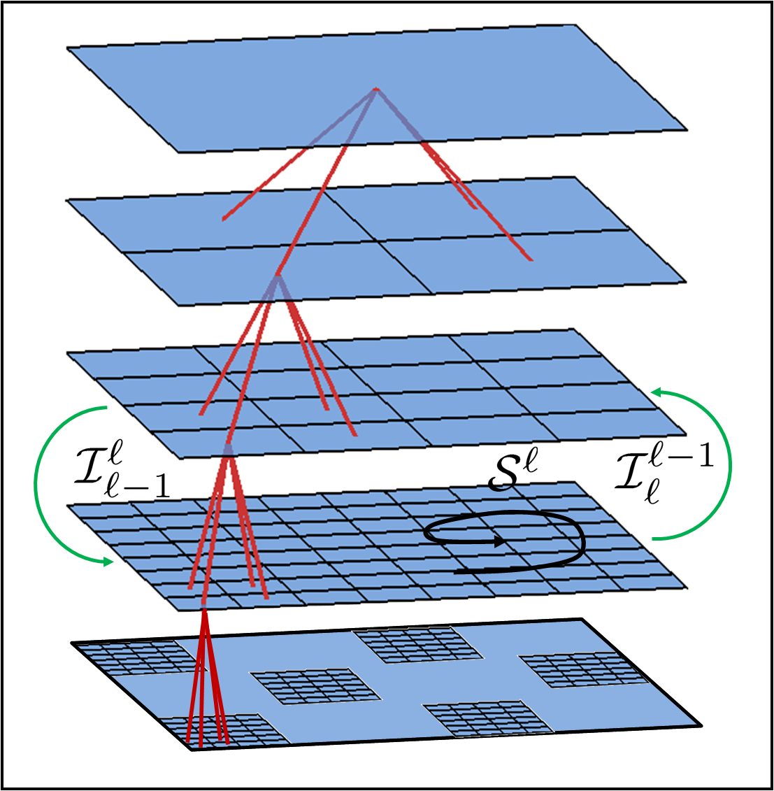
Fig. 2: Multigrid operators. In multigrid, three operators are defined for each level of refinement of the mesh. The first is a smoother operator $\mathcal{S}^{\ell}$ which is used to iteratively approximate the solution of the linear system of equations on the mesh at level $\ell$. For transmission of information between meshes at different levels of resolution, a restriction operator $\mathcal{I}_{\ell}^{\ell-1}$ and a prolongation operator $\mathcal{I}_{\ell-1}^{\ell}$ are defined. The restriction operator $\mathcal{I}_{\ell}^{\ell-1}$ maps data from a more refined mesh at level $\ell$ to data on a less refined mesh at level $\ell-1$. The prolongation operator $\mathcal{I}_{\ell-1}^{\ell}$ maps data from a less refined mesh at level $\ell-1$ to data on a more refined mesh at level $\ell$. These operators are applied in combination to obtain iterations in the multigrid method. For more details, see Algorithms 1,2, and 3.

In the deterministic setting, multigrid can be used to greatly accelerate the convergence of iterative methods [8; 21]. As can be seen from equation 46, reduction in the number of iterations required for convergence in the deterministic setting corresponds to a reduction in the number of iterations required to obtain random variates which are negligibly correlated. We now discuss how the multigrid method can be utilized as a sampler for random variates.

In multigrid iterations three fundamental operators are utilized, see Figure 2. The first is a smoother operator $\mathcal{S}^{\ell}$ which is used to iteratively approximate the linear system of equations on the mesh at level $\ell$. For transmission of information between meshes at different levels of resolution, a restriction operator $\mathcal{I}_{\ell}^{\ell-1}$ and prolongation operator $\mathcal{I}_{\ell-1}^{\ell}$ are defined. The restriction operator $\mathcal{I}_{\ell}^{\ell-1}$ maps data from a more refined mesh at level $\ell$ to data on a less refined mesh at level $\ell-1$. The prolongation operator $\mathcal{I}_{\ell-1}^{\ell}$ maps data from a less refined mesh at level $\ell-1$ to data on a more refined mesh at level $\ell$.

When using multigrid for sampling random variates, the primary modification will be to use a smoothing operator $\mathcal{S}$ which is stochastic. For our present purposes we will take the smoothing operation to be the stochastic Gauss-Siedel iteration defined by equation 25, equation 40, and equation 43. To ensure the target Gaussian with mean $\boldsymbol{\mu}$ and covariance $C$ is the invariant measure of the stochastic multigrid iterations, we shall also require the prolongation operator and restriction operator preserve the variational structure of the linear equations [14]. This variational property is discussed in more detail below.

For the prolongation operator $I_{\ell-1}^{\ell}$in three dimensions we shall use tri-linear interpolation. For the restriction operator we use the adjoint operator given by

$$I_{\ell}^{\ell-1}=\left(I_{\ell-1}^{\ell}\right)^{T}.$$ (49)

This ensures that a consistent variational principle is satisfied for the linear systems of equations associated with each of the levels of resolution used in the multigrid iterations. The variational principle satisfied at the most refined level of the mesh is given by the solution of the linear system of equations being a minimizer of the energy defined by

$$E(\mathbf{v})=\frac{1}{2}\mathbf{v}^{T}A\mathbf{v}-\mathbf{v}^{T}\mathbf{b}.$$ (50)

In the multigrid iterations, the smoother at level $\ell$ approximates the solution of the linear system of equations with

$$A^{(\ell)}\mathbf{v}_{*}^{(\ell)} = \mathbf{b}^{(\ell)}$$ (51)

$$A^{(\ell)} = I_{\ell}^{\ell^{*}}AI_{\ell^{*}}^{\ell}$$ (52)

$$\mathbf{b}^{(\ell)} = I_{\ell}^{\ell^{*}}\mathbf{b}.$$ (53)

Provided condition 49 holds, the solution on the mesh of level $\ell$ is the constrained minimizer of the energy in equation 50 over all vectors of the form $\mathbf{v}=I_{\ell}^{\ell^{*}}\mathbf{v}^{(\ell)}$. This follows since the energy of equation 50 can be expressed as

$$E(I_{\ell}^{\ell*}\mathbf{v}^{(\ell)})=\left(\mathbf{v}^{(\ell)}\right)^{T}A^{(\ell)}\left(\mathbf{v}^{(\ell)}\right)-\left(\mathbf{v}^{(\ell)}\right)^{T}\mathbf{b}^{(\ell)}.$$ (54)

We have used equation 49 to obtain the expression for $A^{(\ell)}$.

This variational property ensures that at each level of refinement the stochastic smoother samples a Gaussian which is the marginal probability distribution of the target multi-variate Gaussian given on the most refined level of the mesh. This follows since for each level of the mesh, the smoother samples the probability distribution

$$\rho^{(\ell)}(\mathbf{v}^{(\ell)})=\frac{1}{\sqrt{2\pi\mbox{det}A^{(\ell)}}}\exp\left[-\frac{1}{2}\left(\mathbf{v}^{(\ell)}\right)^{T}A^{(\ell)}\left(\mathbf{v}^{(\ell)}\right)+\left(\mathbf{v}^{(\ell)}\right)^{T}\mathbf{b}^{(\ell)}\right].$$ (55)

The variational property can be shown to be sufficient to ensure the probability distribution of the target multi-variate Gaussian with mean $\boldsymbol{\mu}$ and covariance $C$ is the invariant measure of the stochastic multigrid iterations [14].

As a basis for our stochastic sampler for random variates, we shall use the formulation of multigrid referred to as ”Fast Adaptive Composite Mesh Multigrid” (abbreviated FAC-multigrid) [22; 15]. The detailed steps of the FAC-multigrid are summarized in Algorithms 1–3. In the case that $A$ is a sparse matrix with only a constant number of non-zero entries per row the FAC-multigrid iterations can be carried-out with a computational cost of $O(N\log(N))$ operations. In the deterministic setting, it can be shown that FAC-multigrid converges with an error with a specified threshold $\epsilon$ in $O(1)$ number of iterations [8; 22; 21]. The stochastic sampler based on FAC-multigrid then provides a method to generate random variates with negligible correlation with a computational cost of only $O(N\log(N))$ operations. Since FAC-multigrid can be used on domains with boundaries and on spatially adaptive meshes, this provides an efficient approach for generating $\boldsymbol{\xi}$ and the stochastic driving term $\mathbf{g}$ in equation 16.

Data: An initial value of $\mathbf{v}$, the right-hand-side $\mathbf{b}$, the number of smoother iterations $(\nu,\mu_{1},\mu_{2})$.

Result: An approximate solution $\mathbf{v}$ of the linear system $A\mathbf{w}=\mathbf{b}$.

Procedure:

1. Compute the residual of the initial value $\mathbf{r}=A\mathbf{v}-\mathbf{b}$.

Initialize the initial value for the correction $\mathbf{q}\leftarrow 0$.

Perform a full sweep of the mesh cells on the multilevel mesh $\mathbf{q}\leftarrow\mbox{Full-Sweep}(\mathbf{q},\mathbf{r},\nu,\mu_{1},\mu_{2})$.

Correct the solution $\mathbf{v}\leftarrow\mathbf{v}+\mathbf{q}$.

Algorithm 1 $\mathbf{v}\leftarrow\mbox{FAC-Multigrid}(\mathbf{v},\mathbf{b},\nu,\mu_{1},\mu_{2})$.

Data: An initial value $\mathbf{q}^{(\ell)}$, the right-hand-side $\mathbf{r}^{(\ell)}$, the number of smoother iterations $(\nu,\mu_{1},\mu_{2})$.

Result: An approximate solution $\mathbf{q}^{(\ell)}$ of the linear system $A^{(\ell)}\mathbf{w}=\mathbf{r}^{(\ell)}$.

Procedure:

1. If the current mesh is at the level of refinement common to all meshes in the hierarchy then perform one V-Cycle on the mesh: $\mathbf{q}^{(\ell)}\leftarrow\mbox{V-Cycle}(\mathbf{q}^{(\ell)},\mathbf{r}^{(\ell)},\mu_{1},\mu_{2})$.

Otherwise, coarsen the residual to the next mesh level $\mathbf{r}^{(\ell-1)}\leftarrow I_{\ell}^{\ell-1}\mathbf{r}^{(\ell)}$.

Perform a full sweep of the cells of the multilevel mesh $\mathbf{q}^{(\ell-1)}\leftarrow\mbox{Full-Sweep}(\mathbf{q}^{(\ell-1)},\mathbf{r}^{(\ell-1)},\nu,\mu_{1},\mu_{2})$.

Apply the correction to the solution on the current level: $\mathbf{q}^{(\ell)}\leftarrow I_{\ell-1}^{\ell}\mathbf{q}^{(\ell-1)}$.

Apply the smoother with the initial value $\mathbf{q}^{(\ell)}$ for $\nu$ iterations for the linear system $A^{(\ell)}\mathbf{w}=\mathbf{r}^{(\ell)}$.

Algorithm 2 $\mathbf{q}^{(\ell)}\leftarrow\mbox{Full-Sweep}(\mathbf{q}^{(\ell)},\mathbf{r}^{(\ell)},\nu,\mu_{1},\mu_{2})$.

Data: An initial value $\mathbf{v}^{(\ell)}$, the right-hand-side $\mathbf{b}^{(\ell)}$, the number of smoother iterations $(\mu_{1},\mu_{2})$.

Result: An approximate solution $\mathbf{v}^{(\ell)}$ of the linear system $A^{(\ell)}\mathbf{w}=\mathbf{b}^{(\ell)}$.

Procedure:

1. Apply the smoother with the initial value $\mathbf{v}^{(\ell)}$ for $\mu_{1}$ iterations for the linear system $A^{(\ell)}\mathbf{w}=\mathbf{b}^{(\ell)}$.

2. If the current mesh is at the coarsest level of refinement in the hierarchy then skip to step 5.

3. Otherwise, perform a V-Cycle on the next coarsest mesh in the hierarchy. Let $\mathbf{b}^{(\ell-1)}\leftarrow I_{\ell}^{\ell-1}\left(\mathbf{b}^{(\ell-1)}-A\mathbf{v}^{(\ell)}\right)$, $\mathbf{v}^{(\ell-1)}\leftarrow 0$, then compute $\mathbf{v}^{(\ell-1)}\leftarrow\mbox{V-Cycle}(\mathbf{v}^{(\ell-1)},\mathbf{b}^{(\ell-1)})$.

Correct the solution on the current level $\mathbf{v}^{(\ell)}\leftarrow\mathbf{v}^{(\ell)}+I_{(\ell-1)}^{\ell}\mathbf{v}^{(\ell-1)}$.

Apply the smoother with the initial value $\mathbf{v}^{(\ell)}$ for $\mu_{2}$ iterations for the linear system $A^{(\ell)}\mathbf{w}=\mathbf{b}^{(\ell)}$.

Algorithm 3 $\mathbf{v}^{(\ell)}\leftarrow\mbox{V-Cycle}(\mathbf{v}^{(\ell)},\mathbf{b}^{(\ell)})$.

4 Spatially Adaptive Discretizations

For many physical systems the level of resolution required to accurately describe the state of the system can vary dramatically over the spatial domain. When approximating such systems numerically, a natural approach is to use discretizations which have different levels of spatial resolution. Many spatially adaptive finite difference discretizations have been developed for this purpose [23; 16; 7; 28; 15].

A significant challenge arising in the stochastic setting for such discretizations is that the discrete Laplacian $L$ is often non-symmetric. The use of symmetry was central in the derivation of the effective equations for the elastic structures satisfying the principle of detailed balance in Section 2. In this report we present initial results for a widely used discretization on adaptive meshes in which the discrete Laplacian $L$ is non-symmetric.

As an alternative approach to obtaining effective stochastic dynamics for the elastic structures, we shall use the stochastic dynamics which would arise for the elastic structures from the fluctuations of the underlying discretized fluid equations with discrete Laplacian $L$ and with a discrete fluctuation-dissipation principle satisfied. This can be shown formally to give the following effective dynamics for the elastic structures (see Appendix A)

$$d\mathbf{X}_{t}=H\mathbf{F}dt+Rd\mathbf{B}_{t}$$ (56)

where

$$H = -\Gamma\wp\alpha\mu^{-1}L^{-1}\wp^{T}\Gamma^{T}$$ (57)

$$RR^{T} = -\Gamma\wp\left(\alpha\mu^{-1}L^{-1}\mathcal{C}+\mathcal{C}L^{-T}\mu^{-1}\alpha\right)\wp^{T}\Gamma^{T}.$$ (58)

In these expressions the operator $L$ is no longer required to be symmetric. The operator $\mathcal{C}$ gives the equilibrium covariance structure of the fluctuations of the fluid velocity consistent with Gibbs-Boltzmann statistics of the discretized system, see [2; 3].

For the equations of hydrodynamics, we shall use a MAC discretization of the Laplacian defined at cell centered nodes on a spatially adaptive structured mesh [23; 15], see Figure 3. To obtain such discretizations on multilevel meshes, we express the Laplacian in terms of the gradient and divergence operators

$$\Delta = \mathcal{D}\mathcal{G}\hskip 14.22636pt\mbox{Laplacian}$$ (59)

$$\mathcal{D} = \nabla\cdot\hskip 14.22636pt\mbox{Divergence}$$ (60)

$$\mathcal{G} = \nabla\hskip 19.91684pt\mbox{Gradient}.$$ (61)

To approximate the operators, we define for any discretization mesh a partition of the spacial domain $\{\Omega_{\mathbf{m}}\}_{\mathbf{m}}$, see Figure 3. For a given partition cell $\Omega_{\mathbf{m}}$ we allow for numerical values to be defined both at the center of the partition cell and at the center of the faces of the partition cell. We approximate the Divergence Operator $\mathcal{D}$ at the center of a partition cell using

$$(D\mathbf{b})_{\mathbf{m}}=\frac{1}{\Delta{x}_{\mathbf{m}}}\sum_{k=1}^{4}\mathbf{b}_{\mathbf{m},k}\cdot\mathbf{n}_{\mathbf{m},k}.$$ (62)

The term $\mathbf{b}_{\mathbf{m},k}$ denotes the vector value at the center of the $k^{th}$ face of the partition cell $\Omega_{\mathbf{m}}$. The $\mathbf{b}$ denotes the composite vector of all such values on the partition. The $\mathbf{n}_{\mathbf{m},k}$ denotes the outward normal to the $k^{th}$ face of the partition cell. The term $\Delta{x}_{\mathbf{m}}$ is the width of the partition cell. The notation $(\cdot)_{\mathbf{m}}$ denotes the component corresponding to the value at the center of the partition cell with index $\mathbf{m}$. A useful property of this approximation to the divergence operator is that its evaluation only requires at the face centers the components in the normal direction, see the dot product in equation 62.

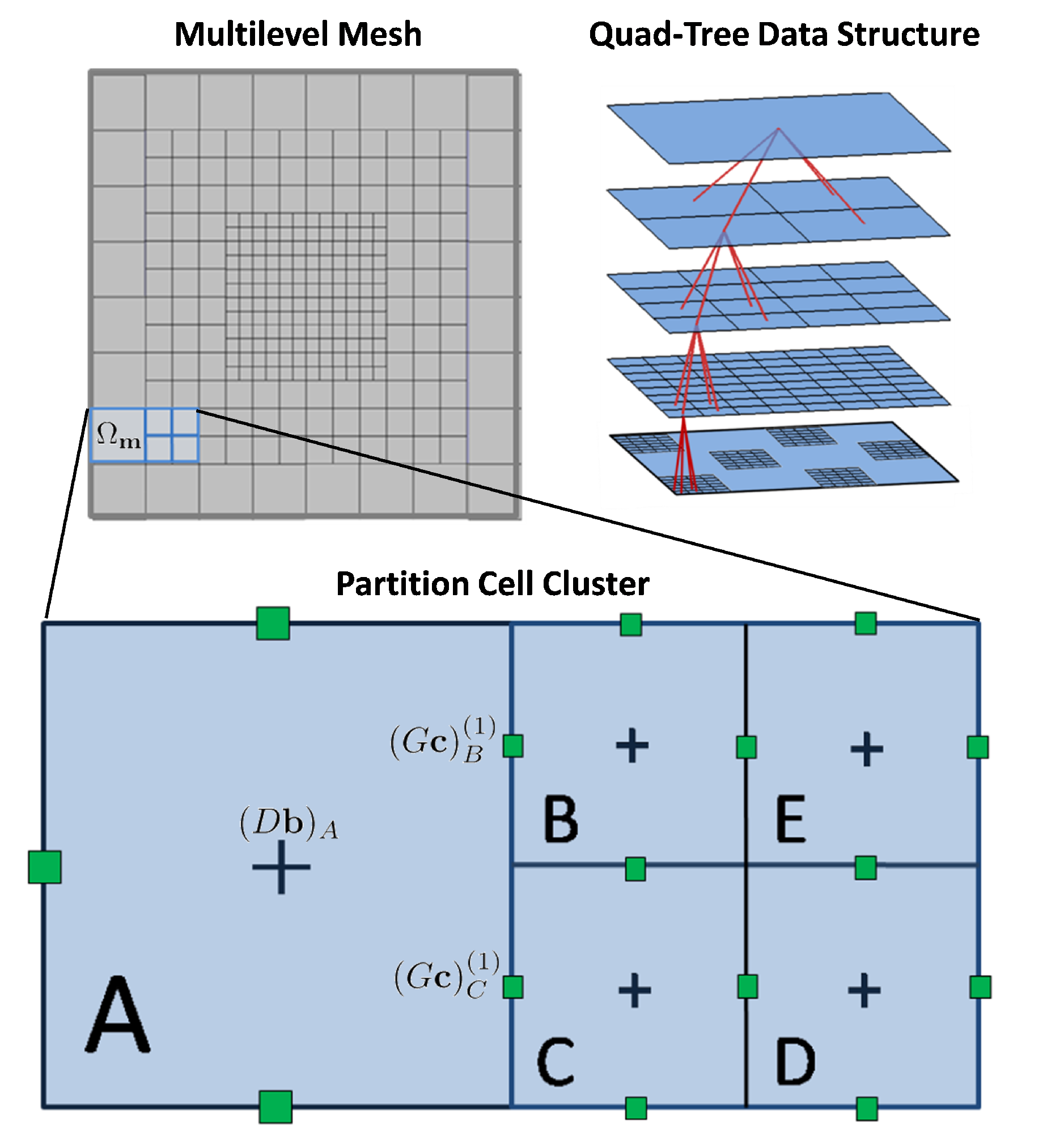
Fig. 3: Mesh Cells at a Typical Coarse-Refined Interface.

We approximate the Gradient Operator $\mathcal{G}$ at the center of the faces of each partition cell. Given the different levels of resolution in the mesh, many cases can arise in principle. By convention, we restrict our methods to deal with meshes which have the nested property that neighboring cells differ in resolution by at most one level. This requires only two cases be considered at each face of a partition cell. The first is when the neighboring cell is at the same level of spatial resolution. This corresponds to $\Delta{x}_{\mathbf{m}}=\Delta{x}_{\boldsymbol{\ell}_{k}}$, where $\boldsymbol{\ell}_{k}$ denotes the index of the neighbor in the direction of the $k^{th}$ face of the partition cell. The second is when the neighboring cells differ by one level of resolution, $\Delta{x}_{\mathbf{m}}=2\Delta{x}_{\boldsymbol{\ell}_{k}}$ or $\Delta{x}_{\mathbf{m}}=\frac{1}{2}\Delta{x}_{\boldsymbol{\ell}_{k}}$.

To approximate the gradient operator on a face shared with a neighbor at the same level of resolution, we use

$$\left(G\mathbf{c}\right)_{\mathbf{m},k}^{(k)} = \mbox{sign}(\mathbf{n}_{\mathbf{m},k}^{(k)})\frac{\mathbf{c}_{\boldsymbol{\ell}_{k}}-\mathbf{c}_{\mathbf{m}}}{\Delta{x}_{\mathbf{m}}}.$$ (63)

In the notation $(\cdot)_{\mathbf{m},k}$ denotes the components corresponding to the vector value at the center of the $k^{th}$ face of the partition cell with index $\mathbf{m}$. The notation $(\cdot)^{(k)}$ denotes the $k^{th}$ vector component. The discrete gradient operator only defines the $k^{th}$ vector component at each face since this is all that is required by the discrete divergence operator $D$ of equation 62.

To approximate the gradient operator on faces shared between neighbors differing by one level of spatial resolution, we must consider a cluster of partition cells. To simplify the discussion, we consider the case where the partition cell with index $\mathbf{m}$ has neighbors at the $k^{th}$ face which are of a more refined level of resolution, $\Delta{x}_{\mathbf{m}}=2\Delta{x}_{\boldsymbol{\ell}_{k}}$. We define the cluster to be the collection of partition cells consisting of the partition cell with index $\mathbf{m}$ (labeled $A$) and the four neighboring partition cells in the direction of the outward normal of the $k^{th}$ face (labeled $B,C,D,E$), see Figure 3. The components of the gradient operator are approximated by

$$\left(G\mathbf{c}\right)_{B}^{(k)} = \mbox{sign}(\mathbf{n}_{\mathbf{m},k}^{(k)})\frac{\frac{1}{2}\left(\mathbf{c}_{B}+\mathbf{c}_{C}\right)-\mathbf{c}_{A}}{\frac{3}{4}\Delta{x}_{\mathbf{m}}}$$ (64)

$$\left(G\mathbf{c}\right)_{C}^{(k)} = \mbox{sign}(\mathbf{n}_{\mathbf{m},k}^{(k)})\frac{\frac{1}{2}\left(\mathbf{c}_{B}+\mathbf{c}_{C}\right)-\mathbf{c}_{A}}{\frac{3}{4}\Delta{x}_{\mathbf{m}}}$$ (65)

$$\left(G\mathbf{c}\right)_{A}^{(k)} = \frac{1}{2}\left[\left(G\mathbf{c}\right)_{B}^{(k)}+\left(G\mathbf{c}\right)_{C}^{(k)}\right].$$ (66)

To obtain a discretization of the Laplacian $\Delta$ on meshes with multiple levels of resolution, we use the approximation

$$L=DG.$$ (67)

The discrete gradient operator $G$ and discrete divergence operator $D$ are defined by equations 62–66. Similar discretizations have been used in [23; 15; 28].

Using this approach to discretize the Laplacian allows for both Neumann and Dirichlet boundary conditions to be imposed readily on rectangular domains. For Neumann conditions the domain is discretized so that faces of the partition cells align with the domain boundary. To impose the Neumann conditions the values of components of the gradient are specified at the center of faces of the partition coinciding with the boundary. For Dirichlet boundary conditions the domain is discretized so that the centers of the partition cells align with the domain boundary. To impose the Dirichlet boundary conditions the values are specified at the center of partition cells coinciding with the boundary. The Laplacian is then computed using equation 67, where the range of the gradient and divergence operators are restricted to the non-boundary values of the partition cells.

5 Performance of the Stochastic Samplers in Practice

We now demonstrate how the stochastic numerical methods perform in practice for generation of the random variates $\boldsymbol{\xi}$. We consider the case of spatially adaptive discretizations, similar results are expected for domains with boundaries. The random variates $\boldsymbol{\xi}$ which are sought are required to have the covariance structure

$$C = \langle\boldsymbol{\xi}\boldsymbol{\xi}^{T}\rangle=-2L^{-1}\mathcal{C}.$$ (68)

The $L$ is the linear operator on the spatially adaptive mesh which approximates the Laplacian differential operator and is no longer required to be symmetric. It can be shown that for the specific spatially adaptive discretization discussed in Section 4 the $L^{-1}\mathcal{C}$ is symmetric. For the purposes of comparison, the stochastic multigrid approach is compared with the stochastic Gauss-Siedel iteration, see Sections 3.1 and 3.2.

As a measure of the efficiency of the generation methods we consider for a given number of iterations the strength of the correlation between random variates generated with each of the stochastic iterative methods. We consider the correlations of random variates for spatial discretizations both in two and three spatial dimensions, see Figure 5. It is found that the stochastic multigrid method greatly reduces the correlations in random variates generated by the stochastic iterative methods. In fact, using stochastic multigrid appears to only require $O(1)$ number of iterations to generate random variates with negligible correlation. The use of Gauss-Siedel stochastic iterations along show a high level of correlations even after many iterations. This is found both for two and three spatial dimensions.

These numerical studies show that the stochastic multigrid method provides a very efficient approach for generating random variates with long-range correlations on spatially adaptive meshes. The presented approach provides a method to generate such random variates with a computational complexity of $O(N\log(N))$ number of operations. This provides a dramatic improvement over Cholesky factorization approaches, which require $O(N^{3})$ operations to generate the factors and $O(N^{2})$ to generate each random variate.

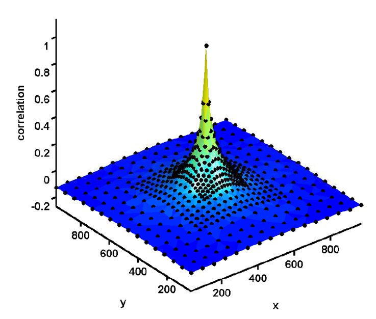
Fig. 4: Covariance structure of the random variates $\boldsymbol{\xi}$ on a spatially adaptive discretization mesh, $-2L^{-1}\mathcal{C}$. An important feature worth noting about the generated variates is the smooth transitions of the covariance over the coarse-refined interfaces. Phenomenological approaches can lead to significant artifacts occurring at such coarse-refined interfaces [3].

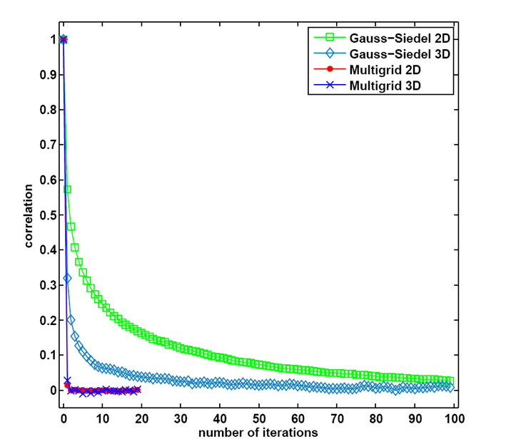
Fig. 5: Comparison of samplers based on Multigrid and Gauss-Siedel. For spatially adaptive meshes in two and three spatial dimensions, a comparison is shown when using the multigrid sampler and Gauss-Siedel sampler. For the multigrid based samplers nearly independent random variates $\boldsymbol{\xi}$ are generated by the stochastic sampler after only a few iterations. For Gauss-Siedel many iterations are required to yield nearly independent random variates $\boldsymbol{\xi}$.

These initial results indicate that the developed stochastic multigrid methods provide a potentially versatile tool for generating the stochastic driving fields in hydrodynamically coupled systems. We have demonstrated here an approach by which stochastic multigrid methods can be developed which allow for the simulation of fluid-structure interactions in the SELM formulation with a computational cost of only $O(N\log(N))$ operations. The developed real-space stochastic numerical methods allow for simulations on spatially adaptive meshes and on flow domains having boundaries. The stochastic numerical method for the stochastic dynamics of elastic structures with SELM hydrodynamic coupling is summarized in Algorithm 4.

Data: Parameters for the physical model and numerical methods.

Result: Stochastic dynamics of the hydrodynamically coupled elastic structures.

Procedure:

1. Compute the forces $\mathbf{F}$ acting on the elastic structures.

Compute the velocity of the elastic structures by evaluating $\tilde{H}_{\mbox{\tiny SELM}}=-\Gamma\tilde{\wp}\alpha L^{-1}\tilde{\wp}\Gamma^{T}$, which uses the discretization of the fluid equations $L$, $\tilde{\wp}$ and the fluid-structure coupling operator $\Gamma$.

Generate the stochastic driving term $\mathbf{g}$ accounting for thermal fluctuations. This is done by using the stochastic multigrid method (Algorithm 1) to generate the random field $\boldsymbol{\xi}$ with covariance $-L^{-1}\mathcal{C}$. The stochastic driving term is generated by $\mathbf{g}=\Gamma\tilde{\wp}\boldsymbol{\xi}$, see equation 22. 4. Update the configuration of the elastic structures using an SDE temporal integrator (i.e. Euler-Maruyama Method).

Return to step 1. to compute the next time step for the dynamics of the elastic structures.

Algorithm 4 Stochastic Dynamics of Elastic Structures with Hydrodynamic Coupling

6 Conclusions

This technical report shows a proof-of-concept approach for efficiently generating the stochastic driving fields in fluid-structure systems using the SELM formalism for hydrodynamic coupling. In future work, a more detailed numerical investigation will be presented demonstrating the efficiency of the presented methods for spatial domains having more complex geometries and for specific discretizations developed for the projection operator on spatially adaptive meshes. Many of the basic ideas presented here are expected to generalize to be applicable more broadly in the development of stochastic numerical methods for the efficient generation of stochastic fields with long-range correlations often required in the simulation of spatially extended stochastic systems.

7 Acknowledgements

The author P.J.A. acknowledges support from research grant NSF DMS-0635535. The author would also like to thank Alexander Roma, Boyce Griffith, and Micheal Minion for helpful suggestions.

Appendix A Derivation of effective stochastic dynamics of elastic structures

We now derive formally a set of effective equations for the dynamics of the elastic structures. The equations only involve the elastic structure degrees of freedom and eliminate the fluid degrees of freedom. For this purpose, we consider increments of the form

$$\Delta\mathbf{X}(t)=\mathbf{X}(t+\Delta{t})-\mathbf{X}(t).$$ (69)

An increment over the time $[t,t+\Delta{t}]$ of the stochastic dynamics for the elastic structures $\mathbf{X}$ is given by

$$\Delta\mathbf{X}=\int_{t}^{t+\Delta{t}}\Gamma\mathbf{u}(q)dq.$$ (70)

In the limit in which the fluid relaxes to a quasi-steady-state on the time scale of the elastic structure dynamics, it is expected that $\mathbf{X}$ will be an Ito or Statonovich stochastic process. Formally, the statistics of this process can be determined by the mean and covariance of its increments [24; 12].

For this purpose, we denote the mean of an increment of $\mathbf{X}$ by

$$\mathbf{a}=\frac{\langle\Delta\mathbf{X}\rangle}{\Delta{t}}.$$ (71)

We denote the covariance of an increment of $\mathbf{X}$ by

$$\mathbf{b} = \langle\left(\Delta\mathbf{X}-\overline{\Delta\mathbf{X}}\right)\left(\Delta\mathbf{X}-\overline{\Delta\mathbf{X}}\right)^{T}\rangle/\Delta{t}$$ (72)

where $\overline{\Delta\mathbf{X}}=\langle\Delta\mathbf{X}\rangle$. A stochastic process for the effective dynamics of $\mathbf{X}$ having increments with approximate mean $\mathbf{a}$ and covariance $\mathbf{b}$ is given by

$$d\mathbf{X}_{t}=\mathbf{a}(t,\mathbf{X}_{t})dt+\boldsymbol{\sigma}(t,\mathbf{X}_{t})d\mathbf{B}_{t}.$$ (73)

where $\boldsymbol{\sigma}\boldsymbol{\sigma}^{T}=\mathbf{b}$. Here we assume an Ito limiting process, but a Statonovich limiting process may also be considered. A more rigorous justification of how to remove the fluid degrees of freedom can be obtained by considering a singular perturbation analysis of the Backward Kolomogorov Equations, see [20].

To determine $\mathbf{a}$ and $\mathbf{b}$, we shall derive formally the leading order expressions in terms of $\epsilon$ and $\Delta{t}$, (with the assumption that $\epsilon\ll\Delta{t}\ll 1$). To simplify the notation we consider the case when $t=0$ without the loss of generality. Throughout, we shall use the approximation

$$\Delta\mathbf{X}=\int_{0}^{\Delta{t}}\Gamma\mathbf{u}(q)dq\approx\Gamma\int_{0}^{\Delta{t}}\mathbf{u}(q)dq.$$ (74)

The solution to the fluid equations can be expressed as

(75)

$$\mathbf{u}(t)=e^{t\epsilon^{-1}\mathcal{L}}\mathbf{u}(0)+\int_{0}^{t}e^{(t-q)\epsilon^{-1}\mathcal{L}}\mathbf{f}(q)dq+\int_{0}^{t}e^{(t-q)\epsilon^{-1}\mathcal{L}}Qd\mathbf{B}_{q}.$$

For the mean, the leading order term is given by

$$\boldsymbol{\alpha} = \Gamma\int_{0}^{\Delta{t}}e^{(t-q)\epsilon^{-1}\mathcal{L}}\mathbf{f}(q)dq$$ (76)

$$= -\Delta{t}\epsilon\Gamma\mathcal{L}^{-1}\mathbf{f}(0)+o(\Delta{t}).$$ (77)

This gives

$$\boldsymbol{a}(t,\mathbf{X}) = -\epsilon\Gamma\mathcal{L}^{-1}\mathbf{f}(0).$$ (78)

We can express the covariance as

$$\langle\left(\Delta\mathbf{X}-\overline{\Delta\mathbf{X}}\right)\left(\Delta\mathbf{X}-\overline{\Delta\mathbf{X}}\right)^{T}\rangle = \Gamma\alpha\Psi\Gamma^{T}$$ (79)

$$\Psi = \int_{0}^{\Delta{t}}dr\int_{0}^{\Delta{t}}ds\phi(r,s)$$ (80)

$$\phi(r,s) = \langle\mathbf{u}(s)\mathbf{u}^{T}(r)\rangle.$$ (81)

Using equation 75 and equation 76, the covariance can be expressed as

$$\Psi = \Psi_{1}+\Psi_{2}$$ (82)

$$\Psi_{1} = \int_{0}^{\Delta{t}}dr\int_{0}^{\Delta{t}}dse^{r\epsilon^{-1}\mathcal{L}}\mathcal{C}(0)e^{s\epsilon^{-1}\mathcal{L}^{T}}$$ (83)

$$\Psi_{2} = \int_{0}^{\Delta{t}}ds\int_{0}^{\Delta{t}}dr\int_{0}^{s}\int_{0}^{r}e^{{\epsilon}^{-1}\mathcal{L}(r-q)}Q\langle d\mathbf{B}_{q}d\mathbf{B}_{w}^{T}\rangle Q^{T}e^{{\epsilon}^{-1}\mathcal{L}^{T}(s-w)}.$$ (84)

The $\mathcal{C}(0)=\langle\mathbf{u}(0)\mathbf{u}^{T}(0)\rangle$ and is independent of $\Delta{t}$ and $\epsilon$. The integral for $\Psi_{1}$ can be performed analytically to obtain

$$\Psi_{1} = \epsilon^{2}\mathcal{L}^{-1}\left(e^{\Delta{t}\epsilon^{-1}\mathcal{L}}-\mathcal{I}\right)\mathcal{C}(0)\left(e^{\Delta{t}\epsilon^{-1}\mathcal{L}^{T}}-\mathcal{I}\right)\mathcal{L}^{-T}.$$ (85)

Under the assumption $\epsilon\ll\Delta{t}$ this gives a leading order term of order $\epsilon^{2}$.

To compute $\Psi_{2}$ we use the Ito Isometry, which can be expressed formally as $\langle d\mathbf{B}_{q}d\mathbf{B}_{w}^{T}\rangle=\delta(q-w)dqdw$. This yields

$$\Psi_{2} = \int_{0}^{\Delta{t}}ds\int_{0}^{\Delta{t}}dr\int_{0}^{s}dw\int_{0}^{r}dq\hskip 3.55658pte^{{\epsilon}^{-1}\mathcal{L}(r-q)}Q\delta(q-w)Q^{T}e^{{\epsilon}^{-1}\mathcal{L}^{T}(s-w)}$$ (86)

$$= \int_{0}^{\Delta{t}}ds\int_{0}^{\Delta{t}}dr\int_{0}^{r\wedge s}dw\hskip 3.55658pte^{{\epsilon}^{-1}\mathcal{L}(r-w)}QQ^{T}e^{{\epsilon}^{-1}\mathcal{L}^{T}(s-w)}$$ (87)

$$= I_{1}+I_{2}$$ (88)

$$I_{1} = \int_{0}^{\Delta{t}}ds\int_{0}^{s}dr\int_{0}^{r}dw\hskip 3.55658pte^{{\epsilon}^{-1}\mathcal{L}(r-w)}QQ^{T}e^{{\epsilon}^{-1}\mathcal{L}^{T}(s-w)}$$ (89)

$$I_{2} = \int_{0}^{\Delta{t}}ds\int_{s}^{\Delta{t}}dr\int_{0}^{s}dw\hskip 3.55658pte^{{\epsilon}^{-1}\mathcal{L}(r-w)}QQ^{T}e^{{\epsilon}^{-1}\mathcal{L}^{T}(s-w)}.$$ (90)

By changing the order of integration we can evaluate $I_{1}$ to obtain

$$I_{1} = \int_{0}^{\Delta{t}}dw\int_{w}^{\Delta{t}}ds\int_{w}^{s}dr\hskip 3.55658pte^{{\epsilon}^{-1}\mathcal{L}(r-w)}QQ^{T}e^{{\epsilon}^{-1}\mathcal{L}^{T}(s-w)}$$ (91)

$$= A_{1}+A_{2}$$ (92)

$$A_{1} = \epsilon\mathcal{L}^{-1}\int_{0}^{\Delta{t}}dw\int_{w}^{\Delta{t}}ds\hskip 3.55658pte^{{\epsilon}^{-1}\mathcal{L}(s-w)}QQ^{T}e^{{\epsilon}^{-1}\mathcal{L}^{T}(s-w)}$$ (93)

$$A_{2} = \epsilon^{2}\mathcal{L}^{-1}QQ^{T}\mathcal{L}^{-T}\left(\epsilon\mathcal{L}^{-T}\left(e^{{\Delta{t}\epsilon}^{-1}\mathcal{L}^{T}}-\mathcal{I}\right)-\Delta{t}\mathcal{I}\right).$$ (94)

Under the assumption $\epsilon\ll\Delta{t}$ we have $A_{2}$ is of order $\epsilon^{2}$.

By changing the order of integration in $A_{1}$, we obtain

$$A_{1} = \epsilon\mathcal{L}^{-1}J_{1}$$ (95)

$$J_{1} = \int_{0}^{\Delta{t}}ds\int_{0}^{s}dw\hskip 3.55658pte^{{\epsilon}^{-1}\mathcal{L}(s-w)}QQ^{T}e^{{\epsilon}^{-1}\mathcal{L}^{T}(s-w)}.$$ (96)

Next, we use that $QQ^{T}=-\epsilon^{-1}\mathcal{L}\mathcal{C}-\mathcal{C}\mathcal{L}^{T}\epsilon^{-1}$, this allows for $J_{1}$ to be expressed as

$$J_{1} = \int_{0}^{\Delta{t}}ds\int_{0}^{s}dw\hskip 3.55658pt\frac{\partial}{\partial{w}}\left[e^{{\epsilon}^{-1}\mathcal{L}(s-w)}\mathcal{C}e^{{\epsilon}^{-1}\mathcal{L}^{T}(s-w)}\right]$$ (97)

$$= \Delta{t}\mathcal{C}-\epsilon\int_{0}^{\epsilon^{-1}\Delta{t}}dr\hskip 3.55658pte^{r\mathcal{L}}\mathcal{C}e^{r\mathcal{L}^{T}}$$ (98)

$$= \Delta{t}\mathcal{C}-\frac{1}{2}\epsilon\mathcal{L}^{-1}\left[e^{\Delta{t}\epsilon^{-1}\mathcal{L}}\mathcal{C}e^{\Delta{t}\epsilon^{-1}\mathcal{L}^{T}}-\mathcal{C}\right].$$ (99)

From equation 95, the leading term when $\epsilon\ll\Delta{t}$ is given by

$$A_{1} = \Delta{t}\epsilon\mathcal{L}^{-1}\mathcal{C}(1+o(1)).$$ (100)

From equation 91, this gives the leading order expression for $I_{1}$

$$I_{1} = \Delta{t}\epsilon\mathcal{L}^{-1}\mathcal{C}(1+o(1)).$$ (101)

A similar analysis can be carried out to show that

$$I_{2} = \Delta{t}\epsilon\mathcal{C}\mathcal{L}^{-T}(1+o(1)).$$ (102)

From equation 82, this shows that to leading order

$$\Psi = \Delta{t}\epsilon\left(\mathcal{L}^{-1}\mathcal{C}+\mathcal{C}\mathcal{L}^{-T}\right)(1+o(1)).$$ (103)

The covariance $\mathbf{b}$ of the increments is then given from equation 79 by

$$\mathbf{b}(\mathbf{X},t) = \epsilon\alpha\Gamma\left(\mathcal{L}^{-1}\mathcal{C}+\mathcal{C}\mathcal{L}^{-T}\right)\Gamma^{T}.$$ (104)

When $\mathcal{L}^{-1}\mathcal{C}$ is symmetric, this simplifies to

$$\mathbf{b}(\mathbf{X},t) = -2\epsilon\alpha\Gamma\mathcal{L}^{-1}\mathcal{C}\Gamma^{T}.$$ (105)

This formal analysis suggests using for the effective stochastic dynamics of the elastic structures

$$d\mathbf{X}_{t}=H\mathbf{F}dt+Rd\mathbf{B}_{t}$$ (106)

where

$$H = -\Gamma\alpha\mu^{-1}\mathcal{L}^{-1}\Gamma^{T}$$ (107)

$$RR^{T} = -\Gamma\left(\alpha\mu^{-1}\mathcal{L}^{-1}\mathcal{C}+\mathcal{C}\mathcal{L}^{-T}\mu^{-1}\alpha\right)\Gamma^{T}.$$ (108)

In the case that $\mathcal{L}=\wp\Delta$ and $\mathcal{C}=k_{B}{T}\delta(\mathbf{x}-\mathbf{y})$ this gives the same effective stochastic dynamics for the elastic structures as equation 1. Since $\wp\Delta=\Delta\wp$ and $\wp\mathcal{C}=\mathcal{C}\wp$, we can express the above operators as

$$H = -\Gamma\alpha\mu^{-1}\wp\Delta^{-1}\wp^{T}\Gamma^{T}$$ (109)

$$RR^{T} = -\Gamma\wp\left(\alpha\mu^{-1}\Delta^{-1}\mathcal{C}+\mathcal{C}\Delta^{-T}\mu^{-1}\alpha\right)\wp^{T}\Gamma^{T}.$$ (110)

For an approximation of the Laplacian $\Delta$ by the discrete operator $L$, this provides the following formal approximation of the operators appearing in the elastic structure equations

$$H = -\Gamma\wp\alpha\mu^{-1}L^{-1}\wp^{T}\Gamma^{T}$$ (111)

$$RR^{T} = -\Gamma\wp\left(\alpha\mu^{-1}L^{-1}\mathcal{C}+\mathcal{C}L^{-T}\mu^{-1}\alpha\right)\wp^{T}\Gamma^{T}.$$ (112)

The utility of this last expression is that it was derived without the assumption that $L$ is symmetric, only that $L$ have negative eigenvalues. The formal derivation provides one approach for obtaining effective stochastic dynamics for the elastic structures from the underlying fluid equations when the discretization of the Laplacian is non-symmetric. As we discuss in Section 4, this is especially important when using discretizations developed for the Laplacian on spatially adaptive meshes which are often non-symmetric.

We should emphasize the above analysis is quite formal. The derivations presented here are meant primarily to motivate the use of the reported stochastic dynamics for the elastic structures. These expressions should be treated with some caution and ultimately need to be established either through a more rigorous analysis or through numerical validation.

References

• [1] Stephenย L. Adler, Over-relaxation method for the monte carlo evaluation of the partition function for multiquadratic actions, Phys. Rev. D, 23 (1981), pp.ย 2901โ€“.
• [2] P.ย J. Atzberger, Stochastic euler-lagrange methods for fluid-structure interactions with thermal fluctuations and shear boundary conditions, (preprint), (2009).
• [3] Paulย J. Atzberger, Spatially adaptive stochastic numerical methods for intrinsic fluctuations in reaction-diffusion systems, Journal of Computational Physics, 229 (2010), pp.ย 3474โ€“3501.
• [4] P.ย J. Atzberger, P.ย R. Kramer, and C.ย S. Peskin, A stochastic immersed boundary method for fluid-structure dynamics at microscopic length scales, Journal of Computational Physics, 224 (2007), pp.ย 1255โ€“1292โ€“.
• [5] A.ย J. Banchio and J.ย F. Brady, Accelerated stokesian dynamics: Brownian motion, Journal of Chemical Physics, 118 (2003), pp.ย 10323โ€“10332โ€“.
• [6] Farida Benmouna and Diethelm Johannsmann, Hydrodynamics of particle-wall interaction in colloidal probe experiments: comparison of vertical and lateral motion, Journal of Physics: Condensed Matter, 15 (2003), pp.ย 3003โ€“.
• [7] M.ย J. Berger and I.ย Rigoutsos, An algorithm for point clustering and grid generation., IEEE Transactions on Systems, Man and Cybernetics, 12(5) (1991), pp.ย 1278โ€“ 1286.
• [8] Williamย L. Briggs, Vanย Emden Henson, and Steveย F. McCormick, A Multigrid Tutorial, Society for Industrial and Applied Mathematics, 2000.
• [9] Y-L. Chen, M.ย D. Graham, J.ย J. deย Pablo, G.ย C. Randall, M.ย Gupta, and P.ย S. Doyle, Conformation and dynamics of single dna molecules in parallel-plate slit microchannels., Phys Rev E Stat Nonlin Soft Matter Phys, 70 (2004), p.ย 060901.
• [10] A.ย J. Chorin, Numerical solution of navier-stokes equations, Mathematics of Computation, 22 (1968), pp.ย 745โ€“&โ€“.
• [11] Jamesย W. Cooley and Johnย W. Tukey, An algorithm for the machine calculation of complex fourier series, Mathematics of Computation, 19 (Apr., 1965), pp.ย 297โ€“301.
• [12] C.ย W. Gardiner, Handbook of stochastic methods, Series in Synergetics, Springer, 1985.
• [13] J.ย Goodman and A.ย D. Sokal, Multigrid monte-carlo method for lattice field-theories, Physical Review Letters, 56 (1986), pp.ย 1015โ€“1018โ€“.
• [14] Jonathan Goodman and Alanย D. Sokal, Multigrid monte carlo method. conceptual foundations, Phys. Rev. D, 40 (1989), pp.ย 2035โ€“.
• [15] B.E. Griffith, Simulating the blood-muscle-valve mechanics of the heart by an adaptive and parallel version of the immersed boundary method., PhD thesis, Courant Institute of Mathematical Sciences, New York University., 2005.
• [16] Louisย H. Howell, John, and Johnย B. Bell, An adaptive-mesh projection method for viscous incompressible flow, SIAM J. Sci. Comput, 18 (1996), pp.ย 18โ€“996.
• [17] Davidย E Huber, Marciย L Markel, Sumita Pennathur, and Kamleshย D Patel, Oligonucleotide hybridization and free-solution electrokinetic separation in a nanofluidic device., Lab Chip, 9 (2009), pp.ย 2933โ€“2940.
• [18] L.ย C. Jellema, T.ย Mey, S.ย Koster, and E.ย Verpoorte, Charge-based particle separation in microfluidic devices using combined hydrodynamic and electrokinetic effects, Lab on a Chip, 9 (2009), pp.ย 1914โ€“1925.
• [19] Xinhui Lou, Jiangrong Qian, Yiย Xiao, Lisan Viel, Arenย E Gerdon, Ericย T Lagally, Paul Atzberger, Theodoreย M Tarasow, Alanย J Heeger, and H.ย Tom Soh, Micromagnetic selection of aptamers in microfluidic channels., Proc Natl Acad Sci U S A, 106 (2009), pp.ย 2989โ€“2994.
• [20] Andrewย J. Majda, Ilya Timofeyev, and Ericย Vanden Eijnden, A mathematical framework for stochastic climate models, Communications on Pure and Applied Mathematics, 54 (2001), pp.ย 891โ€“974.
• [21] Steveย F. McCormick, Multilevel Adaptive Methods for Partial Differential Equations, Society for Industrial and Applied Mathematics, 1989.
• [22] Steveย F. McCormick, Stevenย M. McKay, and J.ย W. Thomas, Computational complexity of the fast adaptive composite grid (fac) method, Applied Numerical Mathematics, 6 (1990), pp.ย 315โ€“327.
• [23] M.ย L. Minion, A projection method for locally refined grids, Journal of Computational Physics, 127(1) (1996), pp.ย 158โ€“178.
• [24] B.ย Oksendal, Stochastic Differential Equations: An Introduction, Springer, 2000.
• [25] C.ย S. Peskin, The immersed boundary method, Acta Numerica, 11 (2002), pp.ย 479โ€“517.
• [26] Christopherย J. Pipe and Garethย H. McKinley, Microfluidic rheometry, Mechanics Research Communications, 36 (2009), pp.ย 110โ€“120.
• [27] L.ย E. Reichl, A Modern Course in Statistical Physics, John Wiley and Sons, 1998.
• [28] Peskinย C.S. Roma, A.M. and M.J. Berger, An adaptive version of the immersed boundary method, J. Comput. Phys., 153 (1999), pp.ย 509โ€“534.
• [29] Charles Whitmer, Over-relaxation methods for monte carlo simulations of quadratic and multiquadratic actions, Phys. Rev. D, 29 (1984), pp.ย 306โ€“.