Circular motion in Reissner-Nordström spacetime

Abstract

We study the motion of neutral test particles along circular orbits in the Reissner-Nordström spacetime. We use the method of the effective potential with the constants of motion associated to the underlying Killing symmetries. A comparison between the black hole and naked singularity cases is performed. In particular we find that in the naked singularity case for $r<Q^{2}/M$ no circular orbits can exist, this radius plays a fundamental role in the physics of the naked singularity. For $r>Q^{2}/M$ and $1<Q/M<\sqrt{9/8}$ there are two stability regions together with a region where all the circular orbits are instable and a zone in which all trajectory are possible but not circular orbits, for $\sqrt{9/8}<Q/M<\sqrt{5}/2$ one stability region and a region where all circular orbits are instable appear, finally for $Q/M>\sqrt{5}/2$ there are all stable circular orbits for $r>Q^{2}/M$.

1 Introduction

We consider the background of a Reissner-Nordström spacetime described in standard spherical coordinates by the line element

$$ds^{2}=-\frac{\Delta}{r^{2}}dt^{2}+\frac{r^{2}}{\Delta}dr^{2}+r^{2}\left(d\theta^{2}+\sin^{2}\theta d\phi^{2}\right)\ ,$$ (1)

where $\Delta=r^{2}-2Mr+Q^{2}$; the horizon radii are given by $r_{\pm}=M\pm\sqrt{M^{2}-Q^{2}}$. The associated electromagnetic potential and field are respectively $A=(Q/r)dt$ and $F=dA=-(Q/r^{2})dt\wedge dr$.

2 The effective potential for neutral test particles

Metric (1) admits the static Killing field $\xi_{t}=\partial_{t}$ and the rotational Killing field $\xi_{\phi}=\partial_{\phi}$. If $p^{a}\equiv\mu u^{a}$ is the four-vector energy momentum of a neutral particle of mass $\mu$, from the Killing vectors and the geodetic motion we obtain two constants of motion related to the Killing vectors, the timelike Killing vector $\xi_{t}$ at infinity related to the stationarity of the metric and the spacelike Killing vector $\xi_{\phi}$ related to the axial symmetry: $E\equiv-g_{\alpha\beta}\xi_{t}^{\alpha}p^{\beta}=\frac{\Delta}{r^{2}}\dot{t}\mu$ is interpreted for time-like geodesics as representing the total energy of the particle as measured by a static observer at infinity, and $L\equiv g_{\alpha\beta}\xi_{\phi}^{\alpha}p^{\beta}=r^{2}\dot{\phi}\mu$ is interpreted as the angular momentum of the particle. From the magnitude $g_{\alpha\beta}p^{\alpha}p^{\beta}=-\mu^{2}$, we find the effective potential for a neutral particle in the background (1) [1]

$$V\equiv\sqrt{\left(1+\frac{L^{2}}{\mu^{2}r^{2}}\right)\left(1+\frac{Q^{2}}{r^{2}}-\frac{2M}{r}\right)}\ .$$ (2)

The energy $E/\mu$ and the angular momentum $L/(\mu M)$ of a (time-like) particle in a circular orbit of radius $r$ are obtained from the condition $\partial V/\partial r=0$ as

$$\frac{E}{\mu}=\frac{\Delta}{r\sqrt{r^{2}-3Mr+2Q^{2}}},\quad\frac{L_{\pm}}{M\mu}=\pm\frac{r\sqrt{r-\frac{Q^{2}}{M}}}{\sqrt{M}\sqrt{r^{2}-3Mr+2Q^{2}}}\ .$$ (3)

2.1 Black holes

In the black hole case $(Q\leq M)$ circular orbits exist for $r>r_{\gamma^{+}}\equiv[3M+\sqrt{(9M^{2}-8Q^{2})}]/2$, where $r=r_{\gamma^{+}}$ represents a photon orbit. The study of the last stable circular orbit ($r_{lsco}$) is sketched in PcEqstab1ma.

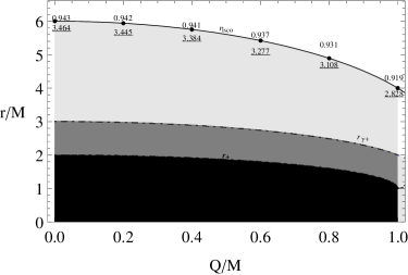
Figure 1: The minimum radius $r_{lsco}/M$ (solid curve) is plotted as a function of the ratio $Q/M$ for the case of black holes, $r_{+}=M+\sqrt{M^{2}-Q^{2}}$ is the outer horizon while the dot-dashed curve is $r_{\gamma^{+}}\equiv[3M+\sqrt{(9M^{2}-8Q^{2})}]/2$. Black regions are forbidden, no trajectories are possible there. In the region inside the curves $r_{+}$ and $r_{\gamma^{+}}$ (gray region) no circular orbits are possible. In the region $r_{\gamma^{+}}$ and $r_{lsco}$, (light-gray region) there are instable circular orbits. Finally for $r>r_{lsco}$ any point represents a stable circular orbit. Numbers close to the selected points represent the value of the energy $E/\mu$ and the angular momentum $L/(\mu M)$ (underlined numbers) of the last stable circular orbits.

In the limiting Schwarzschild case with $Q=0$, we find $r=6M$, as expected. In general, stable orbits are possible only for $r>r_{lsco}$, whereas in the interval $r_{\gamma^{+}}<r<r_{lsco}$ there are only unstable orbits. Moreover, from PcEqstab1ma we conclude that as the charge-mass ratio increases from the Schwarzschild value to the extreme black hole value $(Q=M)$, the radius of the orbit and the corresponding energy and angular momentum of the particle decrease[2, 1, 3, 4].

2.2 Naked singularities

In the naked singularity case $(Q>M)$ circular orbits are possible only for $r\geq r_{*}$, where $r_{*}=Q^{2}/M$ corresponds to the classical radius of a particle with charge $Q$ and mass $M$. For $r=r_{*}$ a time-like “orbit” with $L(r_{*})=0$ (particle at “rest”) and $E/\mu=\sqrt{1-M^{2}/Q^{2}}$ is allowed. For a charge-mass ratio in the interval $M<Q<\sqrt{9/8}M$ there exist time-like circular orbits in the regions $r_{*}<r<r_{\gamma^{-}}$ and $r>r_{\gamma^{+}}$, where $r_{\gamma^{\pm}}\equiv[3M\pm\sqrt{(9M^{2}-8Q^{2})}]/2$. The boundaries $r=r_{\gamma^{\pm}}$ correspond to photon orbits, whereas in the region $r_{\gamma^{-}}<r<r_{\gamma^{+}}$ only space-like circular orbits can exist. For $Q=\sqrt{9/8}M$ time-like circular orbits exist for all $r>r_{*}$, except at the radius $r=(3/2)M$ which corresponds to a photon circular orbit PcEqstab1m(a). Finally, for $Q>\sqrt{9/8}M$ time-like circular orbits can exist for all $r>r_{*}$. As for the stability of the circular orbits, we found that for $M<Q<\sqrt{9/8}M$ there exist stable orbits only in the regions $r_{*}<r<r_{\gamma^{-}}$ and $r>r^{+}_{lsco}$, and unstable orbits are contained in $r_{\gamma^{+}}<r<r^{+}_{lsco}$. For $Q=\sqrt{9/8}M$ all orbits are stable in the region $r>r_{*}$, except at $r=(3/2)M$. For $\sqrt{9/8}M<Q\leq(\sqrt{5}/2)M$, the regions of stability are $r_{*}<r<r^{-}_{lsco}$ and $r>r^{+}_{lsco}$; moreover, orbits in $r^{-}_{lsco}<r<r^{+}_{lsco}$ are unstable. This situation is sketched and summarized in PcEqstab1m(b). Finally, for $Q>(\sqrt{5}/2)M$ all orbits with $r>r_{*}$ are stable. Moreover, as $Q/M$ increases in the interval $[1,\sqrt{5}/2]$, the energy and angular momentum decrease along $r=r^{+}_{lsco}$ and increase along $r=r^{-}_{lsco}$. For the classical radius $r=r_{*}$ the energy increases as $Q/M$ increases. This behavior is summarized in PcEqstab1m(c), see also PcEqstab1mtree. A more detailed discussion of these results will presented elsewhere[2] (see also Refs. Cohen:1979zzb and Liang:1974ha).

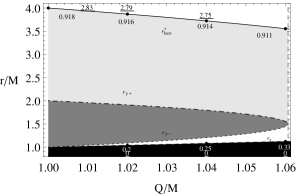
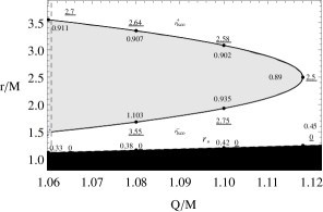
(a)	(b)
(c)

Figure 2: The minimum radius $r^{\pm}_{lsco}/M$ (solid curve) is plotted as a function of the ratio $Q/M$ for the naked singularities. The dashed curve represents the classical radius $r_{*}=Q^{2}/M$ line, the dotted one is $r_{\gamma^{-}}\equiv[3M-\sqrt{(9M^{2}-8Q^{2})}]/2$, while the dot-dashed curve is $r_{\gamma^{+}}\equiv[3M+\sqrt{(9M^{2}-8Q^{2})}]/2$. Black regions are forbidden no trajectories are possible, in the gray regions all trajectories are possible but circular orbits, in the light-gray regions there are instable circular orbits and finally in the white regions there are all stable circular orbits. Numbers close to the selected points represent the value of the energy $E/\mu$ and the angular momentum $L/(\mu M)$ (underlined numbers) of the last stable circular orbits. In (a) region $1<Q/M<\sqrt{9/8}$ is explored. In the region inside the curves $r^{+}_{lsco}$ and $r_{\gamma^{+}}$ (lightgray region) there are instable circular orbits, inside $r_{\gamma^{+}}$ and $r_{\gamma^{-}}$ (Gray region) all trajectories are possible but circular orbits. In $r>r^{+}_{lsco}$ any point represents a stable circular orbit. In (b) region $\sqrt{9/8}<Q/M<\sqrt{5}/2$ is explored. In the region inside the curves $r^{-}_{lsco}$ and $r^{+}_{lsco}$ (lightgray region) there are instable circular orbits, for $Q^{2}/M<r<r^{-}_{lsco}$ and $r>r^{+}_{lsco}$ any point represents a stable circular orbit. Finally in (c) region $Q/M\geq\sqrt{5}/2$ is explored, for $r>r^{*}$ any point represents a stable circular orbit.

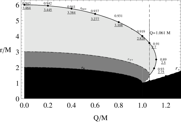
Figure 3: The minimum radius $r^{\pm}_{lsco}/M$ (solid curve) is plotted as a function of the ratio $Q/M$ in the range $[0,1.2]$. The classical radius $r_{*}=Q^{2}/M$, radii $r_{\gamma^{-}}\equiv[3M-\sqrt{(9M^{2}-8Q^{2})}]/2$, $r_{\gamma^{+}}\equiv[3M+\sqrt{(9M^{2}-8Q^{2})}]/2$ and the outer horizons $r_{+}=M+\sqrt{M^{2}-Q^{2}}$ are also plotted. Black regions are forbidden no trajectories are possible, in the gray regions all trajectories are possible but circular orbits, in the light-gray regions there are instable circular orbits and finally in the white regions there are all stable circular orbits. Numbers close to the selected points represent the value of the energy $E/\mu$ and the angular momentum $L/(\mu M)$ (underlined numbers) of the last stable circular orbits.

3 Conclusion

We discussed the motion of neutral test particles along circular orbits in the Reissner-Nordström spacetime. We found that at the classical radius $r=r_{*}=Q^{2}/M$ circular orbits exist with “zero” angular momentum. Inside the classical radius no time-like motion is possible. The difference between black hole and naked singularity configurations was studied in detail. In the case of black holes, the radius of the last stable circular orbit has its maximum value of $r_{lsco}=6M$ in the Schwarzschild limiting case, and reaches its minimum value of $r_{lsco}=4M$ in the case of an extreme black hole $Q=M$. In the case of naked singularities, for a given value of the ratio $Q/M$ two different values of $r_{lsco}$ are possible. As a consequence, a non connected region of stability appears which can exist only in configurations characterized by naked singularities.

References

[1] R.
Ruffini, On the Energetics of Black Holes, Le Astres Occlus
(Les Houches 1972).
[2]
D. Pugliese, H. Quevedo, R. Ruffini (in preparation).
[3] S. Chandrasekhar, The Mathematical Theory of Black
Holes(Oxford University Press, New York, 1983).
[4]
A.N. Aliev, ICTP–report, Trieste, Italy, April 1992.
[5]
J. M. Cohen and R. Gautreau,
Phys. Rev. D 19 (1979) 2273.