Plugs in rough capillary tubes: enhanced dependence of motion on plug length

Abstract

We discuss the creeping motion of plugs of negligible viscosity in rough capillary tubes filled with carrier fluids. This extends Bretherton’s research work on the infinite-length bubble motion in a cylindrical or smooth tube for small capillary numbers $Ca$ Bretherton_1961 (Bretherton 1961). We first derive the asymptotic dependence of the plug speed on the finite length in the smooth tube case. This dependence on length is exponentially small, with a decay length much shorter than the tube radius $R$. Then we discuss the effect of azimuthal roughness of the tube on the plug speed. The tube roughness leads to an unbalanced capillary pressure and a carrier fluid flux in the azimuthal plane. This flux controls the relaxation of the plug shape to its infinite-length limit. For long-wavelength roughness, we find that the above decay length is much longer in the rough tube, and even becomes comparable to the tube radius $R$ in some cases. This implies a much-enhanced dependence of the plug speed on the plug length. This mechanism may explain the catch-up effect seen experimentally Ying_2008 (Ismagilov & Ying).

1 Introduction

The field of multiphase microfluidics has expanded greatly in the last decade because of the numerous applications of the technique in chemistry and biology Gunther_2006 (Gunther & Jensen 2006). Transporting reactants through microchannels in the form of bubbles or droplets has many advantages over the traditional single-phase systems. These include enhanced mixing rate, reduced dispersion and higher interface areas Gunther_2006 (Gunther & Jensen 2006). However there are still many technological problems that remain unsolved. A particular problem that aroused our attention is the control of spacing within a train of long droplets or plugs carried along the channel by a wetting fluid. Such plugs are separated from the tube by a thin lubricating film, whose thickness is controlled by the speed of motion Bretherton_1961 (Bretherton 1961). It is commonly observed Ying_2008 (Ismagilov & Ying) that the separation between the plugs changes as they move. Eventually one plug can coalesce with its neighbor, a process known as the catch-up effect. To our knowledge there is no widely accepted explanation of this effect.

A change in the distance between neighboring plugs is possible only if the fluid flux in the lubricating layer is different in the two plugs. Thus in order to understand the reason for the catch-up effect one needs to analyze the shape and dynamics of this lubricating layer. There are many physical mechanisms that could be responsible for the structure of the lubricating layer. In this work we analyze only one of them: irregularities of the channel shape. We argue that these irregularities, i.e. roughness of the tube wall, could be responsible for the fluctuations of the distance between the plugs. The influence of the substrate geometry or roughness on the lubricating layer thickness has been recognized for several decades and has been studied quite extensively (Stillwagon & Larson (1988); Schwartz & Weidner (1995); Kalliadasis, Bielarz & Homsy (2000); Mazouchi & Homsy (2001); Howell (2003)). In the present work we consider an effect beyond the direct affect on speeds. We find that the roughness enhances dramatically the sensitivity of the thin film width to the plug length, and thus produces speed variations between individual plugs that might eventually lead to catch-up coalescence events.

The earliest discussion of the roughness effect on the plug motion inside capillary tubes dates back to the seminal paper of Bretherton Bretherton_1961 (Bretherton 1961). He suggested that the roughness can be important if its amplitude is comparable to or larger than the lubricating layer thickness. Therefore the roughness effect is usually negligible for large enough tubes where other physical mechanisms are more important (see e.g. Gunther_2006 (Gunther & Jensen 2006), Ajaev_2006 (Ajaev & Homsy 2006) for review). However as modern microfluidic channels become smaller, surface roughness becomes more important relative to the channel width. Probably the first experimental observation that is attributed to the effect of roughness is reported in the work of Chen Chen_1986 (Chen 1986), where deviations from the Bretherton’s predictions were observed for small capillary numbers $Ca$.

On the theoretical side the most widely studied effect of the surface roughness corresponds to the limit where the roughness amplitude is significantly smaller than the lubricating film thickness. In this case the roughness effect can be accounted for via effective boundary conditions: the rough surface can be modeled as a smooth one with non-zero slip length determined by the roughness properties (Einzel, Panzer & Liu (1990); Miksis & Davis (1994); DeGennes (2002)). Krechetnikov and Homsy Krechetnikov_2005 (Krechetnikov & Homsy 2005) have analyzed the effect of the slip length on the lubricating film profile, and showed that the effect is negligible for the slip length smaller than the Bretherton thin film thickness, but leads to a dramatic increase of the lubricating film thickness in the opposite limit: in this case the lubricating film thickness becomes comparable to the slip length and is independent of $Ca$. In a broader context there have been a numerous studies on how the channel geometry affects the dynamics and shape of plugs. Wong et al. (Wong¹ (1995); Wong² (1995)) considered the plug motion in polygonal channels and showed that the shape of the plug strongly depends on the capillary number and that in the limit $Ca\ll 1$, the fluid flux in the lubricating film does not depend on $Ca$. Hazel and Heil Heil_2002 (Hazel & Heil 2002) confirmed this effect by numerical simulations, and showed that a similar behavior is observed in tubes with elliptical cross-sections as well. It should also be noted that the surface roughness can have a non-hydrodynamic effect on the plug motion by changing wetting properties of the surface (Wenzel (1936); Herminghaus (2000); Bico, Tordeux & Quere (2001)) or dynamical destabilization of the lubricating layer due to fluctuations.

In this work we consider capillary tubes with roughness smaller than the lubricating film thickness. In this regime the roughness cannot produce any significant effect on the width of the lubricating layer. However, as we will show, in the rough tube the decay length of the plug shape to its infinite-length limit is increased dramatically. In some cases, the decay length becomes comparable to or even larger than the tube radius. The ripples of the plug shape propagate from the front region to the rear region of the plug, leading to a much-enhanced dependence of the fluid flux on the plug length. On the level of the plug train this effect translates the variations of plug speeds to the fluctuations of the distance between them. Thus it can be responsible for the catch-up events. We also note that this is essentially a non-local effect. To our knowledge this effect has not been discussed perviously.

We will illustrate this effect by using a very simple system, a single air plug of finite length moving through an almost cylindrical tube. For the sake of simplicity, throughout the paper we neglect the effects of gravity, inertia and surfactant concentrations, assuming that the only relevant stresses are due to surface tension and viscosity. We also limit our analysis to the small capillary number regime: $Ca\ll 1$. We assume that the tube roughness can be modeled as weakly non-circular cross sections of the tube, which does not change in the longitudinal direction and can be described by a roughness function $e(\theta)$ with $\theta$ being the azimuthal angle. We will consider the situation where the deformation is smooth enough for the lubrication approximation to be valid, that is, $e(\theta)\ll R\cdot Ca^{2/3}$, i.e. the deformation is small compared to the Bretherton’s thin film thickness. However, we expect that our scaling results can be safely extrapolated to the regime: $e(\theta)\sim R\cdot Ca^{2/3}$.

The structure of this paper is as follows. We start our analysis by revisiting the classical Bretherton solution for the semi-infinite air plug moving in the perfectly cylindrical tube. Then we follow the finite-plug analysis of Teletzke Teletzke_1983 (Teletzke 1983) and extend it to a wider range of plug length. The main finding of this section is the exponential suppression of the speed corrections due to the plug length variations: $\delta U/U\propto\exp\left[-L_{p}/(2L_{\infty})\right]$, where $L_{p}$ measures the length of the plug, and $L_{\infty}=0.643R\cdot(3Ca)^{1/3}$ is the characteristic decay length of the plug shape to its infinite-length limit for the smooth tube case. In Section 3 we explain that the presence of small tube roughness produces a whole spectrum of relaxation modes with different decay lengths $\lambda_{i}$. The relaxation mode with the decay length $\lambda_{max}\simeq L_{p}$ provides the largest contribution to the dependence on the plug length. In Section 4 we estimate of the amplitude of the plug shape distortion due to the roughness. Then we estimate the effect of tube roughness on the finite plug speed in Section 5. We conclude in Section 6 by discussing the limitations of the model and proposing future research directions.

2 Plug speed dependence on the plug length in smooth tubes

Suppose we have a smooth cylindrical capillary tube with radius $R$. It is initially filled with a liquid of viscosity $\mu$, which is called the carrier fluid in the following discussion. Now an air plug with negligible viscosity is forced into the tube and moves slowly together with the carrier fluid due to a pressure gradient along the tube. As discussed in detail later, the plug speed $U$ is different from the speed $V$ of the carrier fluid far away from the plug Jensen_2004 (Hodges, Jensen & Rallison 2004). In this section, we will investigate the effect of the plug length on the plug speed $U$. Both gravitational and inertial effects are assumed to be negligible.

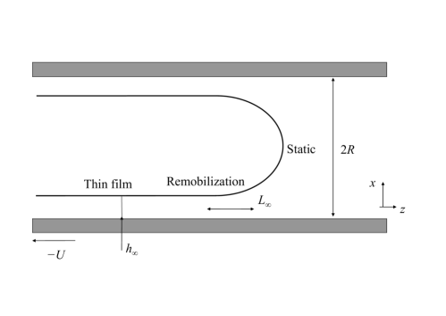
Figure 1: Sketch of a plug identifying Bretherton’s quantities used in the text.

2.1 Bretherton-Teletzke mechanism

In Bretherton’s seminal work Bretherton_1961 (Bretherton 1961), he studied the limit case of semi-infinite air plug motion. He showed that a dimensionless number $Ca$, called capillary number, controls the plug motion:

$$Ca=\frac{\mu U}{\gamma}\,,$$ (1)

where $\gamma$ is an interfacial tension between the plug and the carrier fluid. Bretherton’s steady state solution of a semi-infinite plug is illustrated in Fig.1. For convenience, we have chosen the plug as the frame of reference. In this frame, the tube wall moves with velocity $-U$. The shape of a semi-infinite plug consists of three regions: a spherical cap (static region) is connected to a thin film region of almost constant liquid film thickness $h_{\infty}$ via a transition remobilization region. Since the internal viscosity of the plug is zero, there can be no shear stress at the plug surface. Thus the carrier fluid in the thin film region moves without shear at the wall speed $U$. Bretherton also found that the lubricating film thickness decays exponentially with a decay length $h_{\infty}\,(3Ca)^{-1/3}$, denoted as $L_{\infty}$ Bretherton_1961 (Bretherton 1961). Thus $L_{\infty}$ is a measure of the length of the remobilization region. Both capillary force and viscous force are important in the remobilization region, where the plug shape is determined by an equilibrium between these two forces. In the limit of small capillary numbers, $Ca<0.005\ll 1$, Bretherton derived the dependence of $h_{\infty}$ on $Ca$ and $R$ Bretherton_1961 (Bretherton 1961):

$$h_{\infty}=0.643\,R\cdot(3Ca)^{2/3}\,.$$ (2)

Obviously, both $L_{\infty}$ and $h_{\infty}$ are much less than $R$ for small capillary numbers. Relative motion between the plug and the carrier fluid is governed by an incompressibility constraint. This constraint states that, in the steady state, the total volume of the plug and the carrier fluid between two arbitrary cross sections along the tube doesn’t change over time. Mathematically, it can be translated into the equation: $\pi R^{2}\,V=\pi(R-h_{\infty})^{2}\,U$. By keeping only the lowest order approximation, we get:

$$U/V \simeq 1+2h_{\infty}/R$$ (3)

$$= 1+1.286\,(3Ca)^{2/3}\,.$$

Strictly speaking, Eqn.(3) is only valid in the limit of the semi-infinite plug. For a finite plug, we expect Eqn.(3) to be modified as Teletzke_1983 (Teletzke 1983): $U/V=1+2h^{*}/R$, with $h^{*}$ different from its limiting value $h_{\infty}$. Physically speaking, $-h^{*}$ represents the average carrier fluid flux per unit circumference. As shown in detail later, $h^{*}$ depends on the plug length and approaches $h_{\infty}$ as we increase the length.

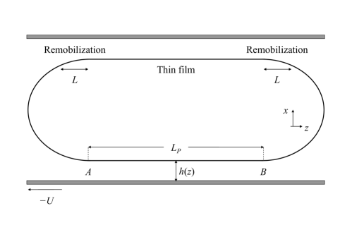
Figure 2: Quantities characterizing a plug of finite length.

The motion of a finite-length air plug in a capillary tube was first studied by Teletzke Teletzke_1983 (Teletzke 1983). In the following discussion length, velocity, and pressure are made dimensionless by using tube radius $R$, plug speed $U$, and capillary pressure $\gamma/R$. Capillary number was kept small in Teletzke’s analysis: $Ca\ll 1$. By imposing a lubrication approximation and appropriate boundary conditions (non-slip condition at the tube wall and stress-free condition at the plug surface), the balance of viscous and capillary pressure gradients yields Teletzke_1983 (Teletzke 1983):

$$\frac{d^{3}h}{dz^{3}}=\frac{3Ca\cdot(h-h^{*})}{h^{3}}\,,$$ (4)

wherever $|dh/dz|\ll 1$. For small $Ca$, this includes both the thin film region and the remobilization region. For a plug of fixed length, $h^{*}$ is a self-consistent parameter whose value is determined by the fact that remobilization regions must match with spherical caps at the plug ends. Suppose the front and rear remobilization regions are separated by a distance $L_{p}$ for a finite plug. Teletzke proposed a method to solve the above differential equation numerically in the limit of short plugs: $L_{p}\lesssim 10L_{\infty}$ Teletzke_1983 (Teletzke 1983). Numerical results obtained by using Teletzke’s method are plotted in Fig.3. As expected, $h^{*}$ approaches $h_{\infty}$ as the plug length increases. However, the trend is not monotonic. The origin of this oscillating behavior will be clear in the next section.

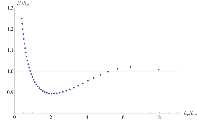
Figure 3: Dependence of $h^{*}$ on the plug length $L_{p}$ obtained by using Teletzke’s method.

Teletzke’s method did not address the asymptotic behavior for finite plugs with length: $L_{p}\gg L_{\infty}$. So the knowledge of the dependence of the plug speed on the plug length is incomplete at the current stage. We only understand two limit cases: Bretherton’s semi-infinite plugs and Teletzke’s short plugs with $L_{p}\lesssim 10L_{\infty}$. In the next section, we complete this previously unstudied part of the plug speed problem, by determining the asymptotic behavior of $h^{*}$ for plugs with large $L_{p}$.

2.2 Asymptotic corrections to the semi-infinite plug speed

Due to rotational symmetry, the problem of determining plug shape is reduced to calculating a lubricating film thickness . The governing equation of $h(z)$ is given by Eqn.(4). For small capillary numbers $Ca$, this differential equation is valid in both the thin film and the remobilization region, as noted above. Its solution has to match spherical caps at the ends of remobilization regions. By using the rescalings: $h=h^{*}\cdot\eta$ and $z=L\cdot\xi$, we may rewrite Eqn.(4) as:

$$\frac{d^{3}\eta}{d\xi^{3}}=\frac{\eta-1}{\eta^{3}}\,.$$ (5)

In the above substitutions, $L$ is the remobilization length of the finite plug defined as: $L\equiv h^{*}\,(3Ca)^{-1/3}$. Comparing with Eqn.(2), we observe that $\eta$ measures thickness in units comparable to the asymptotic thin film thickness $h_{\infty}$. Likewise $\xi$ evidently measures lengths in units comparable to the remobilization length $L_{\infty}$. We denote the plug length $L_{p}$ in these units as $\xi_{p}$. So in this section we will study long plugs with $\xi_{p}\gg 1$.

As we approach the thin film region, $\eta$ becomes arbitrarily close to 1: $|\eta-1|\ll 1$. So we can simplify Eqn.(5) as follows: $d^{3}\eta/d\xi^{3}\simeq\eta-1$. This autonomous equation has solutions of the form: $\eta-1=\exp{(\nu\xi)}$, where $\nu^{3}=1$. It has three roots $\nu_{1}=1$ and $\nu_{2,3}=-1/2\pm\sqrt{3}i/2$, which correspond to three solution modes given below:

$$\psi_{1}(\xi) = \exp{(\xi)}\,,$$

$$\psi_{2}(\xi) = \exp{(-\xi/2)}\,\cos{(\sqrt{3}\xi/2)}\,,$$

$$\psi_{3}(\xi) = \exp{(-\xi/2)}\,\sin{(\sqrt{3}\xi/2)}\,.$$ (6)

So general solutions are linear combinations of these modes, and we have:

$$\eta=1+\sum_{i=1}^{3}C_{i}\psi_{i}(\xi)\,,$$ (7)

where coefficients $C_{i}$ are determined from boundary conditions away from the thin film region. We note for future reference that for large positive $\xi$ , $\eta$ is dominated by the growing $\psi_{1}$ function.

Far from the thin film region treated above, the following relation is valid: $\eta=h/h^{*}\gg 1$. For very small $Ca$, lubrication approximation ($|dh/dz\ll 1|$) is still applicable in this regime Teletzke_1983 (Teletzke 1983). So Eqn.(5) can be approximated as follows: $d^{3}\eta/d\xi^{3}\simeq 0$. Integration of this equation yields parabolic profiles:

$$\eta^{F,R}=\frac{1}{2}P^{F,R}\,\xi^{2}+Q^{F,R}\,\xi+S^{F,R}\,,$$ (8)

where superscripts $F$ and $R$ stand for front and rear solutions, respectively. As defined by Teletzke Teletzke_1983 (Teletzke 1983), axial ($z$-direction) positions of $A$ and $B$ in Fig.2, correspond to axial positions of the lowest points of front and rear parabolas. And he defined the distance between $A$ and $B$ as the plug length $L_{p}$. We will keep Teletzke’s definition in the following discussion.

Since both ends of the plug are spherical caps for small $Ca$, mean curvatures far from the thin film region must match those of spherical caps. As a result, the following constraint needs to be satisfied near the spherical cap: $d^{2}h/dz^{2}=1$. We may rewrite this constraint in terms of reduced variables: $\left.(3Ca)^{2/3}\,(h^{*})^{-1}\cdot d^{2}\eta/d\xi^{2}\right|_{\xi\rightarrow\infty}=1$. By using asymptotic solutions of $\eta$ given in Eqn.(8), we get:

$$\frac{(3Ca)^{2/3}}{h^{*}}\cdot P^{F,R}=1\,.$$ (9)

Since $h^{*}$ is fixed for a given plug, the above equation implies that $P^{F}=P^{R}$. So we can drop the superscript from now on. For a semi-infinite plug, we shall use Bretherton’s result for $h_{\infty}$. This leads to the limit value of $P$ as the plug length goes to infinity: $P_{\infty}=0.643$. As derived in detail in the Appendix of this paper, the dependence of the curvature $P$ on the plug length $\xi_{p}$ for finite long plugs is given by: $P(\xi_{p})=P_{\infty}-1.38\,\delta_{2}(\xi_{p})+0.48\,\delta_{3}(\xi_{p})$, where functions $\delta_{2}$ and $\delta_{3}$ are linear combinations of modes $\psi_{2}$ and $\psi_{3}$, defined in Eqn.(66). By using the constant curvature constraint derived above, we have:

$$\frac{h^{*}}{h_{\infty}} = \frac{P(\xi_{p})}{P_{\infty}}$$ (10)

$$= 1-2.15\,\delta_{2}(\xi_{p})+0.75\,\delta_{3}(\xi_{p})\,.$$

This is the dependence of $h^{*}$ on the dimensionless plug length $\xi_{p}$. It can be easily transformed to represent the dependence on $L_{p}$ via the scaling relation: $L_{p}=\xi_{p}\,P(\xi_{p})\cdot(3Ca)^{1/3}$. Thus the thickness $h^{*}$ oscillates around $h_{\infty}$ with an amplitude that decays as $L_{p}$ increases, and with a decay length of order $L$. Strictly speaking, the above derivation is only valid in the regime: $\xi_{p}\gg 1$, where $\delta_{2}$ and $\delta_{3}$ are arbitrarily small. For illustrative purpose, we extrapolate our analytic results to Teletzke’s short-plug regime and make a comparison between data obtained via two methods in Fig.4. Deviation between two sets of data is obvious for short plugs, where Teletzke’s method is more accurate. For short plugs in the Teletzke’s regime, contributions from all modes are important. Different modes interact nonlinearly, which leads to a much stronger finite-length effect, as shown in Fig.3. Around $L_{p}\sim 6L_{\infty}$ the data obtained via Teletzke’s method begin to merge with our curve. This is the regime where the prediction in Eqn.(10) becomes valid.

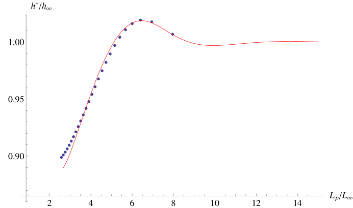
Figure 4: Dependence of $h^{*}$ on the plug length $L_{p}$. Solid line represents our data obtained via a perturbation analysis. Points are data obtained via Teletzke’s method Teletzke_1983 (Teletzke 1983).

In this section, we completed the previously unstudied part of the finite plug speed problem. Together with Teletzke’s method, we can now predict how fast plugs of different length will move in smooth cylindrical tubes. Evidently the speed dependence on the plug length is governed by the solution modes $\psi_{1,2,3}$ in the thin film region. For long plugs studied in this section, their speeds are the most sensitive to the mode with the longest wavelength: $\lambda_{max}\equiv max(|Re(\nu_{i}^{-1})|)$. In smooth tubes, this $\lambda_{max}$ is much smaller than the tube radius $R$ for small capillary numbers of interest. The asymptotic corrections of the finite plug speed is exponentially weak, with a decay length $\lambda_{max}$. For very long plugs with $L_{p}\gg\lambda_{max}$, the speed is almost the same as that of the semi-infinite one. As discussed in the next section, tube roughness can modify the spectrum of solution modes in the thin film region dramatically so that $\lambda_{max}$ may become comparable to or larger than $R$. This is crucial in understanding some interesting experimental phenomena involving the relative motion between finite plugs of different length in non-smooth capillary tubes.

3 Relaxation modes in the thin film region with tube roughness

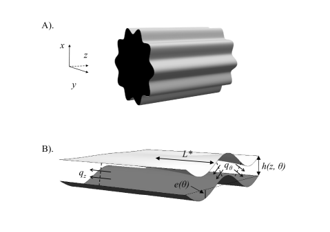
Figure 5: A). A sketch of a capillary tube with azimuthal roughness. B). A plug in the rough tube showing the quantities $e(\theta)$, $h(z,\theta)$, $q_{\theta}$, $L^{*}$ defined in the text.

In this section, we investigate the shape of the thin film region of semi-infinite plugs in tubes with roughness. Here tube roughness is defined as surface deformation of the tube wall, whose shape is not cylindrical. For simplicity, the only type of roughness that we will consider in the following discussion is azimuthal roughness. A tube with the azimuthal roughness preserves its translation symmetry in the axial direction, but cross sections are no longer circular. A sketch of such a tube is plotted in Fig.5(A). The cross section of the rough tube is parameterized in the polar coordinate system as: $\tilde{R}(\theta)=R+e(\theta)$, where $R$ is the smooth tube radius and $\theta$ is the polar angle. The roughness function $e(\theta)$ measures the deformation. In order to isolate the regime of small roughness we may express $e(\theta)$ as: $e(\theta)=\epsilon\,\alpha(\theta)$. Here $\epsilon$ is some small parameter much less than the Bretherton’s thin film thickness $h_{\infty}$, and $\alpha(\theta)$ is a function of order unity. The tube roughness breaks rotational symmetry in the azimuthal plane. As a result, the plug shape now depends on both the $z$ and the $\theta$ coordinate: $h(z,\theta)$. Local lubricating film thickness is defined by the distance between the tube wall and the plug surface: $h(z,\theta)+e(\theta)$, as shown in Fig.5(B). As in the previous section, we nondimensionalize the system by using the smooth tube radius $R$, the plug speed $U$ and the capillary pressure $\gamma/R$. As derived later in this section, the semi-infinite plug shape in the thin film region can be expressed as:

$$h(z,\theta)\simeq H_{\infty}+\sum_{k}C_{k}\,\psi_{k}(\theta)\,\exp{(\nu_{k}z)}\,\,$$ (11)

where $\psi_{k}$ and $\nu_{k}$ are eigenfunctions and eigenvalues governing the relaxation of the plug shape to the cylindrical asymptote $H_{\infty}$. Relaxation mode coefficients $C_{k}$ are determined by boundary conditions away from the thin film region. In Section 4, we will estimate the order of magnitude of $C_{k}$ near the transition between the thin film and the remobilization region.

3.1 The plug shape equation in rough tubes

As in the case of the smooth tube, the plug shape is dictated by the local carrier fluid flux $\vec{q}(z,\theta)$:

$$\vec{q}(z,\theta)=\int_{-e(\theta)}^{h(z,\theta)}\vec{v}(z,\theta,r)\,dr\,,$$ (12)

where $\vec{v}(z,\theta,r)$ is the carrier fluid velocity. As shown in Fig.5(B), $\vec{q}$ has both an axial component $q_{z}$ and an azimuthal component $q_{\theta}$. In the limit of lubrication approximation, and with the same boundary conditions as in the smooth case, these fluxes are given by deGennes_2003 (DeGennes, Brochard & Quere 2003):

$$q_{z} = -(h+e)-\frac{(h+e)^{3}}{3Ca}\,\partial_{z}P\,,$$

$$q_{\theta} = -\frac{(h+e)^{3}}{3Ca}\,\partial_{\theta}P\,,$$ (13)

where $P$ is the capillary pressure on the plug surface. In our reduced units (Howell (2003)): $P=-h-(\partial_{z}^{2}+\partial_{\theta}^{2})h$. Eqn.(13) resembles the usual Poiseuille’s law for thin layer fluid fluxes deGennes_2003 (DeGennes, Brochard & Quere 2003). Rearranging terms in the equation of $q_{z}$, we get:

$$\partial_{z}^{3}h=\frac{3Ca}{(h+e)^{3}}\cdot(q_{z}+h+e)-\partial_{z}\,(1+\partial_{\theta}^{2})h\,.$$ (14)

This is the counterpart of the Teletzke’s plug shape equation, Eqn.(4), in rough tubes. Without roughness, $q_{z}$ is a constant and this equation is sufficient to determine the plug shape $h(z)$. However, $h$ now depends on both $\theta$ and $z$ coordinates, the flux $q_{z}$ is no longer constant and another equation describing the variation of $q_{z}$ is needed to determine the plug shape. This additional equation is the incompressibility constraint: $\partial_{z}q_{z}+\partial_{\theta}q_{\theta}=0$, which leads to the differential equation:

$$\partial_{z}q_{z} = \partial_{\theta}\,\frac{(h+e)^{3}}{3Ca}\,\partial_{\theta}P$$ (15)

$$= -\partial_{\theta}\,\frac{(h+e)^{3}}{3Ca}\,\partial_{\theta}\,\left[(1+\partial_{\theta}^{2})\,h+\partial_{z}^{2}h\right]\,.$$

Combining Eqn.(14) and (15), we get a complete set of differential equations dictating both the plug shape $h$ and the flux $q_{z}$:

$$\left\{\begin{array}[]{lll}\partial_{z}h&=&h^{\prime}\\ \partial_{z}h^{\prime}&=&h^{\prime\prime}\\ \partial_{z}h^{\prime\prime}&=&D^{-1}\cdot(q_{z}+h+e)-(1+\partial_{\theta}^{2})\,h^{\prime}\\ \partial_{z}q_{z}&=&-\partial_{\theta}\,D\,\partial_{\theta}\,\left[(1+\partial_{\theta}^{2})\,h+h^{\prime\prime}\right]\,\,\,\,\,\,\,\,\,\,\,.\end{array}\right.$$ (16)

The first two equations are simply definition equations of variables $h^{\prime}$ and $h^{\prime\prime}$. And the parameter $D$ is given by: $D=(h+e)^{3}/(3Ca)$. Evidently, $z$ and $\theta$ derivatives are separated to two sides of the equation.

In the smooth tube the plug surface has rotational symmetry, so the last equation of Eqn.(16) is simplified as: $\partial_{z}q_{z}=0$. Obviously, it implies a constant flux $q_{z}$. Defining this flux as $-h^{*}$ and using it in the third equation of Eqn.(16), we get:

$$\partial_{z}^{3}h=\frac{3Ca\cdot(h-h^{*})}{h^{3}}-\partial_{z}h\,.$$ (17)

Finally, we saw in the previous section that in the region of interest $h$ varies over a length scale of about $L\sim Ca^{1/3}$. So the slope term $\partial_{z}h$ in Eqn.(17) is negligible compared to the other two terms for small capillary numbers. And the Teletzke’s smooth plug shape equation, Eqn.(4), is obtained after dropping $\partial_{z}h$.

Returning to the case of nonzero $e(\theta)$, for convenience, we define a plug-shape vector: $\vec{\psi}\equiv\left\{h,\,h^{\prime},\,h^{\prime\prime},\,q_{z}+e\right\}^{T}$, where the superscript $T$ indicates the matrix transpose operation. Then we can rewrite the above set of differential equations in a concise matrix form:

$$\partial_{z}\vec{\psi} = \left(\begin{array}[]{cccc}0&1&0&0\\ 0&0&1&0\\ D^{-1}&-(1+\partial_{\theta}^{2})&0&D^{-1}\\ -\partial_{\theta}\,D\,\partial_{\theta}\,(1+\partial_{\theta}^{2})&0&-\partial_{\theta}\,D\,\partial_{\theta}&0\end{array}\right)\,\vec{\psi}$$ (22)

$$\equiv \mathbf{M}(h)\,\vec{\psi}\,.$$ (23)

The nonlinearity of this equation arises because of the dependence of $D$ on $h$. In the following discussion, the roughness function $e(\theta)$ is assumed to be of a simple sinusoidal form:

$$e(\theta)=e_{0}\,\cos{(m\theta)}\,,$$ (24)

where $m$ are positive integers indicating different roughness modes. The roughness amplitude $e_{0}$ is assumed to be small in the regime of interest: $e_{0}\ll h_{\infty}$. As discussed in detail later, Eqn.(23) can be reduced to a linear form in the thin film region. More general roughness functions can be expanded in terms of the Fourier series and analyzed correspondingly.

3.2 Asymptotic shape of semi-infinite plugs

In this section, we consider the asymptotic shape of the front region of a semi-infinite plug of arbitrarily long length $L_{p}\gg 1$. A similar analysis can easily be applied to the rear region of the semi-infinite plug. One immediate concern with these long plugs is that they may be unstable against fission via the Rayleigh instability deGennes_2003 (DeGennes, Brochard & Quere 2003). This instability is independent of the steady state effect that we discuss here. Indeed, for small capillary numbers, the growth rate of the Rayleigh instability becomes negligible deGennes_2003 (DeGennes, Brochard & Quere 2003).

As with the smooth tube case discussed above, we may fix the origin of $z$ coordinate at the transition between the thin film and the remobilization region. Far inside the thin film region where $z\ll-1$, the front semi-infinite plug restores the translation symmetry in the $z$ direction. It implies vanishing $z$ derivatives in this limit, i.e. $\partial_{z}\vec{\psi}(\infty)=0$. Evidently, $h^{\prime}(\infty)$ and $h^{\prime\prime}(\infty)$ are zero. The third equation of Eqn.(23) leads to the condition: $h=-q_{z}-e$. And the asymptotic plug shape $h(\infty)$ is determined by the last equation of Eqn.(23): $-\partial_{\theta}\,D\,\partial_{\theta}\,(1+\partial_{\theta}^{2})h=0$. One obvious solution is that $h(\infty)\equiv H_{\infty}$, where $H_{\infty}$ is a constant. This solution corresponds to a cylindrical plug centered inside the tube. There are two other solutions: $H_{1}\cos\theta$ and $H_{2}\sin\theta$, which correspond to cylindrical plugs shifted laterally inside the tube. The translation symmetry far inside the thin film region leads to the cylindrical plug shape with constant capillary pressure on the plug surface and vanishing flux $q_{\theta}$. For convenience, we focus on the centered asymptote. The implication of non-centered solutions will be addressed in the Discussion section.

The centered solution $H_{\infty}$ measures the magnitude of average $q_{z}$ per unit circumference:

$$\bar{q} \equiv \frac{1}{2\pi}\int_{0}^{2\pi}q_{z}(\infty)\,d\theta$$ (25)

$$= \frac{1}{2\pi}\int_{0}^{2\pi}(-H_{\infty}-e)\,d\theta$$

$$= -H_{\infty}\,.$$

So $H_{\infty}$ has the same physical meaning as $h_{\infty}$ in the smooth tube case, and dictates the relative motion between the plug and the carrier fluid: $U/V=1+2H_{\infty}$. For tubes with small roughness, the difference between $H_{\infty}$ and $h_{\infty}$ is also very small: $|H_{\infty}-h_{\infty}|\ll h_{\infty}$. The leading order correction in $H_{\infty}$ due to the tube roughness appears in the second order of $e$.

3.3 Eigenmodes of relaxation in the thin film region

At finite $z$ values, the semi-infinite plug shape deviates from its cylindrical asymptote. The plug-shape vector $\vec{\psi}$ is rewritten in the following form:

$$\vec{\psi} = \vec{\psi}(\infty)+\delta\vec{\psi}$$ (26)

$$\equiv \left\{H_{\infty}+\delta h,\,\delta h^{\prime},\,\delta h^{\prime\prime},\,-H_{\infty}+\delta q_{z}\right\}^{T}\,,$$

where $\delta\vec{\psi}\equiv\left\{\delta h,\,\delta h^{\prime},\,\delta h^{\prime\prime},\,\delta q_{z}\right\}^{T}$ measures the amount of shape correction. In the thin film region, $\delta\vec{\psi}$ satisfies the relation: $\left|\,\delta\psi^{i}\,\right|<<\left|\,\psi^{i}(\infty)\,\right|$, where the superscript $i$ indicates different vector components. So the plug shape equation (23) can be linearized by using the approximation: $D\simeq D_{1}\equiv(H_{\infty}+e)^{3}/(3Ca)$, and we get:

$$\partial_{z}\delta\vec{\psi} = \left(\begin{array}[]{cccc}0&1&0&0\\ 0&0&1&0\\ D_{1}^{-1}&-(1+\partial_{\theta}^{2})&0&D_{1}^{-1}\\ -\partial_{\theta}\,D_{1}\,\partial_{\theta}\,(1+\partial_{\theta}^{2})&0&-\partial_{\theta}\,D_{1}\,\partial_{\theta}&0\end{array}\right)\,\delta\vec{\psi}$$ (31)

$$\equiv \mathbf{M}_{1}\,\delta{\vec{\psi}}\,,$$ (32)

Evidently, we can solve the above equation via the technique of separation of variables. The general solution of $\delta{\vec{\psi}}$ is given by:

$$\delta{\vec{\psi}}=\sum_{k}C_{k}\,\vec{\psi}_{k}(\theta)\,\exp{(\nu_{k}z)}\,,$$ (33)

where $\vec{\psi}_{k}(\theta)$ and $\nu_{k}$ are eigenvectors and eigenvalues of the matrix operator $\mathbf{M}_{1}$, with $\mathbf{M}_{1}\,\vec{\psi}_{k}(\theta)=\nu_{k}\,\vec{\psi}_{k}(\theta)$. Thus in the thin film region, $\vec{\psi}_{k}(\theta)\,\exp{(\nu_{k}z)}$ are the eigenmodes dictating the relaxation of the plug surface to its cylindrical asymptote. The speed of relaxation is determined by the decay length of each mode $\lambda_{k}$, defined as $\lambda_{k}\equiv|Re(1/\nu_{k})|$. The larger the value of $\lambda_{k}$, the slower of the relaxation process. Relaxation modes with positive $Re(1/\nu_{k})$ are dominant for the front semi-infinite plug. Likewise, negative ones are dominant for the rear semi-infinite plug.

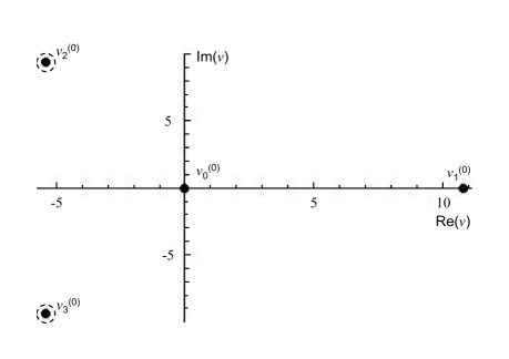
Figure 6: Zeroth harmonic spectrum of the semi-infinite plug shape in the thin film region for tubes with small sinusoidal roughness. Capillary number’s value: $Ca=10^{-3}$.

In the regime of vanishingly small roughness $e(\theta)$, Eqn.(32) can be simplified further as follows:

$$\partial_{z}\delta\vec{\psi} = \left(\begin{array}[]{cccc}0&1&0&0\\ 0&0&1&0\\ D_{0}^{-1}&-(1+\partial_{\theta}^{2})&0&D_{0}^{-1}\\ -D_{0}\,(\partial_{\theta}^{2}+\partial_{\theta}^{4})&0&-D_{0}\,\partial_{\theta}^{2}&0\end{array}\right)\,\delta\vec{\psi}$$ (38)

$$= \mathbf{M}_{0}\,\delta{\vec{\psi}}\,,$$ (39)

where the coefficient $D_{0}$ is now given by: $D_{0}\equiv h_{\infty}^{3}/(3Ca)$. Evidently the matrix operator $\mathbf{M}_{0}$ has no explicit dependence on the $\theta$ coordinate, so its eigenvectors correspond to different harmonics in the Fourier series of $\theta$. Due to the form of the roughness function $e(\theta)$ chosen, we may focus on cosine series solutions with the same symmetry: $\sum C_{n}\cos{(nm\theta)}$. Here $n$ is the harmonic number. Up to the first order in the roughness $e$, we need to analyze the zeroth and first harmonics, with each harmonic leading to four eigenmodes:

$$\delta\vec{\psi} \simeq \delta\vec{\psi}^{(0)}+\delta\vec{\psi}^{(1)}$$ (40)

$$= \sum_{k=0}^{3}C_{k}^{(0)}\,\vec{\psi}_{k}^{(0)}\,\exp{(\nu_{k}^{(0)}z)}+\sum_{k=1}^{4}C_{k}^{(1)}\,\vec{\psi}_{k}^{(1)}\cos{(m\theta)}\,\exp{(\nu_{k}^{(1)}z)}\,,$$

where superscripts (0) and (1) stand for the zeroth and the first harmonics respectively. The zeroth harmonic solution $\delta\vec{\psi}^{(0)}$ preserves the rotational symmetry and satisfies the equation:

$$\partial_{z}\delta\vec{\psi}^{(0)}=\left(\begin{array}[]{cccc}0&1&0&0\\ 0&0&1&0\\ D_{0}^{-1}&-1&0&D_{0}^{-1}\\ 0&0&0&0\end{array}\right)\,\delta\vec{\psi}^{(0)}\,.$$ (41)

The above matrix operator is a four-by-four matrix and does not depend on the form of the roughness function. So the zeroth harmonic spectra of different roughness functions are the same. For small capillary numbers, four eigenvalues of this matrix $\nu_{k}^{(0)}$ are given by: $\nu_{0}^{(0)}=0$, $\nu_{1}^{(0)}=D_{0}^{-1/3}$, $\nu_{2}^{(0)}=D_{0}^{-1/3}(-1/2+i\sqrt{3}/2)$, and $\nu_{3}^{(0)}=D_{0}^{-1/3}(-1/2-i\sqrt{3}/2)$. There is no plug surface relaxation associated with the mode $\nu_{0}^{(0)}$. It corresponds to the degree of freedom to fix the radius of the cylindrical asymptote as $z\rightarrow\infty$. The other three modes $\nu_{1}^{(0)}$, $\nu_{2}^{(0)}$ and $\nu_{3}^{(0)}$ correspond to the ones found in the previous section for the smooth tube, up to a difference in the choice of units. For illustrative purpose, the zeroth harmonic spectrum is plotted in Fig.6. Obviously, $\nu_{2}^{(0)}$ and $\nu_{3}^{(0)}$ are the relaxation modes with the longest decay length $\lambda_{max}^{(0)}$ in this spectrum.

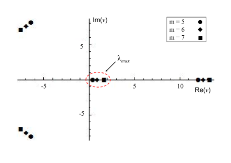
Figure 7: First harmonic spectrum of the semi-infinite plug shape in the thin film region for tubes with small sinusoidal roughness. Cases with $m=$5, 6, 7 are plotted. Capillary number’s value: $Ca=10^{-3}$.

A major difference between the rough tube and the smooth one comes from the first harmonic solution $\delta\vec{\psi}^{(1)}$. It satisfies the equation:

$$\partial_{z}\delta\vec{\psi}^{(1)}=\left(\begin{array}[]{cccc}0&1&0&0\\ 0&0&1&0\\ D_{0}^{-1}&-1+m^{2}&0&D_{0}^{-1}\\ D_{0}\,(m^{2}-m^{4})&0&D_{0}\,m^{2}&0\end{array}\right)\,\delta\vec{\psi}^{(1)}\,.$$ (42)

Four eigenvalues are solutions of the characteristic equation:

$$\nu^{4}+(1-2m^{2})\,\nu^{2}-D_{0}^{-1}\,\nu+m^{4}-m^{2}=0\,.$$ (43)

The first harmonic spectra with the roughness mode number $m=$5, 6, and 7 are plotted in Fig.7. Compared to the zeroth harmonic spectrum shown in Fig.6, the mode with the longest decay length $\lambda_{max}^{(1)}$ now lies near the origin and has much longer decay length. For small values of $m$, i.e. long wavelength roughness, $\lambda_{max}^{(1)}$ becomes comparable to or even larger than the tube radius $R$. Obviously, $\lambda_{max}^{(1)}>\lambda_{max}^{(0)}$ in the regime of interest. So $\lambda_{max}^{(1)}$ is the new slowest decay mode in rough tubes after analyzing both the zeroth and the first harmonic spectra. So we will drop the superscript $(1)$ and refer to it as $\lambda_{max}$ from now on.

To better understand the origin of these slow relaxation modes in tubes with roughness, we propose a following physical explanation of $\lambda_{max}$. The remobilization region ends at about distance $z\sim L_{\infty}$ from the spherical cap. At this transition between the remobilization region and the thin film region, the plug shape has not reached its cylindrical asymptote yet. We assume that the plug surface has a typical height variation of about $\Delta h$. A sketch of such a plug cross section is given in Fig.5(B). Non-cylindrical plug shape leads to unbalanced capillary pressure $P$ in the azimuthal plane and a non-zero lateral flow $q_{\theta}$. In the thin film region, the plug surface relaxes toward the cylindrical asymptote via this flow $q_{\theta}$. Suppose that the relaxation length scale is given by $L^{*}$. It can be estimated as the product between the carrier fluid speed $U$ in this region and a relaxation time scale $T$ over which $q_{\theta}$ smoothes the plug surface. In the following analysis, we will estimate the length scale $L^{*}$ and obtain its scalings with other system parameters. For this part of discussion only, we will work in the lab units.

The expression of the lateral flux $q_{\theta}$ is given by Eqn.(13). In the lab units, we have:

$$q_{\theta}=-\frac{(h+e)^{3}}{3\mu R}\,\partial_{\theta}P\,.$$ (44)

As mentioned above, the capillary pressure $P$ is no longer a constant in the azimuthal plane for the non-cylindrical plug shape. The length scale in the $\theta$ direction is defined by the roughness wavelength $l_{\theta}\sim R/m$. So we may estimate $\theta$ derivatives as: $R^{-1}\,\partial_{\theta}h\sim(m/R)\cdot\Delta h$. Since the $z$-direction plug surface adjustment mostly happens in the remobilization region, we expect that $\theta$ derivatives are typically much larger than $z$ derivatives in the thin film region. The limit of this assumption will be derived later. So the capillary pressure $P$ is approximated as follows:

$$P = -\gamma\,\left[\,\partial_{z}^{2}h-\,\frac{(1+\partial_{\theta}^{2})h}{R^{2}}\right]$$ (45)

$$\sim \gamma\,\frac{\Delta h}{(R/m)^{2}}\,.$$

By definition, the surface relaxation time scale $T$ is given by:

$$T\simeq\frac{\Delta h}{R^{-1}\,\partial_{\theta}q_{\theta}}\sim\frac{\mu\,(R/m)^{4}}{\gamma\,h_{\infty}^{3}}\,.$$ (46)

The relaxation length scale $L^{*}$ is estimated as the product between $U$ and $T$: $L^{*}\sim Ca\,R^{4}/(h_{\infty}^{3}\,m^{4})$. We may simplify this estimation of $L^{*}$ further by using the scaling of $h_{\infty}$ and get:

$$L^{*}\sim\frac{R}{Ca\cdot m^{4}}\,.$$ (47)

For a self-consistent derivation, $m$’s value is constrained by the approximation used in Eqn.(45). This is equivalent to the condition: $R^{-1}\,\partial_{\theta}h\gg\partial_{z}h$, which yields the relation: $l_{\theta}\ll L^{*}$. By using the estimation of $L^{*}$ obtained above, we get the valid regime of the roughness mode number: $m\ll Ca^{-1/3}$. It corresponds to capillary tubes with long wavelength roughness. Obviously $L^{*}$ is much longer than the smooth remobilization length $L_{\infty}$ in this regime of roughness.

The length scale $L^{*}$ is actually the longest decay length $\lambda_{max}$ in the eigenvalue spectrum derived previously. It corresponds to the smallest solution of Eqn.(43), which goes to zero as $Ca$ approaches zero. For this root, the $D_{0}^{-1}\,\nu$ term dominates the higher power terms of $\nu$, and Eqn.(43) simplifies as follows:

$$-D_{0}^{-1}\cdot\lambda_{max}^{-1}+m^{4}-m^{2}=0\,.$$ (48)

For an order of magnitude estimation, we may drop the term $m^{2}$ relative to $m^{4}$ and get: $\lambda_{max}\sim Ca/(h_{\infty}^{3}\,m^{4})$. This is the same scaling relation as that of $L^{*}$, up to a difference in the choice of units. Thus $L^{*}$ and $\lambda_{max}$ measure the same length scale in rough tubes. The scaling argument presented above physically explains the origin of large $\lambda_{max}$ values in the rough tube. This new length scale reflects the slow relaxation of the plug shape via a vanishingly small lateral fluid flux $q_{\theta}$. Historically, people has observed some evidence of this new length scale in non-cylindrical tubes Wong¹ (1995).

4 Amplitude of the plug surface bumpiness in the remobilization region

In the previous section, we analyzed the semi-infinite plug shape in the thin film region and found that the plug surface decays to its cylindrical asymptote via different relaxation modes. To proceed further, we must understand how the rough tube wall imposes a non-cylindrical plug shape in the first place. For small roughness, the plug shape is dominated by the zeroth and the first harmonic solutions:

$$h(z,\theta)\simeq H_{\infty}+\sum_{k=1}^{3}C_{k}^{(0)}\,\exp{(\nu_{k}^{(0)}z)}+\sum_{k=1}^{4}C_{k}^{(1)}\,\cos{(m\theta)}\,\exp{(\nu_{k}^{(1)}z)}\,,$$ (49)

where the coefficients $C_{k}^{(0)}$ and $C_{k}^{(1)}$ are determined from the boundary conditions away from the thin film region. In this section, we will treat the front and the rear semi-infinite plugs simultaneously, with the understanding that only the modes with the correct sign of $Re(1/\nu_{k})$ are excited for a single semi-infinite plug. The $z$ coordinate origin is fixed at the transition between the thin film and the remobilization region as in Section 2. In that section we have shown that the zeroth harmonic coefficients $C_{k}^{(0)}$ are of the order of $h_{\infty}$. We will see later in this section that the first harmonic coefficients $C_{k}^{(1)}$ are of the order of $e_{0}$. The exact numerical solutions will be presented in our future work.

In the remobilization region, the governing equation of the plug shape $h(z,\theta)$ is derived by combining the last two equations in Eqn.(16):

$$\partial_{z}(h+e)-\frac{1}{3Ca}\left[\partial_{z}(h+e)^{3}\partial_{z}+\partial_{\theta}(h+e)^{3}\partial_{\theta}\right](1+\partial_{z}^{2}+\partial_{\theta}^{2})h=0\,.$$ (50)

This equation can be simplified further by noticing the fact that in the remobilization region, $h$ varies over about $(3Ca)^{1/3}$ in the $z$ direction and about $m^{-1}$ in the $\theta$ direction. For long wavelength roughness with $m\ll(3Ca)^{-1/3}$, the following estimation of derivatives is valid : $\partial_{z}h\gg\partial_{\theta}h$. In other words, in the remobilization region the plug shape $h(z,\theta)$ varies much more rapidly in the $z$ direction than in the $\theta$ direction. So we may keep only $z$ derivatives in Eqn.(50), and get:

$$\partial_{z}h=\frac{1}{3Ca}\left[\partial_{z}(h+e)^{3}\partial_{z}^{3}\,\right]h\,.$$ (51)

Bretherton’s smooth tube solution $h_{0}(z)$ satisfies the above differential equation with $e=0$. In the regime of small roughness, Eqn.(51) can be solved perturbatively by expanding around the smooth tube solution $h_{0}(z)$: $h(z,\theta)=h_{0}(z)+u^{(0)}(z)+u^{(1)}(z)\,\cos(m\theta)$. Here $u^{(0)}$ and $u^{(1)}$ are the leading order plug shape correction attributed to the tube roughness. For vanishingly small roughness, the relation $|u^{(0,1)}/h_{0}|\ll 1$ holds for arbitrary $z$. Since we are interested in the coefficients of the first harmonic solution, we will focus on the shape correction $u^{(1)}$ for the rest of this section. Keeping only the lowest order approximation, $u^{(1)}$ satisfies the following equation:

$$\left(\partial_{z}h_{0}^{3}\,\partial_{z}^{3}\right)u^{(1)}+(3h_{0}^{2}\,\partial_{z}^{3}h_{0}-3Ca)\,\partial_{z}u^{(1)}+\left[\partial_{z}(3h_{0}^{2}\,\partial_{z}^{3}h_{0})\right](u^{(1)}+e_{0})=0\,.$$ (52)

This is an inhomogeneous differential equation. The correct boundary conditions of $u^{(1)}$ are that it goes to zero as $z$ approaches the spherical cap, and matches the relaxation modes in Eqn.(49) as $z$ approaches the thin film region. The general solution of Eqn.(52) takes the form: $u^{(1)}(z)=e_{0}\left(f(z)-1\right)$. Here $f(z)$ is a dimensionless function satisfying the homogeneous equation and goes to 1 as $z$ approaches the spherical cap. By using the rescalings as in the smooth tube: $h_{0}=h_{\infty}\cdot\eta_{0}$, and $z=L_{\infty}\cdot\xi$, we get the following equation of $f$:

$$\left(\partial_{\xi}\eta_{0}^{3}\,\partial_{\xi}^{3}\right)f+(3\eta_{0}^{2}\,\partial_{\xi}^{3}\eta_{0}-3)\,\partial_{\xi}f+\left[\partial_{\xi}(3\eta_{0}^{2}\,\partial_{\xi}^{3}\eta_{0})\right]f=0\,.$$ (53)

After the rescaling both $\eta_{0}$ and its $\xi$ derivatives are of the order of unity in the remobilization region, so all coefficients in Eqn.(53) are of the order of unity. Together with the boundary condition of $f$ near the spherical cap, the solution $f(z)$ must be of the order of unity in the remobilization region. By matching with relaxation modes in the thin film region, we get an order of magnitude estimation of the first harmonic coefficients: $C_{k}^{(1)}\simeq e_{0}$. Thus the semi-infinite plug shape in the thin film region can be rewritten as follows:

$$h(z,\theta)\simeq H_{\infty}\,\left(1+\sum_{k=1}^{3}\tilde{C}_{k}^{(0)}\,\exp{(\nu_{k}^{(0)}z)}\right)+\sum_{k=1}^{4}\tilde{C}_{k}^{(1)}\,e(\theta)\,\exp{(\nu_{k}^{(1)}z)}\,,$$ (54)

where all coefficients $\tilde{C}_{k}^{(0)}$ and $\tilde{C}_{k}^{(1)}$ are of the order of unity. The above estimation is valid for both the front and the rear semi-infinite plug.

5 Finite plug motion in rough tubes

In this section, we qualitatively study the dependence of the finite plug motion on the plug length in the rough tube, following the logic of Section 2. For the finite plugs, relaxation modes of both signs of $Re(1/\nu_{k})$ are excited in the thin film region. Far inside the thin film region where the plug shape is almost cylindrical, all the other relaxation modes are vanishingly small compared to the slowest decay mode $\lambda_{max}$. Thus we may focus on the effect of $\lambda_{max}$. By defining a $\tilde{z}$ coordinate whose origin is at some position far inside the thin film region, the plug shape is approximated as follows:

$$h(z,\theta)\simeq H_{\infty}+\tilde{C}\,e(\theta)\,\exp{\left[(\tilde{z}-\ell)/\lambda_{max}\right]}\,,$$ (55)

where $\tilde{z}\equiv z+\ell$. The coefficient $\tilde{C}$ is of the order of unity as derived in the previous section. Here the variable $\ell$ measures the half length of the finite plug. For plugs used in microfluidic experiments, $\ell$ is usually comparable to or larger than the tube radius $R$ Ying_2008 (Ismagilov & Ying). As mentioned previously, the relative motion between the plug and the carrier fluid is governed by the azimuthal average of $q_{z}$:

$$U/V = 1-\frac{1}{\pi}\int_{0}^{2\pi}q_{z}\,d\theta$$ (56)

$$= 1-2\bar{q}\,.$$

Far inside the thin film region, the plug shape is almost cylindrical, which leads to the following estimation of the carrier fluid fluxes: $q_{z}\simeq-h-e$, and $q_{\theta}\simeq 0$. By using the approximate plug shape in Eqn.(55), we have: $q_{z}(z,\theta)\simeq-H_{\infty}-\tilde{C}\,e(\theta)\,\exp{\left[(z-\ell)/\lambda_{max}\right]}-e(\theta)$. Evidently, the average flux $\bar{q}$ vanishes in this linear approximation. Thus any effect on $\bar{q}$ appears in the second or higher order of the roughness: $\bar{q}+H_{\infty}=\tilde{B}\,e_{0}^{2}\,\exp(-2\ell/\lambda_{max})+O(e_{0}^{4})$. The asymptotic dependence of the plug speed on the plug length is exponentially small for long plugs, and we have:

$$U/V\simeq 1+2H_{\infty}\,\left[1+\frac{\tilde{B}\,e_{0}^{2}}{H_{\infty}}\,\exp(-2\ell/\lambda_{max})\right]\,.$$ (57)

The above form of length dependence implies an interesting resonance effect in the rough tube. To illustrate this effect, we may estimate the speed difference between two plugs with length $\ell_{1}$ and $\ell_{2}$. We also assume that the length difference between these two plugs, defined as $\Delta\ell\equiv\ell_{2}-\ell_{1}$, is small such that $|\Delta\ell/\ell_{1}|\ll 1$. By using Eqn.(57), we derive their speed difference as follows:

$$(U_{2}-U_{1})/V \simeq 2\tilde{B}\,e_{0}^{2}\,\left[\exp(-2\ell_{2}/\lambda_{max})-\exp(-2\ell_{1}/\lambda_{max})\right]$$ (58)

$$\simeq 2\tilde{B}\,e_{0}^{2}\,\left(\frac{-\Delta\ell}{\ell_{1}}\right)\cdot\left[\exp(-2\ell_{1}/\lambda_{max})\cdot(2\ell_{1}/\lambda_{max})\right]\,,$$

The function of $\lambda_{max}$ in the last square bracket above is not monotonic. It has a maximum at $\lambda_{max}=2\ell_{1}$. For plugs used in microfluidics measurements, we have: $\ell_{1}\simeq R$. Thus the speed difference of these plugs is maximized in rough tubes with $\lambda_{max}\simeq 2R$. By using the scaling of $\lambda_{max}$ derived in Section 3, we get the roughness mode of resonance: $m_{r}\sim(Ca)^{-1/4}$.

In the rest of this section, we will use an example to illustrate how the tube roughness enhances the sensitivity of the plug motion to the plug length. Suppose that we have two finite plugs of length: $\ell_{1}=0.5R$ and $\ell_{2}=R$. Strictly speaking, Eqn.(57) is valid for the regime of vanishingly small roughness. However, we expect this estimation to be at least qualitatively correct for tubes with large roughness Thus for computation simplicity, we may set the coefficient $\tilde{B}\,e_{0}^{2}/H_{\infty}$ to be 1. In the smooth tube case, $H_{\infty}=h_{\infty}$ and $\lambda_{max}=2L_{\infty}$. And we get the speed difference between these two plugs less than $0.01\%$ with $Ca=0.001$. Thus the finite plug length effect is negligible in the smooth tube. On the other hand for tubes with long wavelength roughness, as shown in Fig.6, we have parameter values: $H_{\infty}\simeq h_{\infty}$ and $\lambda_{max}\simeq R$. The plug speed difference can be up to a few percent, which is significantly larger than that in the smooth tube.

6 Discussion

In the previous sections we have argued that roughness in a microchannel can qualitatively alter capillary motion in the channel. We demonstrated the new effects in the context of an air plug being pushed through the channel. Roughness creates new modes of relaxation of the fluid interface. These modes make major changes in the Bretherton-Teletzke mechanism that sets the film thickness and governs the plug’s speed. In particular, they alter the nature of the the remobilization region that dictates the thickness of the liquid film between the plug and the wall. These modes can thus alter the effect of other variations in the system, such as the addition of surfactants or the replacement of the air plug by a viscous fluid.

Our focus above has been to consider the effect of plug length on its speed. This basic effect has practical consequences as noted in the Introduction. Microfluidic devices for chemical processing create long trains of droplets that need to remain separated over long distances. However in practice these droplets can have slight differences of speed. This can make droplets merge, thus disrupting the desired behavior. Since the length of these droplets is not precisely controlled, the length differences could in principle be responsible for the undesired speed differences. However, such a length effect is incompatible with the classic Bretherton explanation for the speed. We showed above that roughness changes this conclusion qualitatively.

This effect complements previously-considered effects of channel shape. It differs from the roughness effect identified by Homsy et al. Krechetnikov_2005 (Krechetnikov & Homsy 2005), in which roughness alters the effective boundary condition at the wall. We showed here that roughness can also have long-range effects on the thin film behavior. These effects do not require the qualitative changes in channel shape found, e.g., for square channels (Wong¹ (1995); Wong² (1995)). Remarkably, even high-wavenumber roughness can alter the long-range effects if the capillary number is sufficiently small, as shown in Section 5.

Roughness may be viewed as a relevant perturbation to the plug viewed as a dynamical system. The fast relaxation to the thin film within a narrow remobilization region seen in a Bretherton plug depends crucially on its assumed azimuthal symmetry. When this symmetry is broken by roughness, the relaxation takes on a qualitatively new behavior. In this sense the symmetric plug is unstable against the generic un-symmetric behavior discussed above. For this reason it appears important to consider roughness when estimating any new aspect of plug behavior.

Though our work suggests that roughness is important, our quantitative exploration of this importance has been very limited. First, we considered only azimuthal roughness, ignoring any $z$ dependence of the wall position. We believe the nonlocal effects identified above are not qualitatively altered for generic roughness, we have not addressed this issue explicitly. We consider only perturbative effects of roughness in lowest order. Thus we have no systematic calculation for the speed, which requires the next order of approximation. Our analysis of the remobilization region was limited to a scaling discussion, with no systematic results. We didn’t carry out more detailed calculations because the perturbation approach itself has serious flaws. It becomes qualitatively inadequate for low capillary number, where the unperturbed film thickness becomes smaller than any roughness. In this regime the interface is mainly supported by asperities where the film thickness is much smaller than its average. In order to get quantitative information on how roughness and length affect speed, we plan a numerical integration of Eqn.(23).

Our analysis unearthed a peculiar behavior for the lowest-wavenumber perturbation, namely $m=1$. This mode amounts to a lateral displacement of the plug in a circular channel. Remarkably this perturbation does not relax since it does not alter the circular shape of the plug. Centering effects of particles in tubes have been discussed Brenner_1963 (Brenner 1963), but we are not aware of an analysis suited to Bretherton plugs.

The roughness effects shown here suggest a new regime of interest in microfluidic capillary flow. In this rough-channel regime, the symmetry of the Bretherton plugs is lost, but the fluid coating the interface is still a thin film in lubrication flow. Thus these channels are distinct from, e.g., the square channels discussed by Wong (Wong¹ (1995)), where the lubrication approximation is inadequate. In addition to capillary number and the plug aspect ratio, two dimensionless variables characterize a system in this regime. The first is the roughness wavelength $R/m$ relative to the Bretherton film thickness $h_{\infty}$. The second is the amplitude $e_{0}$ relative to this thickness. We have noted above the special effects to be explored when the decay length is comparable to the plug length. We have also suggested an asperity-dominated regime to be expected when the dimensionless amplitude becomes large. Naturally the chief experimental impact of these effects comes when the plug is replaced by a droplet of viscous liquid. The effects anticipated above should all have counterparts for such liquid droplets.

Our predictions, though qualitative, are subject to experimental tests. An obvious test is to create tubes with controlled corrugated profiles and verify that when the roughness amplitude is comparable to the predicted Bretherton film thickness, the speed increment $U-V$ changes significantly relative to that of a smooth tube with the same cross section. One can also create corrugations with a wavelength where sensitivity to plug length is expected and look for significant variations in $U-V$ when the roughness amplitude is comparable to the Bretherton thickness. Such tests could be done at the microfluidic scale or at larger scales.

More primitive observations using microfluidic channels are also suggested by our analysis. One may readily prepare circular tubes with 200 micron cross section and controllable flows with capillary numbers of order $10^{-5}$ Ying_2008 (Ismagilov & Ying). For such flows, the predicted Bretherton thickness is 60 nanometers, so that roughness amplitudes of this order should be significant. AFM measurements on these tubes show roughness with $m$ of order $10^{2}$ and amplitude of order 50 nanometers. This amplitude is evidently large on the scale of interest. Since the roughness varies randomly along the tube, one expects statistical fluctuations in the speed $U$ along the tube. Some of these fluctuations can be due to differences in cross sectional area, so that they cause the fluid speed $V$ to change with position. In addition one expects variations in $U-V$ owing to our mechanism. The indication that these variations are caused by roughness is that $U-V$ is determined by position. Thus e.g. large $U-V$ values occur at particular places along the tube.

7 Conclusion

The subtle interplay of nonlocal forces that controls a microfluidic droplet is a classic example of the power of simple capillary flow to produce nontrivial structures. It appears from our analysis that weak corrugation of the guiding channel can add unexpected richness to this picture. The addition of transient effects, binary interaction between droplets and surfactants seems likely to add even more to this richness. Exploring these effects appears promising both for microfluidic applications and for basic understanding of what capillary flow can do.

Appendix A

In this appendix, we derive the dependence of the rescaled curvature $P$ on the finite plug length $\xi_{p}$. All quantities are in the dimensionless units defined by the rescalings in Section 2. To set the stage for our treatment of finite plugs, we analyze the behavior of $\eta$ for the semi-infinite plug treated by Bretherton. We proceed from a semi-infinite plug with the front cap. Far inside the thin-film region, $|\eta-1|\ll 1$ and we may use the general solution in Eqn.(7). In the front region of the thin film, the contributions from $\psi_{2}$ and $\psi_{3}$ are arbitrarily small relative to that from $\psi_{1}$. So the plug shape takes the form:

$$\eta=1+C_{1}\psi_{1}(\xi)\,.$$ (59)

Consistency with this form implies: $\eta_{\xi\xi}=\eta_{\xi}=\eta-1$, where $\eta_{\xi\xi}$ and $\eta_{\xi}$ stand for the second and the first derivative of $\eta$ with respect to $\xi$ respectively. We may thus find the profile $\eta(\xi)$ by integrating forward from an arbitrary origin to $\xi\rightarrow+\infty$, starting from an initial value of $\eta$ very close to $1$. The asymptotic curvature $\eta_{\xi\xi}(+\infty)$ is necessarily finite and independent of axial translation in the small-amplitude limit. Specifically, $\eta_{\xi\xi}(+\infty)\rightarrow P_{\infty}=0.643$. It is convenient to define $\xi_{F}$ as the $\xi$ for which the $\psi_{1}$ contribution in Eqn.(59) extrapolates to 1, i.e. $C_{1}\psi_{1}(\xi_{F})=1$. Thus the thin film region of Eqn.(59) is where $\xi_{F}-\xi\gg 1$, and $\eta(\xi)=1+e^{\xi-\xi_{F}}$. Then from the $\eta(\xi)$ profile thus determined numerically, one finds that Teletzke’s point $B$ has position: $\xi_{B}=\xi_{F}-0.17$. Evidently, $\eta_{\xi\xi}(+\infty)$ is independent of $\xi_{F}$.

A similar analysis can be applied to a semi-infinite plug with the rear cap. Here, the $\psi_{1}$ contribution is negligible in the rear region of the thin film. So the plug shape takes the form:

$$\eta=1+C_{2}\psi_{2}(\xi)+C_{3}\psi_{3}(\xi)\,.$$ (60)

As with the front region, we may find the rear $\eta$ profile by integrating backward from the thin-film region where $\eta\rightarrow 1$. Far inside the thin-film region the $\psi_{2}$ and $\psi_{3}$ contributions are necessarily small, but their ratio varies sinusoidally with position, with a wavelength comparable to the remobilization length $L_{\infty}$. As above, we define a $\xi_{R}$ such that $C_{2}\psi_{2}(\xi_{R})=1$. Then in the thin film region $\eta$ takes the form:

$$\eta=1+e^{-(\xi-\xi_{R})/2}\cdot\left[\cos{(\sqrt{3}(\xi-\xi_{R})/2)}+C_{3}\,\sin{(\sqrt{3}(\xi-\xi_{R})/2)}\right]\,.$$ (61)

To determine $\eta(\xi)$ in the nonlinear regime, we integrate towards negative $\xi$ starting from initial conditions compatible with this form. An initial value $\xi_{0}$ is chosen such that $\eta(\xi_{0})$ is very close to $1$. Compatibility with Eqn.(61) dictates the values of $\eta_{\xi}(\xi_{0})$ and $\eta_{\xi\xi}(\xi_{0})$. Then we integrate towards $\xi\rightarrow-\infty$ to obtain the profile. As with the front profile, the asymptotic rear curvature $\eta_{\xi\xi}(-\infty)$ is necessarily finite and independent of translation in $\xi$. However, this $\eta_{\xi\xi}(-\infty)$ depends on the choice of $C_{3}$ values. The correct profile is that which matches the front curvature $\eta_{\xi\xi}(-\infty)=\eta_{\xi\xi}(+\infty)=0.643$. This requirement fixes the value of $C_{3}$ in Eqn.(61). We find numerically that $C_{3}=-0.85$. As with the front profile, we may determine the rear Teletzke point $\xi_{A}$ by numerically solving the quadratic coefficients of Eqn.(8) and get: $\xi_{A}=\xi_{R}+3.37$.

We now focus on long plugs of finite length: $\xi_{p}\gg 1$. To the lowest order approximation, the above determination of Teletzke points allows us to relate the dimensionless plug length $\xi_{p}$ to $\xi_{F}-\xi_{R}$ as follows:

$$\xi_{F}-\xi_{R} = \xi_{p}+0.17+3.37$$ (62)

$$= \xi_{p}+3.54\,.$$

Obviously $\xi_{F}-\xi_{R}\gg 1$ in the regime of interest. For finite plugs, the thin film region contains nonzero contributions from all three modes $\psi_{1}$, $\psi_{2}$, and $\psi_{3}$. Using our conventions for the $\psi$’s above, $\eta$ takes the following form in the front region of the thin film:

$$\eta = 1+e^{\xi-\xi_{F}}+e^{-(\xi-\xi_{R})/2}\cdot\left[\cos{(\sqrt{3}(\xi-\xi_{R})/2)}-0.85\,\sin{(\sqrt{3}(\xi-\xi_{R})/2)}\right]$$ (63)

$$= 1+\psi_{1}(\xi-\xi_{F})+\psi_{2}(\xi-\xi_{R})-0.85\,\psi_{3}(\xi-\xi_{R})$$

$$= 1+\psi_{1}(\xi-\xi_{F})+\psi_{2}(\xi-\xi_{F}+\xi_{F}-\xi_{R})-0.85\,\psi_{3}(\xi-\xi_{F}+\xi_{F}-\xi_{R})\,,$$

where higher order perturbations due to finite plug length are neglected. The admixture of $\psi_{2}$ and $\psi_{3}$ contributions alter the behavior at large $\xi$ and thus perturbs the asymptotic curvature $P$. In order to find this perturbation, we must first express the $\psi$’s using a common origin $\xi_{F}$. By using the addition properties of sine and cosine functions, we have:

$$\psi_{2}(\xi-\xi_{F}+\xi_{F}-\xi_{R}) = \psi_{2}(\xi-\xi_{F})\psi_{2}(\xi_{F}-\xi_{R})-\psi_{3}(\xi-\xi_{F})\psi_{3}(\xi_{F}-\xi_{R})$$

$$\psi_{3}(\xi-\xi_{F}+\xi_{F}-\xi_{R}) = \psi_{2}(\xi-\xi_{F})\psi_{3}(\xi_{F}-\xi_{R})+\psi_{3}(\xi-\xi_{F})\psi_{2}(\xi_{F}-\xi_{R})\,.$$ (64)

Plugging the above expressions into Eqn.(63) and using Eqn.(62) to substitute $\xi_{F}-\xi_{R}$, we get:

$$\eta=1+\psi_{1}(\xi-\xi_{F})+\delta_{2}(\xi_{p})\cdot\psi_{2}(\xi-\xi_{F})+\delta_{3}(\xi_{p})\cdot\psi_{3}(\xi-\xi_{F})\,,$$ (65)

where $\delta_{2}$ and $\delta_{3}$ are functions of the plug length $\xi_{p}$ defined as follows:

$$\left\{\begin{array}[]{c}\delta_{2}(\xi_{p})\\ \delta_{3}(\xi_{p})\end{array}\right\}\equiv\left(\begin{array}[]{cc}1&-0.85\\ -0.85&-1\end{array}\right)\cdot\left\{\begin{array}[]{c}\psi_{2}(\xi_{p}+3.54)\\ \psi_{3}(\xi_{p}+3.54)\end{array}\right\}\,_{.}$$ (66)

In the regime of interest $\xi_{p}\gg 1$, $\delta_{2}$ and $\delta_{3}$ are very small: $|\delta_{2,3}(\xi_{p})|\ll 1$. Infinite plugs correspond to the limit case where $\delta_{2,3}(+\infty)\rightarrow 0$. Similar to the above analysis, we integrate towards $\xi\rightarrow+\infty$ from some point $\xi_{0}$ far inside the thin film region with initial conditions compatible with Eqn.(65). The asymptotic front curvature $\eta_{\xi\xi}(+\infty)$ is necessarily finite and independent of small-amplitude translation in $\xi$. However, this $\eta_{\xi\xi}(+\infty)$ depends on the plug length $\xi_{p}$. Moreover, it is evident from the functional form of $\eta$ in Eqn.(65) that $\eta_{\xi\xi}(+\infty)$ has dependence on $\xi_{p}$ only through functions $\delta_{2}(\xi_{p})$ and $\delta_{3}(\xi_{p})$. By defining $P\equiv\eta_{\xi\xi}(+\infty)$, we have:

$$P(\xi_{p}) = P(\delta_{2}(\xi_{p}),\delta_{3}(\xi_{p}))$$ (67)

$$\simeq P(0,0)+\left.\delta_{2}(\xi_{p})\cdot\frac{\partial P}{\partial\delta_{2}}\right|_{(0,0)}+\left.\delta_{3}(\xi_{p})\cdot\frac{\partial P}{\partial\delta_{3}}\right|_{(0,0)}$$

$$= P_{\infty}+\left.\delta_{2}(\xi_{p})\cdot\frac{\partial P}{\partial\delta_{2}}\right|_{(0,0)}+\left.\delta_{3}(\xi_{p})\cdot\frac{\partial P}{\partial\delta_{3}}\right|_{(0,0)}\,,$$

where we have used the fact that $\delta_{2}$ and $\delta_{3}$ take vanishingly small values in the regime of interest and kept only the lowest order approximation. Partial derivatives $(\partial P/\partial\delta_{2})|_{0,0}$ and $(\partial P/\partial\delta_{3})|_{0,0}$ are sensitivity factors that we can determine numerically as follows:

$$\left.\frac{\partial P}{\partial\delta_{2}}\right|_{(0,0)} = -1.38\,,$$

$$\left.\frac{\partial P}{\partial\delta_{3}}\right|_{(0,0)} = 0.48\,.$$ (68)

Plugging these sensitivity factors into Eqn.(67), we get:

$$P(\xi_{p})=P_{\infty}-1.38\,\delta_{2}(\xi_{p})+0.48\,\delta_{3}(\xi_{p})\,.$$ (69)

This is the dependence of the curvature $P$ on the plug length $\xi_{p}$ stated in the text.

References

- (1) Bretherton, F. P. 1961, J. Fluid Mech., 10, 166.
- (2) Ismagilov, R. & Liu, Y., Private Communication.
- (3) Gunther, A. & Jensen, K. F. 2006, Lab Chip, 6, 1487.
- Stillwagon & Larson (1988) Stillwagon, L. E. & Larson, R. G. 1988, J. Appl. Phys. 63, 5251.
- Schwartz & Weidner (1995) Schwartz, L. W. & Weidner, D. E. 1995, J. Engng. Math., 29, 91.
- Kalliadasis, Bielarz & Homsy (2000) Kalliadasis, S., Bielarz, C., & Homsy, G. M. 2000, Phys. Fluids, 12, 1889.
- Mazouchi & Homsy (2001) Mazouchi, A. & Homsy, G. M. 2001, Phys. Fluids, 13, 2751.
- Howell (2003) Howell, P. D. 2003, J. Engng. Math., 45, 283.
- (9) Ajaev, V. S. & Homsy, G. M. 2006, Annu. Rev. Fluid. Mech., 38, 277.
- (10) Chen, J. D. 1986, J. Coll. Interf. Sci., 109(2), 341.
- Einzel, Panzer & Liu (1990) Einzel, D., Panzer, P. & Liu, M. 1990, Phys. Rev. Lett., 64, 2269.
- Miksis & Davis (1994) Miksis, M. J. & Davis, S. H. 1994, J. Fluid Mech., 273, 125.
- DeGennes (2002) de Gennes, P. G. 2002, Langmuir, 18, 3413.
- (14) Krechetnikov, R. & Homsy, G. M. 2005, Phys. Fluids, 17, 102108.
- Wong1 (1995) Wong, H., Radke, C. J. & Morris, S. 1995, J. Fluid Mech., 292, 71.
- Wong2 (1995) Wong, H., Radke, C. J. & Morris, S. 1995, J. Fluid Mech., 292, 95.
- (17) Hazel, A. L. & Heil, M. 2002, J. Fluid Mech., 470, 91.
- Wenzel (1936) Wenzel, R. N. 1936, Ind. Eng. Chem., 28, 988.
- Herminghaus (2000) Herminghaus, S. 2000, Europhys. Lett., 52, 165.
- Bico, Tordeux & Quere (2001) Bico, J., Tordeux, C. & Quere, D. 2001, Europhys. Lett., 55, 214.
- (21) Teletzke, G. F. 1983, Ph.D. Thesis, Univeristy of Minnesota.
- (22) Hodges, S. R., Jensen, O. E. & Rallison, J. M. 2004, J. Fluid Mech., 501, 279.
- (23) de Gennes, P. G., Brochard, F. & Quere, D. Capillarity and Wetting Phenomena (Springer-Verlag, New York, 2003).
- (24) Brenner, H. 1963, Chem. Eng. Sci, 19, 519.