Quantum Anomalous Hall Effect with Cold Atoms Trapped in a Square Lattice

Abstract

We propose an experimental scheme to realize the quantum anomalous Hall effect in an anisotropic square optical lattice which can be generated from available experimental set-ups of double-well lattices with minor modifications. A periodic gauge potential induced by atom-light interaction is introduced to give a Peierls phase for the nearest-neighbor site hopping. The quantized anomalous Hall conductivity is investigated by calculating the Chern number as well as the chiral gapless edge states of our system. Furthermore, we show in detail the feasability for its experimental detection through light Bragg scattering of the edge and bulk states with which one can determine the topological phase transition from usual insulating phase to quantum anomalous Hall phase.

I Introduction

Twenty years ago, Haldane proposed a toy model in the honeycomb lattice to illustrate the quantum anomalous Hall effect (QAHE) Haldane , in which a complex second-nearest-neighbor hopping term $t_{2}e^{i\phi}$ drives the system into the topologically insulating state. Different from the conventional quantum Hall effect (QHE) QHE1 , Landau levels are not necessary for QAHE, while in both the QHE and QAHE systems, the time-reversal symmetry (TRS) is broken. The quantized Hall conductivity can be explained with Laughlin’s gauge invariance argument Laughlin and by Halperin’s edge state picture halperin , which has a deep topological reason as the first Chern class of U(1) principal fiber bundle on a torus TKNN . Considering the topological nontriviality and the absence of magnetic field of the QAHE, realizing experimentally this new state of matter in its cleanest form is of fundamental importance in the study of new materials such as topological insulators.

Unfortunately, Haldane’s model cannot be realized in the recently discovered graphene system, since the required staggered magnetic flux in the model is extremely hard to achieve. A recent proposal predicts the QAHE in the Hg_1-xMn_xTe quantum wells QAHE1 by doping Mn atoms in the quantum spin Hall system of the HgTe quantum well to break TRS zhang ; zhang1 ; experiment . QAHE is reachable within a time range much smaller than the relaxation time of Mn spin polarization which is about $10^{-4}$s, while so far the experimental study of this effect is not available. On the other hand, the technology of ultracold atoms in optical lattices allows for a controllable fashion unique access to the study of condensed matter physics. An artificial version of the staggered magnetic field (Berry curvature) with hexagonal symmetry is considered to obtain Haldane’s model for cold atoms trapped in a honeycomb optical lattice zhu1 . While a periodic Berry curvature can be readily obtained by coupling atomic internal states to standing waves of laser fields atomgauge1 ; atomgauge4 ; atomgauge6 ; experiment1 ; hou , the experimental realization of the staggered magnetic field with hexagonal symmetry remains a challenge. Furthermore, Wu shows QAHE can be reached with the $p$-orbital band in the honeycomb optical lattice by applying a technique developed in S. Chu’s group gemelke2007 to rotate each lattice site around its own center wu .

In this work, we propose a distinct realization of QAHE in a two-dimensional (2D) anisotropic square optical lattice, which can be realized based on the double-well experiments performed at NIST NIST , superposed with a periodic gauge potential which is also experimentally accessible. The experimental detection of quantum anomalous Hall (QAH) states is also proposed and investigated in detail through light Bragg scattering.

II The model

We consider an anisotropic 2D square optical lattice depicted in Fig. 1 (a) filled with fermions (e.g. ⁶Li, ⁴⁰K), whose optical potential is expressed as $V_{latt}(\mathbb{r})=-V_{0}(\cos^{2}k_{0}x+\cos^{2}k_{0}y)-V_{0}\cos^{2}[\frac{k_{0}}{2}(x+y)+\frac{\pi}{2}]$. This potential can be generated from the available experimental set-up of the double-well lattice illustrated in the Fig 1b of Ref. NIST, by placing an additional polarizing beam splitter (PBS) before the mirror reflector $M_{3}$ and suitably adjusting the phase difference among different optical paths. The first term of the potential is from the light component with the in-plane ($x$-$y$) polarization which is deflected by the PBS and then reflected back by $M_{3}$, while the second term is from the light component with the out-of-plane ($z$)-polarization which passes the PBS without reflection. No interference exists between these two components. This optical potential has a structure of two sublattices $A$ and $B$. The potential minimum $V_{A}$ at site $A$ is higher than $V_{B}$ at site $B$ as $V_{A}-V_{B}=V_{0}$. The anisotropic potential at site A has different frequencies along the directions of $\hat{e}_{1,2}=\frac{1}{\sqrt{2}}(\hat{e}_{x}\pm\hat{e}_{y})$ as $\omega_{1}^{A}=(V_{0}k_{0}^{2})^{1/2}/m^{1/2}$ and $\omega_{2}^{A}=\sqrt{2}\omega_{1}^{A}$, and those at site $B$ are $\omega_{1}^{B}=\sqrt{3}\omega_{1}^{A}$ and $\omega_{2}^{B}=\omega_{2}^{A}=\sqrt{2}\omega_{1}^{A}$, respectively. The local orbital is described by 2D harmonic oscillator eigenstate $\psi_{n_{1}n_{2}}^{A,B}$ with the eigenvalues

$$E_{n_{1},n_{2}}^{A} = (n_{1}^{A}+\frac{1}{2})\hbar\omega_{1}^{A}+(n_{2}^{A}+\frac{1}{2})\hbar\omega_{2}^{A},$$

$$E_{n_{1},n_{2}}^{B} = (n_{1}^{B}+\frac{1}{2})\hbar\omega_{1}^{B}+(n_{2}^{B}+\frac{1}{2})\hbar\omega_{2}^{B}-V_{0}.$$ (1)

Below we shall consider $V_{0}$ taking the value of $V_{0}=(3\sqrt{3}-1)^{2}E_{r}/2-4M$ with $M$ satisfying $M\ll E_{r}$ and $E_{r}=\hbar^{2}k_{0}^{2}/2m$ the recoil energy. In this case, the $s$-orbital at the $B$-sites is the lowest one, while the $s$-orbital at the $A$-sites is nearly degenerate with the $p$-orbital at the $B$-sites along the $\hat{e}_{1}$ direction with the energy difference of $E^{B}_{1,0}-E^{A}_{00}\approx 2M$. Specifically, if $M=0$ we have $E^{B}_{1,0}-E^{A}_{00}=0$. For convenience, we denote such two nearly degenerate states by $\psi_{a}=\psi_{0,0}^{A}$ and $\psi_{b}=\psi_{1,0}^{B}$, respectively, which consist of a pseudospin-$1/2$ subspace. We shall focus on the hybridized bands between $\psi_{a}$ and $\psi_{b}$ intermediated by the intersite hopping, but neglect the hybridization between $\psi_{a,b}$ and the lowest $s$-orbital in the B sites since its onsite energy is far separated from those of $\psi_{a,b}$ in the case of large trapping frequencies for the lattice RMPcoldatom .

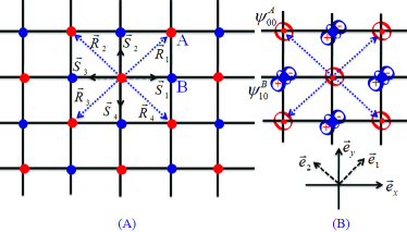
Figure 1: (Color online) (a) Fermions trapped in a 2D anisotropic square optical lattice. Due to the different on-site trapping frequencies, the square lattice is divided into two sublattices $A$ and $B$; (b) The local orbitals are in the $\vec{e}_{1}$ and $\vec{e}_{2}$ directions.

To break TR symmetry, we introduce a periodic adiabatic gauge potential in the simple form $\mathbb{A}(\mathbb{r})=\hbar A_{0}\sin(k_{0}(y-x))\vec{e}_{y}$ with $A_{0}$ a constant, which can be generated by coupling atoms to two opposite-travelling standing-wave laser beams with Rabi-frequencies $\Omega_{1}=\Omega_{0}\sin\bigr{(}k_{0}(y-x)/2+\pi/4\bigr{)}e^{-iA_{0}y},\Omega_{2}=\Omega_{0}\cos\bigr{(}k_{0}(y-x)/2+\pi/4\bigr{)}e^{iA_{0}y}$ atomgauge4 ; atomgauge6 ; experiment1 . Note the gauge field can lead to an additional contribution $|\mathbb{A}|^{2}/2m$ without the square lattice symmetry honeycomb , which, however, will not distort the present square lattice. This is because, first of all, the term $|\mathbb{A}|^{2}/2m$ is zero at all square lattice sites; secondly, the contributed potential of this term is along the $\vec{e}_{2}$ direction and leads to the same correction to $\omega_{2}^{A,B}$. Therefore we still have $\omega_{2}^{A}=\omega_{2}^{B}$ and the properties of $\psi_{a,b}$ are unchanged. This is a key difference from the situation in honeycomb lattice system, where a gauge potential with hexagonal symmetry is required to avoid the distortion of original honeycomb lattice zhu1 ; honeycomb . The simple form of gauge potential indicates here a feasible scheme in the experimental realization.

The periodic gauge potential gives rise to a Peierls phase for the hopping coefficients obtained by $\exp(i\phi^{\mathbb{r}_{i}}_{\mathbb{L}})=\exp(i\int_{\mathbb{r}_{i}}^{\mathbb{r}_{i}+\mathbb{L}}\mathbb{A}\cdot d\mathbb{r}/\hbar)$, where the integral is along the hopping path from the site $\mathbb{r}_{i}$ to site $\mathbb{r}_{i}+\mathbb{L}$. Taking into account the hopping between both the nearest and second-nearest neighbor sites, we obtain the Hamiltonian in the tight-binding form: $H=H_{1}+H_{2}+H_{z}$, with $H_{z}=M\sum_{\mathbb{r}_{i}}[C_{b}^{{\dagger}}(\mathbb{r}_{i})C_{b}(\mathbb{r}_{i})-C_{a}^{{\dagger}}(\mathbb{r}_{i})C_{a}(\mathbb{r}_{i})]$, and

$$H_{1} = -\bigr{[}\sum_{\mathbb{r}_{i}}\sum_{j=1,2}t_{ab}e^{i\phi^{\mathbb{r}_{i}}_{\mathbb{S}_{j}}}\hat{C}_{a}^{{\dagger}}(\mathbb{r}_{i})\hat{C}_{b}(\mathbb{r}_{i}+\mathbb{S}_{j})+h.c.\bigr{]}$$

$$+\bigr{[}\sum_{\mathbb{r}_{i}}\sum_{j=3,4}t_{ab}e^{i\phi^{\mathbb{r}_{i}}_{\mathbb{S}_{j}}}\hat{C}_{a}^{{\dagger}}(\mathbb{r}_{i})\hat{C}_{b}(\mathbb{r}_{i}+\mathbb{S}_{j})+h.c.\bigr{]},$$

$$H_{2} = -\sum_{\mathbb{r}_{i}}\sum_{\mu=a,b}\biggr{[}\sum_{j=1,3}t_{\mu 1}e^{i\phi^{\mathbb{r}_{i}}_{\mathbb{R}_{j}}}\hat{C}_{\mu}^{{\dagger}}(\mathbb{r}_{i})\hat{C}_{\mu}(\mathbb{r}_{i}+\mathbb{R}_{j})$$ (2)

$$+\sum_{j=2,4}t_{\mu 2}e^{(i\phi^{\mathbb{r}_{i}}_{\mathbb{R}_{j}}}\hat{C}_{\mu}^{{\dagger}}(\mathbb{r}_{i})\hat{C}_{\mu}(\mathbb{r}_{i}+\mathbb{R}_{j})\biggr{]},$$

where $\hat{C}_{\mu}(\mathbb{r}_{i})$ is the annihilation operator on site $\mathbb{r}_{i}$ in sublattices $A$ (for $\mu=a$) and $B$ (for $\mu=b$), the vectors $\mathbb{S}_{1}(-\mathbb{S}_{3})=(a,0),\mathbb{S}_{2}(-\mathbb{S}_{4})=(0,a),\mathbb{R}_{1}(-\mathbb{R}_{3})=(a,a)$ and $\mathbb{R}_{2}(-\mathbb{R}_{4})=(-a,a)$, with $a=\pi/k_{0}$ the lattice constant. It is easy to check that the Peierls phase $\phi_{R_{j}}^{\mathbb{r}_{i}}=\phi_{S_{1,3}}^{\mathbb{r}_{i}}=0$, while $\phi_{S_{2,4}}^{\mathbb{r}_{i}}=\phi_{0}$ (or $\phi_{S_{2,4}}^{\mathbb{r}_{i}}=-\phi_{0}$) with $\phi_{0}=\sqrt{2}A_{0}/k_{0}$ when the $\mathbb{r}_{i}$ site belongs to sublattice $A$ (or sublattice $B$). From the symmetry of the wave functions $\psi_{a,b}$ we know the hopping coefficients satisfy $t_{a1},t_{a2},t_{b2},t_{ab}>0;t_{b1}<0$, $t_{a1}\neq t_{a2}$ and $t_{b1}\neq t_{b2}$ (Fig. 1(b)). Besides, since the hopping constants decay exponentially with distance, $t_{ab}$ is typically several times bigger in magnitude than $t_{aj}$ and $t_{bj}$ $(j=1,2)$. Nevertheless, such differences will not affect the topological phase transition. Finally, noting $\psi_{a,b}$ have the same spatial distribution in the $\vec{e}_{2}$ direction, we can expect that $t_{a2}\approx t_{b2}$ or $|t_{a2}-t_{b2}|\ll t_{a1}-t_{b1}$.

It is convenient to transform the tight-binding Hamiltonian into momentum space, say, let $\hat{C}_{a,b}(\mathbb{r}_{j})=\frac{1}{\sqrt{N}}\sum_{\mathbb{k}}e^{i\mathbb{k}\cdot\mathbb{r}_{j}}\hat{C}_{a,b}(\mathbb{k})$ and we obtain Hamiltonian in the matrix form $H=\sum_{\mathbb{k}}\hat{\mathcal{C}}^{{\dagger}}(\mathbb{k})\mathcal{H}(\mathbb{k})\hat{\mathcal{C}}(\mathbb{k})$ with $\hat{\mathcal{C}}(\mathbb{k})=(\hat{C}_{a}(\mathbb{k}),\hat{C}_{b}(\mathbb{k}))^{T}$ and (neglecting the constant terms)

$$\mathcal{H}(\mathbb{k})=\lambda_{x}(\mathbb{k})\sigma_{x}+\lambda_{y}(\mathbb{k})\sigma_{y}+\lambda_{z}(\mathbb{k})\sigma_{z}.$$ (3)

Here $\lambda_{x}=2t_{ab}\sin\phi_{0}\sin(k_{y}a)$, $\lambda_{y}=2t_{ab}(\sin(k_{x}a)+\cos\phi_{0}\sin(k_{y}a))$ and $\lambda_{z}=-M-\Delta_{0}\cos(k_{x}a)\cos(k_{y}a)-2\tilde{t}_{1}\sin(k_{x}a)\sin(k_{y}a)$ with $\tilde{t}_{1}=(t_{a1}-t_{b1}+t_{b2}-t_{a2})/2,\Delta_{0}=t_{a1}-t_{b1}+t_{a2}-t_{b2}$. As long as $\phi_{0}\neq n\pi$, the TR symmetry of the system is broken. This Hamiltonian leads to two energy bands with the spectra given by ${\cal E}_{\pm}=\pm\sqrt{\sum_{i}\lambda_{i}^{2}(\mathbb{k})}$. One can check when $\phi_{0}\neq n\pi$, the band gap is opened if at the two independent Dirac points $\lambda_{z}(\mathbb{K}_{c})\neq 0$, with $\mathbb{K}_{C}=(0,0),(0,\pi)$. Therefore when $M\neq\pm\Delta_{0}$ the system is gapped in the bulk.

When the Fermi energy is inside the band gap, the longitudinal conductivity is zero. The anomalous Hall conductivity (AHC) can be calculated by

$$\sigma_{xy}^{H}=C_{1}/\hbar,$$ (4)

where $C_{1}=(4\pi)^{-1}\int_{FBZ}dk_{x}dk_{y}\mathbb{n}\cdot\partial_{k_{x}}\mathbb{n}\times\partial_{k_{y}}\mathbb{n}$ with $\mathbb{n}(\mathbb{k})=(\lambda_{x},\lambda_{y},\lambda_{z})/|\vec{\lambda}(\mathbb{k})|$, is the first Chern number, a quantized topological invariant defined on the first Brillouin zone (FBZ). Actually one can construct a mapping degree between FBZ torus and spherical surface $S^{2}$, $F:S^{1}\times S^{1}\mapsto S^{2}$, which gives the Chern number $C_{1}=m\in\mathbb{Z}$, with $m$ the times the mapping covers the $S^{2}$ surface. By a straightforward calculation we can show in the case $-\Delta_{0}<M<\Delta_{0}$ and thus the effective masses of the Dirac Hamiltonian around two independent Dirac points are opposite in the sign, the Chern number $C_{1}=+1$ when $0<\phi_{0}<\pi$ and $C_{1}=+1$ when $-\pi<\phi_{0}<0$. In all other cases we have $C_{1}=0$. The quantized AHC can support topological stable gapless edge states on the boundaries of the system. To study the edge modes, we consider a hard-wall boundary hardwall along $x$ axis at $x=0$ and $x=L$. The momentum $k_{x}$ is no longer a good quantum number, and we shall transform the terms with $k_{x}$ in the Hamiltonian back to position space. For convenience we envisage first the case $\phi_{0}=\pi/2$ and obtain that ($H=\sum_{k_{y},x_{i}}\mathcal{H}(k_{y},x_{i})$)

$$H = \sum_{k_{y},x_{i}}\bigr{[}\mathcal{M}\hat{C}_{k_{y},x_{i}}^{\dagger}\hat{C}_{k_{y},x_{i}}+\mathcal{A}\hat{C}_{k_{y},x_{i}}^{\dagger}\hat{C}_{k_{y},x_{i}+1}$$ (5)

$$+\mathcal{A}^{\dagger}\hat{C}_{k_{y},x_{i}+1}^{\dagger}\hat{C}_{k_{y},x_{i}}\bigr{]},$$

where

$$\mathcal{M}=2t_{ab}\sin k_{y}a\sigma_{x}-M\sigma_{z},$$ (6)

and

$$\mathcal{A} = -it_{ab}\sigma_{y}-\sum_{j=1,2}\frac{t_{aj}-t_{bj}}{2}\cos k_{y}a\sigma_{z}$$ (7)

$$+\frac{i}{2}(t_{a1}-t_{b1}+t_{b2}-t_{b1})\sin k_{y}a\sigma_{z}.$$

Note the edge modes are generally exponentially localized on the boundary edge1 . Denoting by $\Psi^{+}(k_{y},x_{i})$ and $\Psi^{-}(k_{y},x_{i})$ the edge states on the boundaries $x=0$ and $x=L$, respectively, one can verify that they take the following form

$$\Psi^{\pm}(k_{y},x_{i})=\frac{u_{k_{y}}(y)}{\sqrt{{\cal N}_{\pm}}}\bigr{[}(\xi^{(\pm)}_{1})^{x_{i}/a}-(\xi^{(\pm)}_{2})^{x_{i}/a}\bigr{]}\psi^{\pm},$$ (8)

where the complex variables $\xi_{1,2}^{\pm}$ are obtained by $\xi^{-}_{1,2}=\bigr{[}M\pm\sqrt{M^{2}+4(t_{ab}-i\tilde{t}_{1}\sin k_{y}a)^{2}-\Delta_{0}^{2}\cos^{2}k_{y}a}\bigr{]}\bigr{(}2t_{ab}-2\tilde{t}_{2}\cos k_{y}a-i2\tilde{t}_{1}\sin k_{y}a)\bigr{)}^{-1}$ and $\xi^{+}_{1,2}=1/\xi^{-}_{1,2}$, the spinor $\psi^{\pm}$ satisfies $\sigma_{x}\psi^{\pm}=\pm\psi^{\pm}$, $u_{k_{y}}(y)$ is the Bloch wave function along $y$ axis and ${\cal N}_{\pm}$ the normalization factor. The chirality of the edge modes can be found from their spectra ${\cal E}^{\pm}_{k_{y}}=\pm 2t_{ab}\sin k_{y}a$, respectively associated with group velocities $v_{F}\approx\pm 2at_{ab}/\hbar$ around Dirac point. Besides, the exponential decay of the edge states on boundaries requires that $|\xi^{+}_{1,2}|<1$ and $\xi^{-}_{1,2}>1$ edge1 . At the Dirac point $k_{y}=0$, one can check such inequalities lead to $-\Delta_{0}<M<\Delta_{0}$, which is consistent with the condition for nonzero Chern numbers obtained before. The Fig. 2 depicts the energy spectra in different situations.

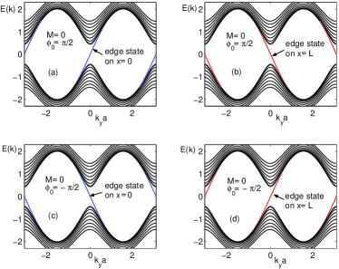
Figure 2: (Color online) Gapped bulk states (black lines) and gapless edge states (blue and red lines) on the boundaries $x=0$ ((a)(c)) and $x=L$ ((b)(d)). Parameters in (a-b) are $M=0,\phi_{0}=\pi/2$, and in (c-d) are $M=0,\phi_{0}=-\pi/2$. The chirality of edge states indicates the Chern number $C_{1}=+1$ for $\phi_{0}=\pi/2$ and $C_{1}=-1$ for $\phi_{0}=-\pi/2$.

III Detection of the topological phase transition

Next we proceed to study the detection of the edge and bulk states with light Bragg scattering, with which one can detect the topological phase transition. In the Bragg spectroscopy, we shine two lasers on the lattice system, with the wave vectors $\mathbb{k}_{1},\mathbb{k}_{2}$ and frequencies $\omega_{1,2}=k_{1,2}c$, respectively (Fig. 3(a)). Note only the momentum $k_{y}$ is still a good quantum number, we let $\mathbb{q}=\mathbb{k}_{1}-\mathbb{k}_{2}=q\hat{e}_{y}$ and denote $\omega=\omega_{1}-\omega_{2}$. The atom-light interacting Hamiltonian reads

$$H_{int}=\sum_{k_{1y},k_{2y}}\Omega e^{i\mathbb{q}\cdot\mathbb{r}}\hat{C}_{\mu}^{\dagger}(k_{y}+\mathbb{q})\hat{C}_{\nu}(k_{y})+h.c.,$$ (9)

where $\Omega$ is an effective Rabi-frequency of the two-photon process in light Bragg scattering, and the indices $\mu,\nu$ may represent the edge or bulk states. The light Bragg scattering directly measures the dynamical structure factorBragg :

$$S(\mathbb{q},\omega) = \sum_{k_{y_{1}},k_{y_{2}}}(1-f(E^{(f)}_{k_{y_{2}}}))f(E^{(i)}_{k_{y_{1}}})\times$$ (10)

$$\times |\langle\Psi_{k_{y_{2}}}^{(f)}|H_{int}|\Psi_{k_{y_{1}}}^{(i)}\rangle|^{2}\delta(\hbar\omega-E^{(f)}_{k_{y_{2}}}+E^{(i)}_{k_{y_{1}}})$$

with $|\Psi_{k_{y_{1}}}^{(i)}\rangle$ ($|\Psi_{k_{y_{2}}}^{(f)}\rangle$) initial (final) atomic state before (after) scattering and $f(E)$ the Fermi distribution function. For the topological insulating phase, e.g. when $\phi_{0}=\pi/2$ and $M=0$, since the edge states are localized on the boundaries, we may consider two basic situations for the Bragg scattering, say, first we shine the two lasers on one boundary (on $x=0$ or $x=L$) of the system; secondly we shine them on the whole lattice system including both boundaries. For the former case, only edge states on the boundary shined with lasers can be scattered. When $\omega<\Delta_{0}$, the initial edge states below Fermi energy will be scattered to edge states above Fermi energy, while for $\omega>\Delta_{0}$, part of the initial edge states can be pumped to upper band bulk states after scattering. Note that the edge state is an exponential decaying function in the $x$ direction, with decaying property dependent on the momentum $k_{y_{1}}$, while the bulk states are standing waves along $x$ axis. Therefore, the scattering process with an edge state pumped to bulk states actually includes many channels characterized by different values of $k_{x_{2}}$ of the final bulk states, and the effective Rabi-frequency for such scattering processes is generally a function of $k_{y_{1}},k_{x_{2}}$, denoted by $\tilde{\Omega}(k_{y_{1}},k_{x_{2}})$. Nevertheless, in the practical case, we require $\omega$ is slightly above $\Delta_{0}$, and only the states with momenta near zero need to be considered. In this way we can expect $\tilde{\Omega}$ does not change considerably from $\tilde{\Omega}_{0}\equiv\tilde{\Omega}(0,0)$, and can be expanded around this value. Specifically, in continuum limit one finds the exponential decay property of the edge state (localized on $x=0$) given in Eq. (8) can be approximated as $\Psi^{+}\sim e^{-q_{0}x}$ with $q_{0}=\frac{\Delta_{0}}{2at_{ab}}$, with which we obtain the effective Rabi-frequency $\tilde{\Omega}(k_{x},k_{y})\approx\tilde{\Omega}_{0}/(q_{0}^{2}+k_{x}^{2})$. Bearing these results in mind, we can verify for $|q|\geq q_{0}$, the dynamical structure takes the following general form

$$S(\mathbb{q},\omega) \approx (|q|+k_{y_{0}})\Omega^{2}\delta(\omega\mp v_{F}q)$$ (11)

$$+ \frac{\Delta_{0}\tilde{\Omega}^{2}_{0}}{2t_{ab}^{2}a^{2}}\frac{1+3\hbar\tilde{\omega}/(2q_{0}at_{ab})}{[1+\hbar\tilde{\omega}/(q_{0}at_{ab})]^{2}}\times$$

$$\times \biggr{[}\frac{\pi}{2}+\sin^{-1}\frac{\alpha^{1/2}|q-q_{0}|}{\sqrt{\hbar\tilde{\omega}}}\biggr{]}\Theta(\omega-\omega_{c}),$$

where $\tilde{\omega}=\omega-\Delta_{0}/2\hbar-2|q|at_{ab}/\hbar,\omega_{c}=(\Delta_{0}/2+2|q|at_{ab})/\hbar,\alpha=2\Delta_{0}^{-1}t_{ab}^{2}a^{2}$, and the step function $\Theta(x)=1(0)$ for $x>0$ ($x<0$). For $q<q_{0}$, the $S(\mathbb{q},\omega)$ is obtained in the same form, only with $\omega_{c}$ changed to be $\omega_{c}=(\Delta_{0}+2a^{2}t_{ab}^{2}q^{2}/\Delta_{0})/\hbar$ in Eq. (11). The first term in $S(\mathbb{q},\omega)$ is contributed by the scattering processes with edge states pumped to edge states on the boundary $x=0$ (for “$-$”) or $x=L$ (for “$+$”). The peaks at $\omega=\pm qv_{F}$ obtained by this term reflects the chirality of the edge modes (Fig. 3(b-c), the blue solid line). From the second term in $S(\mathbb{q},\omega)$ we see the scattering processes with initial edge states pumped to the upper band bulk states approximately give rise to a finite contribution (Fig. 3(b-c), the red dashed line). For the latter situation the lasers are shined on the whole lattice, the cross scattering process with edge states on one boundary scattered to edge states on another boundary will happen. We can show that the cross scattering leads to an additional contribution $\frac{\Omega^{2}}{\hbar v_{F}}\Theta(\omega\mp v_{F}q)$ to the dynamical structure (Fig. 3(c), the blue dotted line).

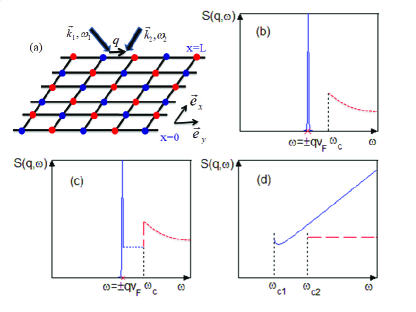
Figure 3: (Color online) Schematic of light Bragg Scattering (a) and dynamical structure for the cases that the system is in the topological phase (b-c), and in the insulating phase (d).

Finally, when $|M|\geq\Delta_{0}$, the Chern number becomes zero and in this case no edge state can survive on the boundaries. Specifically, for the case $M=-\Delta_{0}$ (and $\phi_{0}=\pi/2$), the bulk gap is closed ($\Delta=0$ at the Fermi point $\mathbb{k}=0$) and the particles can be described as massless Fermions duan , while for $M=-2\Delta_{0}$, the bulk gap is given by $\Delta=2\Delta_{0}$. We respectively obtain the dynamical structure for the two cases $S(\mathbb{q},\omega)=\frac{\pi\Omega^{2}}{16a^{2}t_{ab}^{2}}\frac{\hbar^{2}\omega^{2}-2a^{2}t_{ab}^{2}q^{2}}{\sqrt{\hbar^{2}\omega^{2}-4a^{2}t_{ab}^{2}q^{2}}}\Theta(\omega-\omega_{c_{1}})$ and $S(\mathbb{q},\omega)=\frac{\pi\Delta_{0}\Omega^{2}}{4a^{2}t_{ab}^{2}}\Theta(\omega-\omega_{c_{2}})$, with $\omega_{c_{1}}=2at_{ab}q/\hbar$ and $\omega_{c_{2}}=(2\Delta_{0}+q^{2}a^{2}t_{ab}^{2}/\Delta_{0})/\hbar$. The results are plotted with blue solid line (for $\Delta=0$) and red dashed line (for $\Delta=2\Delta_{0}$) in Fig. 3(d). Based on the results of light Bragg scattering in different situations, we clearly see the Bragg spectroscopy provides a direct way to observe the edge states and bulk states.

IV conclusion

In conclusion, we proposed a novel scheme to realize the quantum anomalous Hall effect in an anisotropic square optical lattice based on the experiment set-up of the double-well lattice at NIST. We have studied in detail the experimental detection of the edge and bulk states through light Bragg scattering, with which one can determine the topological phase transition from usual insulating phase to quantum anomalous Hall phase.

This work was supported by ONR under Grant No. ONR-N000140610122, by NSF under Grant No. DMR-0547875, and by SWAN-NRI. Jairo Sinova is a Cottrell Scholar of the Research Corporation. C.W. is supported by NSF-DMR0804775.

References

- (1) F. D. M. Haldane, Phys. Rev. Lett. 61, 2015 (1988).
- (2) K.V. Klitzing, G. Dorda, and M. Pepper, Phys. Rev. Lett. 45, 494 (1980).
- (3) R. B. Laughlin, Phys. Rev. B 23, 5632 (1981).
- (4) B. I. Halperin, Phys. Rev. B 25, 2185 (1982).
- (5) D.J. Thouless, M. Kohmoto, M.P. Nightingale, and M. den Nijs, Phys. Rev. Lett., 49, 405 (1982).
- (6) C. -X. Liu, X. -L. Qi, X. Dai, Z. Fang and S. -C. Zhang, Phys. Rev. Lett. 101, 146802 (2008).
- (7) X. -L. Qi, Y.S. Wu, and S.C. Zhang, Phys. Rev. B 74, 045125 (2006).
- (8) B.A. Bernevig, Taylor L. Hughes and S.-C. Zhang, Science, 314, 1757, (2006).
- (9) M. König et al., Science 318, 766 (2007).
- (10) L. B. Shao, S. -L. Zhu, L. Sheng, D.Y. Xing and Z. D.Wang, Phys. Rev. Lett. 101, 246810 (2008).
- (11) J. Ruseckas, G. Juzeliunas, P. Ohberg, and M. Fleischhauer, Phys. Rev. Lett. 95, 010404 (2005).
- (12) S.-L. Zhu, H. Fu, C.-J. Wu, S.-C. Zhang and L.-M. Duan, Phys. Rev. Lett. 97, 240401 (2006).
- (13) X. -J. Liu, Mario F. Borunda, Xin Liu, and Jairo Sinova, Phys. Rev. Lett. 102, 046402 (2009).
- (14) Y. -J. Lin, R. L. Compton, A. R. Perry, W. D. Phillips, J. V. Porto, and I. B. Spielman, Phys. Rev. Lett. 102, 130401 (2009).
- (15) J. -M. Hou, Wen-Xing Yang, and Xiong-Jun Liu, Phys. Rev. A 79, 043621 (2009).
- (16) Congjun Wu, Phys. Rev. Lett. 101, 186807 (2008).
- (17) N. Gemelke, Ph.D. thesis, Stanford University, 2007.
- (18) J. Sebby-Strabley et al., Phys. Rev. A 73, 033605 (2006); Phys. Rev. Lett. 98, 200405 (2007).
- (19) Tudor D. Stanescu et al., Phys. Rev. A 79, 053639 (2009).
- (20) I. Bloch, Jean Dalibard, Wilhelm Zwerger, Rev. Mod. Phys. 80, 885 (2008).
- (21) T. P. Meyrath, F. Schreck, J. L. Hanssen, C.-S. Chuu, and M. G. Raizen, Phys. Rev. A 71, 041604(R) (2005).
- (22) M. König, Hartmut Buhmann, Laurens W. Molenkamp, Taylor Hughes, Chao-Xing Liu, Xiao-Liang Qi1, and Shou-Cheng Zhang J. Phys. Soc. Jpn. 77, 031007 (2008).
- (23) D.M. Stamper-Kurn et al., Phys. Rev. Lett. 83, 2876 (1999).
- (24) S. -L. Zhu, Baigeng Wang, and L.-M. Duan, Phys. Rev. Lett. 98, 260402 (2007).