Asymptotic behaviour of convex and column-convex lattice polygons with fixed area and varying perimeter

Abstract

We study the inflated phase of two dimensional lattice polygons, both convex and column-convex, with fixed area $A$ and variable perimeter, when a weight $\mu^{t}\exp[-Jb]$ is associated to a polygon with perimeter $t$ and $b$ bends. The mean perimeter is calculated as a function of the fugacity $\mu$ and the bending rigidity $J$. In the limit $\mu\rightarrow 0$, the mean perimeter has the asymptotic behaviour $\langle t\rangle/4\sqrt{A}\simeq 1-K(J)/(\ln\mu)^{2}+\mathcal{O}(\mu/\ln\mu)$. The constant $K(J)$ is found to be the same for both types of polygons, suggesting that self-avoiding polygons should also exhibit the same asymptotic behaviour.

Keywords: vesicles and membranes, loop models and polymers, exact results, series expansions

1 Introduction

The enumeration of lattice polygons weighted by area and perimeter arises in many physical systems, including vesicles [1, 2], cell membranes [3], emulsions [4], polymers [5] and percolation clusters [6]. A central quantity of interest is the generating function

$$G(P,\mu,J)=\sum_{A,t,b}C(A,t,b)e^{PA}\mu^{t}e^{-Jb},$$ (1)

where $C(A,t,b)$ is the number of self-avoiding polygons of area $A$, perimeter $t$ and with $b$ bends. This is weighted by a pressure $P$ (conjugate to the area), a fugacity $\mu$ (conjugate to the perimeter) and a bending rigidity $J$ (conjugate to the number of bends).

Exact solutions exist for $G(P,\mu,0)$ when $C(A,t,b)$ is restricted to convex polygons [7, 8, 9] or to column-convex polygons [10]. However, a general solution for self-avoiding polygons is unavailable and even the exact solutions for these restricted polygons are complex enough that extracting the asymptotics is non-trivial. The properties of self-avoiding polygons can be studied by enumerating the number of configurations that correspond to a given area and perimeter. Exact enumeration results for self-avoiding polygons exist for values of the area $A$ up to $A=50$ and for all $t$ for these values of $A$ [11, 12]. The scaling function describing the scaling behaviour near the tricritical point $\lambda=0$ and $\mu=\kappa^{-1}$, where $\kappa$ is the growth constant for self-avoiding polygons, is also known exactly [13, 14, 15]. A survey of different kinds of lattice polygons and a review of related results can be found in Refs. [16, 17].

In an earlier paper [18], we determined the mean area of inflated convex and column-convex polygons of fixed perimeter as a function of the pressure and bending rigidity. This case relates to the problem of two-dimensional vesicles, or equivalently, pressurised ring polymers [1, 19, 20, 21, 22] on a square lattice. We showed that in the limit of large pressure, the expression for the average area was the same for convex and column-convex polygons. We also verified numerically that the same result held for the case of self-avoiding polygons.

In this paper, we consider the related problem of determining the mean perimeter of a polygon of fixed area. We calculate the mean perimeter for convex [see Eq. (29)] and column-convex [see Eqs. (3.2,48)] polygons exactly. In the limit $\mu\rightarrow 0$, corresponding to inflated polygons, we show that for both convex and column-convex polygons, the perimeter is given by

$$\langle t\rangle=4\sqrt{A}\left[1-\frac{1}{2(\ln\mu)^{2}}\int_{1-\alpha}^{1}dx\frac{\ln(1-x)}{x}\right]+\mathcal{O}(\mu/\ln\mu),$$ (2)

where $\alpha=e^{-2J}$. Since this result is the same for both convex and row-convex polygons, we argue that this result should therefore also extend to the self-avoiding case.

In Sec. 2, we outline the calculation scheme for determining the mean perimeter. The results for convex polygons and column-convex polygons are presented in Sec. 3.1 and Sec. 3.2 respectively. In Sec. 4, we generalise these results to the case of self avoiding polygons and compare the analytical results with results from exact enumeration studies.

2 Outline of the calculation

Convex polygons are those polygons that have exactly $0$ or $2$ intersections with any vertical or horizontal line drawn through the midpoints of the edges of the lattice (Fig. 1 (a)). Column-convex polygons are those polygons that have exactly $0$ or $2$ intersections with any vertical line drawn through the midpoints of the edges of the lattice. There is, however, no such restriction in the horizontal direction (Fig. 1 (b)). Self avoiding polygons are polygons that have no restrictions on overhangs.

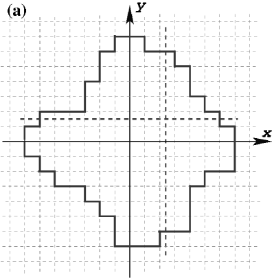
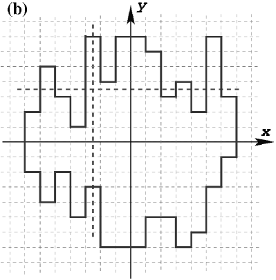
Figure 1: (a) Schematic diagram of a convex polygon. Any vertical or horizontal line (thick dashed lines) intersects the convex polygon at either $0$ or $2$ points. (b) Schematic diagram of a column-convex polygon. Any vertical line (thick dashed lines) intersects the convex polygon at either $0$ or $2$ points.

The shapes of convex and row-convex polygons are obtained by minimising the free energy at fixed area, generalising the calculation presented in Ref. [18]. The equilibrium shape of convex polygons is invariant under rotations by $\pi/2$. Let the shape in the first quadrant be represented by a curve $y_{1}(x)$ with endpoints at $(a\sqrt{A},0)$ and $(0,a\sqrt{A})$, where $A$ is the area of the polygon (see Fig. 2(a)). In the case of column-convex polygons, the equilibrium shape is invariant under reflection about the x-axis. Let $y_{2}(x)$ be the shape of the column-convex polygon in the upper half plane with endpoints at $(-b\sqrt{A},0)$ and $(b\sqrt{A},0)$ (see Fig. 2(b)). The free energy functionals for these shapes can be written as

$$\mathcal{L}_{1} = \int_{0}^{a\sqrt{A}}\!\!\!\!dx\sigma_{1}(y_{1}^{\prime})\sqrt{1+y_{1}^{\prime 2}}-\frac{\lambda_{1}}{\sqrt{A}}\int_{0}^{a\sqrt{A}}\!\!\!\!y_{1}dx,$$ (3)

for convex polygons and

$$\mathcal{L}_{2} = \int_{-b\sqrt{A}}^{b\sqrt{A}}\!\!\!\!dx\sigma_{2}(y_{2}^{\prime})\sqrt{1+y_{2}^{\prime 2}}-\frac{\lambda_{2}}{\sqrt{A}}\int_{-b\sqrt{A}}^{b\sqrt{A}}\!\!\!\!y_{2}dx,$$ (4)

for column-convex polygons. The subscripts $1$ ($2$) denote convex (column-convex) polygons, $\sigma$ is the free energy per unit length associated with a slope $y^{\prime}$ and $\lambda$’s are Lagrange multipliers. The Lagrange multipliers have been scaled by $\sqrt{A}$ so that they become intensive quantities.

Figure 2: A schematic diagram of the equilibrium shape of (a) convex polygon: the shapes in the other quadrants are obtained by symmetry. (b) column-convex polygons: the shape in the lower half plane is obtained by reflection.

The angle dependent surface tension $\sigma$ was computed in [18] using simple combinatorial arguments. For convex polygons $\sigma_{1}$ is given by

$$\sigma_{1}(y^{\prime})\sqrt{1+y^{\prime 2}}=-f_{1}(\omega^{*})-2\ln(\mu),$$ (5)

where

$$f_{1}(\omega)=y^{\prime}\ln(\omega)+\ln[1-(1-\alpha)\omega]-\ln(1-\omega),$$ (6)

and $\omega^{*}$ satisfies

$$\left.\frac{df_{1}}{d\omega}\right|_{\omega^{*}}=0,$$ (7)

and $\alpha=e^{-2J}$.

For column-convex polygons, the surface tension $\sigma_{2}$ is of the form [18]

$$\sigma_{2}(y^{\prime})\sqrt{1+y^{\prime 2}}=iB_{0}y^{\prime}-\ln\mu-\ln f_{2}(\mu,\alpha,B_{0}),$$ (8)

where

$$f_{2}(\mu,\alpha,B)=\frac{1+(1-2\alpha)\mu^{2}+\mu(\alpha-1)(e^{iB}+e^{-iB})}{(1-\mu e^{iB})(1-\mu e^{-iB})}.$$ (9)

and $B_{0}$ satisfies the equation,

$$\frac{d}{dB_{0}}\ln f_{2}(\mu,\alpha,B_{0})=iy^{\prime}.$$ (10)

The equilibrium shape is obtained from Eqs. (3) and (4) by solving the Euler Lagrange equation [23],

$$\frac{d}{dx}\frac{d}{dy^{\prime}}\left[\sigma_{1,2}(y^{\prime})\sqrt{1+y^{\prime 2}}\right]=-\frac{\lambda_{1,2}}{\sqrt{A}}.$$ (11)

Using the above expressions for the surface tension $\sigma$, the equilibrium shapes of convex and column-convex polygons were computed exactly by solving the Euler Lagrange equations. We reproduce the final results, which will be the starting point of the calculations presented in the next section. For convex polygons, the equilibrium shape is given by

$$y_{1}=\frac{\sqrt{A}}{\lambda_{1}}\ln\left[\frac{1-c_{1}e^{\lambda_{1}x/\sqrt{A}}}{\left[1-c_{1}(1-\alpha)e^{\lambda_{1}x/\sqrt{A}}\right]c_{1}}\right],$$ (12)

with the constant $c_{1}$ being given by,

$$c_{1}=\frac{(1+e^{\lambda_{1}a})-\sqrt{(1+e^{\lambda_{1}a})^{2}-4e^{\lambda_{1}a}(1-\alpha)}}{2(1-\alpha)e^{\lambda_{1}a}}.$$ (13)

The equilibrium shape for column convex polygons is given by [18]

$$y_{2}(x)=-\frac{\sqrt{A}}{\lambda_{2}}\times$$

$$\!\!\ln\left[\frac{(1-\mu e^{\lambda_{2}x/\sqrt{A}})(1-\mu e^{-\lambda_{2}x/\sqrt{A}})e^{-c_{2}}}{1+(1-2\alpha)\mu^{2}+\mu(\alpha-1)(e^{\lambda_{2}x/\sqrt{A}}+e^{-\lambda_{2}x/\sqrt{A}})}\right],$$

where the constant $c_{2}$ is given by

$$c_{2}=\ln\frac{(1-\mu g_{2})(1-\mu g_{2}^{-1})}{1+(1-2\alpha)\mu^{2}+\mu(\alpha-1)(g_{2}+g_{2}^{-1})},$$ (15)

where, $g_{2}=\exp(\lambda_{2}b)$. The constants $a$ and $b$ (see Fig. 2) are chosen so that the free energy is minimised.

3 Results

Starting from the equilibrium shapes [Eqs. (12) and (2)] described in Sec. 2, we now calculate the mean perimeter of convex and column-convex polygons of fixed area $A$.

3.1 Convex polygons

The Lagrange multiplier $\lambda_{1}$ is determined by the constraint that the area under the curve is $A/4$:

$$\int_{0}^{a\sqrt{A}}y_{1}dx=\frac{A}{4}.$$ (16)

Substituting for the form of the equilibrium curve as given by Eq. (12), we obtain,

$$\frac{\lambda_{1}^{2}}{4}=\int_{0}^{\ln g_{1}}dz\ln\left[\frac{1-c_{1}e^{z}}{c_{1}[1-c_{1}(1-\alpha)e^{z}]}\right],$$ (17)

where $g_{1}=\exp(\lambda_{1}a)$.

The free energy of the equilibrium shape is obtained by substituting the expressions for the equilibrium curve Eq. (12) and the surface tension Eq. (5), into Eq. (3). Simplifying, we obtain

$$\mathcal{L}_{1}=\frac{\lambda_{1}\sqrt{A}}{2}+2a\sqrt{A}\ln c_{1}-2\ln\mu~{}a\sqrt{A}.$$ (18)

The parameter $a$ is chosen to be that value that minimises the above expression for the free energy, i.e. $a$ satisfies $\partial{\mathcal{L}_{1}}/\partial{a}=0$. This gives,

$$\frac{1}{2}\frac{d\lambda_{1}}{da}+2\ln c_{1}+\frac{2a}{c_{1}}\frac{dc_{1}}{da}-2\ln\mu=0.$$ (19)

To calculate the first term, we differentiate Eq. (17) with respect to $a$ to obtain

$$\frac{\lambda_{1}}{2}\frac{d\lambda_{1}}{da} = \frac{1}{c_{1}}\frac{dc_{1}}{da}\ln\!\!\left[\frac{(1-c_{1}g_{1})(1-c_{1})^{-1}g_{1}^{-1}}{[1-c_{1}(1-\alpha)g_{1}][1-c_{1}(1-\alpha)]}\right],$$ (20)

where the constant $c_{1}$ can be expressed in terms of $g_{1}$ as

$$c_{1}=\frac{1+g_{1}-\sqrt{(1+g_{1})^{2}-4(1-\alpha)g_{1}}}{2(1-\alpha)g_{1}}.$$ (21)

Substituting for $d\lambda_{1}/da$ from Eq. (20) and using Eq. (21) and simplifying, we obtain the solution

$$c_{1}=\mu.$$ (22)

The expression for $g_{1}$ for this value of $c_{1}$ is obtained by replacing $c_{1}$ with $\mu$ in Eq. (21) :

$$g_{1}=\frac{1-\mu}{\mu+\mu^{2}(\alpha-1)}.$$ (23)

Knowing $g_{1}$, the parameter $a$ can easily be obtained as

$$a=\frac{1}{\lambda_{1}}\ln g_{1}=\frac{1}{\lambda_{1}}\ln\big{[}\frac{1}{\mu(1+\mu(\alpha-1))}\big{]}.$$ (24)

The value of the mean perimeter is equal to

$$\langle t\rangle=8a\sqrt{A},$$ (25)

where the factor $8$ accounts for all the four quadrants.

When $\mu\rightarrow 0$, the shape reduces to a square and the perimeter equals $4\sqrt{A}$. We would like to find the corrections for small values of $\mu$. For small $\mu$,

$$\ln g_{1}=-\ln\mu-\mu(\alpha-1)+O(\mu^{2}).$$ (26)

Expanding the expression Eq. (17) for $\lambda_{1}$ for small $\mu$, we obtain

$$\frac{\lambda_{1}^{2}}{4}=(\ln\mu)^{2}\big{[}1+\frac{1}{(\ln\mu)^{2}}\int_{1-\alpha}^{1}dx\frac{\ln(1-x)}{x}\big{]}+O\left(\frac{\mu}{\ln\mu}\right).$$ (27)

The parameter $a$ is then given by,

$$a = \frac{1}{\lambda_{1}}\ln g_{1}$$ (28)

$$= \frac{1}{2}-\frac{1}{4(\ln\mu)^{2}}\int_{1-\alpha}^{1}dx\frac{\ln(1-x)}{x}+O\left(\frac{\mu}{\ln\mu}\right).$$

The total perimeter $t=8a\sqrt{A}$ is then given by,

$$\frac{\langle t\rangle}{4\sqrt{A}}=1-\frac{1}{2(\ln\mu)^{2}}\int_{1-\alpha}^{1}dx\frac{\ln(1-x)}{x}+O\left(\frac{\mu}{\ln\mu}\right).$$ (29)

The results for the mean perimeter for convex polygons are shown in Fig. 3.

3.2 Column-convex polygons

In this section, we calculate the mean perimeter of column-convex polygons of area $A$ for arbitrary $\mu>0$. We start with Eqs. (4), (8), (2) and (15).

The Lagrange multiplier $\lambda_{2}$ is fixed by the constraint,

$$\int_{-b\sqrt{A}}^{b\sqrt{A}}y_{2}dx=\frac{A}{2}.$$ (30)

On simplifying, this gives,

$$\frac{\lambda_{2}^{2}}{4}=$$

$$\int_{0}^{\ln g_{2}}dz\left[\ln\frac{(1-\mu e^{z})(1-\mu e^{-z})}{1+(1-2\alpha)\mu^{2}+\mu(\alpha-1)(e^{z}+e^{-z})}-c_{2}\right],$$

where $\ln g_{2}=\lambda_{2}b$.

The total free energy of the curve with ends fixed as $(-b\sqrt{A},0)$ and $(b\sqrt{A},0)$ can be calculated by substituting the equation for the equilibrium curve [Eq. (2)] into the expression for the Lagrangian [Eq. (4)]and simplifying, thus yielding

$$\mathcal{L}_{2}=\sqrt{A}[\lambda_{2}+2b(c_{2}-\ln\mu)].$$ (32)

The parameter $b$ is fixed by the condition that the free energy should be a minimum, i.e. $d\mathcal{L}_{2}/db=0$ :

$$\frac{d\lambda_{2}}{db}+2(c_{2}-\ln\mu)+2b\frac{dc_{2}}{db}=0.$$ (33)

The first term is calculated by differentiating Eq. (32) with respect to b,

$$\frac{1}{2}\frac{d\lambda_{2}}{db}=-b\frac{dg}{db}\frac{dc_{2}}{dg}.$$ (34)

Substituting Eq. (34) into Eq. (33) and simplifying, we obtain

$$c_{2}=\ln\mu.$$ (35)

This immediately allows the solution of $g_{2}$ by substituting for $c_{2}$ in Eq. 15,

$$g_{2} = \frac{1-\mu+\mu^{2}+\mu^{3}(2\alpha-1)}{2\mu[1+(\alpha-1)\mu]}$$

$$+ \frac{\sqrt{(1-\mu^{2})(1-2\mu+2(1-2\alpha)\mu^{3}-(1-2\alpha)^{2}\mu^{4})}}{2\mu[1+(\alpha-1)\mu]}.$$

The average perimeter is related to the chemical potential $\mu$ by the relation,

$$\langle t\rangle=-2\mu\frac{\partial{\mathcal{L}_{2}}}{\partial{\mu}},$$ (37)

where the factor of two accounts for the equilibrium shape in the lower half plane also. Substituting for the free energy, this implies,

$$\frac{\langle t\rangle}{4\sqrt{A}}=-\frac{\mu}{2}\frac{\partial{\lambda_{2}}}{\partial{\mu}}.$$ (38)

Now, using Eq. 3.2 for $\lambda_{2}$ and simplifying, we obtain,

$$\frac{\langle t\rangle}{4\sqrt{A}} = -\frac{1}{\lambda_{2}}\ln\left[\frac{1-\mu g_{2}}{g_{2}(g_{2}-\mu)}\right]$$

$$- \left(\frac{1+\mu^{2}(2\alpha-1)}{\lambda_{2}\sqrt{k_{1}^{2}-k_{2}^{2}}}\times\right.$$

$$\left.\ln\left[\frac{(k_{1}+k_{2})(g_{2}+1)+\sqrt{k_{1}^{2}-k_{2}^{2}}(g_{2}-1)}{(k_{1}+k_{2})(g_{2}+1)-\sqrt{k_{1}^{2}-k_{2}^{2}}(g_{2}-1)}\right]\right),$$

where $k_{1}$ and $k_{2}$ are given by,

$$k_{1} = 1+(1-2\alpha)\mu^{2},$$ (40)

$$k_{2} = 2\mu(\alpha-1).$$ (41)

We would now like to determine the small $\mu$ behaviour of the mean perimeter. As in the case of the convex polygon, Eq. (3.2) reduces to

$$\ln g_{2}=-\ln\mu-\alpha\mu+\mathcal{O}(\mu^{2}).$$ (42)

In this limit, we can expand the right hand side of Eq. (3.2) as

$$\frac{t}{4\sqrt{A}}=\frac{1}{\lambda_{2}}[-2\ln\mu-\alpha\mu+\mathcal{O}(\mu^{2}\ln\mu)].$$ (43)

Finally, we require the expansion of $\lambda_{2}$ in terms of $\mu$ and $\ln\mu$. The equation for the Lagrange multiplier $\lambda_{2}$, Eq. 3.2, can be expanded as,

$$\frac{\lambda_{2}^{2}}{4} = \int_{\mu}^{1-\alpha\mu}dx\frac{\ln(1-x)}{x}+\int_{\mu^{2}}^{\mu}dx\frac{\ln(1-x)}{x}-\ln g_{2}\ln\mu$$

$$- \int_{0}^{\ln g_{2}}dz\ln\left[1+(1-2\alpha)\mu^{2}+\mu(\alpha-1)(e^{z}+e^{-z})\right],$$

where we have used the identities,

$$\int_{0}^{\ln g_{2}}dz\ln(1-\mu e^{z}) = \int_{\mu}^{1-\alpha\mu}dx\frac{\ln(1-x)}{x},$$ (45)

$$\int_{0}^{\ln g_{2}}dz\ln(1-\mu e^{-z}) = \int_{\mu^{2}}^{\mu}dx\frac{\ln(1-x)}{x}.$$ (46)

On further simplification, this yields, in the limit $\mu\rightarrow 0$,

$$\lambda_{2}=2\ln\mu\left[1+\frac{\int_{1-\alpha}^{1}dx\ln(1-x)/x}{2(\ln\mu)^{2}}\right].$$ (47)

Substituting for $\lambda_{2}$ in Eq. 43, we obtain the average perimeter for column-convex polygons as,

$$\frac{\langle t\rangle}{4\sqrt{A}}\simeq 1-\frac{1}{2(\ln\mu)^{2}}\int_{1-\alpha}^{1}dx\frac{\ln(1-x)}{x}+\mathcal{O}(\mu/\ln\mu).$$ (48)

The column-convex polygon results, both for the general case and in the small $\mu$ approximation, are shown in Fig. 3.

4 Self Avoiding Polygons

In Sec. 3, we calculated, as a function of the fugacity $\mu$ and bending rigidity $J$, the mean perimeter of convex and column-convex polygons of fixed area $A$. For small $\mu$, the expression for the perimeter takes the form

$$\frac{\langle t\rangle}{4\sqrt{A}}\simeq 1-\frac{1}{2(\ln\mu)^{2}}\int_{1-\alpha}^{1}dx\frac{\ln(1-x)}{x}+\mathcal{O}(\mu/\ln\mu),$$ (49)

for both convex and column-convex polygons. This is similar to the case of polygons with fixed perimeter, where the asymptotic expressions for area match up to the second term as well [18]. Introducing overhangs in one direction to convert convex polygons to column-convex polygons does not affect the second term in the expansion Eq. (49). It is therefore plausible that introducing overhangs in the vertical direction also does not affect the above expression, and hence that the mean perimeter of self-avoiding polygons should also be described by the expression given in Eq. (49), for small $\mu$.

Figure 3: The mean perimeter for convex and column-convex polygons are compared with the small $\mu$ expansion result and data from exact enumeration of self avoiding polygons of area $A$ up to $A=49$.

In order to test this conjecture numerically, we used exact enumeration data for polygons on the square lattice for the case $J=0$. For self-avoiding polygons, exact enumerations are available for areas up to $A=49$ [12]. The resulting plot for the average perimeter is shown in Fig. 3. Unfortunately, with the data currently available it is not possible to extrapolate to infinite $N$, preventing an unambiguous test of this conjecture. Also, we know of no simple Monte Carlo algorithm that preserves area while varying perimeter, by which one could access higher areas.

5 Summary and conclusions

We now summarise the basic results of this paper. We have studied the variation of the perimeter, as a function of the chemical potential $\mu$ and bending rigidity $J$, for fixed area, for both convex and column-convex polygons. In each of these cases, we have calculated the perimeter exactly. The asymptotic behaviour in the limit $\mu\rightarrow 0$ coincides for both classes of polygons. We therefore conjecture that overhangs are not important in the inflated regime, and hence that self avoiding polygons should have the same asymptotic behaviour. It is important to obtain a numerical confirmation or rigorous proof of this conjecture.

References

References

• [1] Leibler S, Singh R P and Fisher M E 1987 Phys. Rev. Lett. 59 1989
• [2] Fisher M E, Guttmann A J and Whittington S G 1991 J. Phys. A 24 3095
• [3] Satyanarayana S V M and Baumgaertner A 2004 J. Chem. Phys. 121 4255
• [4] van Faassen E 1998 Physica A 255 251
• [5] Privman V and Svrakic N M 1989 Directed Models of Polymers, Interfaces, and Clusters: Scaling and Finite-Size Properties (Springer-Verlag)
• [6] Rajesh R and Dhar D 2005 Phys. Rev. E 71 016130
• [7] Lin K Y 1991 J. Phys. A. 24 2411
• [8] Bousquet-Melou M 1992 J. Phys. A 25 1925
• [9] Bousquet-Melou M 1992 J. Phys. A. 25 1935
• [10] Brak R and Guttmann A J 1990 J. Phys. A 23 4581
• [11] Jensen I 2003 J. Phys. A 36 5731
• [12] Jensen I, Number of sap of given perimeter and any area, available at the website http://www.ms.unimelb.edu.au/Β iwan/polygons/series/sqsap_area_perim.ser
• [13] Richard C, Guttmann A J and Jensen I 2001 J. Phys. A 34 L495
• [14] Cardy J 2001 J. Phys. A 34 L665
• [15] Richard C 2002 J. Stat. Phys. 108 459
• [16] Bousquet-Melou M 1996 Discrete Math. 154 1
• [17] van Rensburg E J J 2000 The Statistical Mechanics of Interacting Walks, Polygons, Animals and Vesicles (Oxford University Press)
• [18] Mitra M K, Menon G I and Rajesh R 2008 J. Stat. Phys. 131 393
• [19] Rudnick J and Gaspari G 1991 Science 252 422
• [20] Gaspari G, Rudnick J and Beldjenna A 1993 J. Phys. A 26 1
• [21] Haleva E and Diamant H 2006 Eur. Phys. J. E 19 461
• [22] Mitra M K, Menon G I and Rajesh R 2008 Phys. Rev E 77 041802
• [23] Rottman C and Wortis M 1984 Phys. Rep. 103 59