Lattice Boltzmann simulations of liquid film drainage between smooth surfaces

Abstract

Exploring the hydrodynamic boundary of a surface by approaching a colloidal sphere and measuring the occurring drag force is a common experimental technique. However, numerous parameters like the wettability and surface roughness influence the result. In experiments these cannot be separated easily. For a deeper understanding of such surface effects a tool is required that predicts the influence of different surface properties. In this paper we present computer simulations based on the lattice Boltzmann method of a sphere submerged in a Newtonian liquid. We show that our method is able to reproduce the theoretical predictions for flat and noninteracting surfaces. In order to provide high precision simulation results the influence of finite size effects has to be well controlled. Therefore we study the influence of the required system size and resolution of the sphere and demonstrate that even moderate computing resources allow the error to be kept below 1%. lattice Boltzmann, microfluidics, lubrication force

1 Introduction

The miniaturization of technical devices down to submicrometric sizes has led to the development of so-called microelectro-mechanical systems (MEMS) which are now commonly applied for chemical, biological and technical applications (see ?). A wide variety of microfluidic systems was developed including gas chromatography systems, electrophoretic separation systems, micromixers, DNA amplifiers, and chemical reactors. Further, microfluidic experiments were used to answer fundamental questions in physics including the behavior of single molecules or particles in fluid flow or the validity of the no-slip boundary condition (see ??). A violation of the latter in sub-micron sized geometries was found in very well controlled experiments in recent years. Since then, mostly experimental (?????????), but also theoretical studies like ???, as well as computer simulations (see ????) have been performed to improve our understanding of slippage. The topic is of fundamental interest because it has practical consequences in the physical and engineering sciences as well as for medical and industrial applications. Interestingly, also for gas flows, often a slip length much larger than expected from classical theory can be observed. Extensive reviews of the slip phenomenon have recently been published by ?, ? and  ?.

Boundary slip is typically quantified by the slip length $b$. This concept was proposed by ?. He introduced a boundary condition where the fluid velocity at a surface is proportional to the shear rate at the surface (at $x=x_{0}$), i.e.

$$v_{z}(x_{0})=b\frac{\partial v_{z}(x)}{\partial x}.$$ (1.1)

In other words, the slip length $b$ can be defined as the distance from the surface where the relative flow velocity vanishes.

The experimental investigation of slip can be based on different setups. Early reports of slippage measured the mass flow $Q$ through a pipe with radius $R$ with a controlled pressure gradient and compare it to the theoretical values for Poiseuille flow. The slip length $b$ can then be derived from the ratio between the measured and the theoretical mass flow as

$$\frac{Q_{\beta}}{Q_{\rm Poiseuille}}=1+\frac{4b}{R}.$$ (1.2)

? used such a method to measure the slip length in coated glass capillaries and found $b=1-10\mu{\rm m}$. Other groups found only a slip length of $b=10-70{\rm nm}$ (see ? and ?). The problem is that in such experiments a deviation of the capillary radius $R$ leads automatically to a measured slip. With other words one can not distinguish between a shift in the boundary position or an actual slip phenomenon.

Other experimental methods follow the flow field by introducing tracer particles into the flow. The basic assumption off all these methods is that the tracers do have the same velocity as the flow, and that they do not disturb the flow. An example for such a method is the double focus cross correlation ( ?). By having two laser beams at a fixed distance it is possible to record every particle that crosses one of the focal points of the beams. The technique rests in the premise that only a small number of labeled particles are simultaneously located in an effective focal volume of the order of $10^{-15}{\rm l}$. Therefore the time cross-correlation can be used to determine the average time a particle needs to cross the second focus after it crosses the first one. Since the focus of the laser beams can be located very precisely one has an accurate measurement of the flow velocity at a given point. ? have applied the cross correlation method for hexadecane flowing along a hydrocarbon lyophobic smooth surface and found a slip length of $400{\rm nm}$. ? refined the method and determined a slip length for water and NaCl aqueous solutions of less than $100{\rm nm}$ for a hydrophobic polymer channel which is independent on the shear rate and the salt-concentration. For hydrophilic surfaces no measurable slip was detected.

A second example of such a particle based method is micro particle image velocimetry (micro PIV). The method is very similar to the cross correlation method, but instead of just taking into account single events of a particle crossing the focus of a laser beam, one takes a series of pictures and correlates them to each other. For macroscopic phenomena this technique is typically realized by a CCD video camera but on the microscopic level, more sophisticated methods are needed. This includes the use of two lasers with different color to illuminate the tracers. Further, the optical setup is crucial, so that the focal plane of the optical set up is in the right position. ?? applied micro PIV for water in hydrophobic glass channels and measured slip lengths of up to $1{\rm\mu m}$. However ? found slip lengths for water of less than $100{\rm nm}$, stating that this is the minimal resolution of the method, i.e., that it is doubtful whether there is any slip.

Both methods give the average velocity distribution of the tracer particles in the flow field. This measured flow profile can then be fitted by a theoretical flow profile. For a Poiseuille flow, driven by the pressure gradient $\frac{\partial p}{\partial z}$, with the viscosity $\mu$ the channel width $d$ and the slip length $b$ on both sides of the channel, the flow profile in $x$ direction reads as

$$v(x)=\frac{1}{2\mu}\frac{\partial p}{\partial z}\left[d^{2}-x^{2}+2dbx\right].$$ (1.3)

As with the simple mass flow measurements reported on above a principle problem of these tracer based methods is that it is not possible to distinguish between a shift in the boundary position and intrinsic slip, i.e. in Eq. 1.3 the slip length $b$ and the (effective) channel width $d$ cannot be decoupled without a variation of $d$. Another drawback is in the basic assumption of the tracer models, namely that the flow velocity is equal and undisturbed by the particles. However on the micro scale the particle-particle interaction and particle-wall interaction might become an issue. Van der Waals and electrostatic forces between the fluid or surface and the particle can lead to a significant change of the particle trajectory.

Another class of experimental methods to determine slip is based on the measurement of the drag between two surfaces or the force on a particle moving towards a boundary. Very popular is the modification of an atomic force microscope (AFM) by adding a silicon sphere to the tip of the cantilever. A sketch of such an experiment is shown in Fig. 1. While moving the surface towards the sphere, the drag force $F$ can be measured with a high precision. Since the typical distance $d$ between the sphere and the surface as well as the approaching velocity ${\bf v}$ are small the simple Reynolds theory for the lubrication force

$${\bf F}_{\rm Re}=6\pi\mu{\bf v}R^{2}/d,$$ (1.4)

can be applied, where $\mu$ is the dynamic viscosity of the fluid and $R$ the radius of the sphere. Eq. 1.4 is valid for a no-slip sphere approaching a no-slip surface. To measure the amount of slip at the wall, $b$, the drag force is compared with its theoretical value for a slip surface, as reported by ???. A correction $f^{*}$ is applied to Eq. 1.4 that takes into account the surface properties

$$F_{b}=f^{*}F(d).$$ (1.5)

In case of a surface with the slip length $b$ and a vanishing slip on the surface of the sphere, the correction $f^{*}$ is given by ? as

$$f^{*}=\frac{1}{4}\left(1+\frac{3d}{2b}\left[\left(1+\frac{d}{4b}\right)\ln\left(1+\frac{4b}{d}\right)-1\right]\right).$$ (1.6)

There are some possibly problematic limitations of this setup. Those include the hydrodynamic influence of the cantilever, a twist of the cantilever or uncontrolled roughness on the sphere or the approached surface. Further, the exact velocity of the sphere is hard to control since the drag force and the bending of the cantilever can lead to an acceleration of the sphere. This contributes to a deviation from the ideal case and causes sophisticated corrections of the approaching velocity to be required. However, if the experimental setup is well controlled, it allows a very precise measurement and allows one to distinguish between a shift in the boundary position or slip.

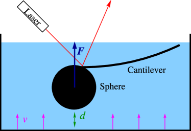
Figure 1: A sketch of a slip measurement based on a modified atomic force microscope (AFM). For technical reasons the surface is moved with the velocity $v$ towards the sphere which is attached to the cantilever of the AFM. The laser is used to measure the bending of the cantilever which can be related to the drag force $F$.

In general it should be noted that a significant dispersion of the slip measurements reported in the literature can be observed even in similar experimental systems (see ??). This is due to the large amount of unknown or uncontrolled parameters. For example, observed slip lengths vary between a few nanometres as reported by ? and micrometers as shown in ? and while some authors like  ??? find a dependence of the slip on the flow velocity, others like ?? do not.

The large variety of different experimental results to some extent has its origin in surface-fluid interactions. Their properties and thus their influence on the experimental results are often unknown and difficult to quantify. In addition there are many influences that lead to the same effect in a given experimental setup as intrinsic boundary slip – as for example a fluid layer with lower viscosity than the bulk viscosity near the boundary. Unless one is able to resolve the properties of this boundary layer it cannot be distinguished from true or intrinsic slip. Such effects can be categorized as apparent slip.

In the literature a large variety of different effects leading to an apparent slip can be found. However, detailed experimental studies are often difficult or even impossible. Here computer simulations can be utilized to predict the influence of effects like surface wettability or roughness. Most recent simulations apply molecular dynamics and report increasing slip with decreasing liquid density (see ?) or liquid-solid interactions (see ??), while slip decreases with increasing pressure (see ?). These simulations are usually limited to some tens of thousands of particles, length scales of the order of nanometres and time scales of the order of nanoseconds. Also, shear rates are usually orders of magnitude higher than in any experiment (see ?). Due to the small accessible time and length scales of molecular dynamics simulations, mesoscopic simulation methods like the lattice Boltzmann method are highly applicable for the simulation of microfluidic experiments. For a simple flow setup like Poiseuille or Couette flow several investigations of slip models have been published by ?????, but investigations for more complex flows are rare.

In this paper lattice Boltzmann simulations of AFM based experiments are presented. We focus on demonstrating that our method is able to reproduce the theoretical prediction for a simple no-slip case and investigate its limits. It is then possible to use the results to investigate the influence of different parameters. Such parameters can include an interaction between the sphere and the boundary, surface roughness or hydrophobicity. While the case of roughness is investigated in ?, further studies will be shown in future publications. Microscopic origins of slip caused by the molecular details of the fluid and surface cannot be treated with a continuum method and are beyond the scope of the current paper.

The remainder of this paper is arranged as follows: after this introduction we describe the theoretical background and our simulation method. Then we show that the method is able to reproduce the theoretical predictions with great accuracy. Further, we investigate the influence of finite size effects. We determine the minimum system size and resolution of the discretization required to push the finite size effects below an acceptable limit and demonstrate the limits of the simulation method.

2 Theoretical background

In this section the commonly used theory is summarized. The Reynolds lubrication force is given by Eq.1.4. For larger distances $d$ between the surface of the sphere and the approached boundary this force does not converge towards the Stokes drag force ${\bf F}_{\rm St}=6\pi\mu{\bf v}R$ for a sphere moving freely in a fluid. Therefore this simple equation fails in cases of larger separations $d$, where the Stokes force is not sufficiently small to be neglected. The system can be described accurately by the theory of ? and ?. The base of the theory is a solution for two spheres approaching each other with the same rate. By transforming the coordinates, applying symmetry arguments and setting the radius of one of the spheres to infinity one arrives at a fast converging sum for the drag force acting on the sphere:

$${\bf F}_{\rm Ma}=6\pi\mu{\bf v}R\lambda_{1},$$ (2.1)

with

$$\!\!\!\!\!\!\!\!\!\!\!\lambda_{1}=-\frac{1}{3}\sinh\xi$$

$$\!\!\!\!\!\!\!\!\!\!\!\times\left(\sum^{\infty}_{n=1}\frac{n(n+1)\left[8e^{(2n+1)\xi}+2(2n+3)(2n-1)\right]}{(2n-1)(2n+3)[4\sinh^{2}(n+\frac{1}{2})\xi-(2n+1)^{2}\sinh^{2}\xi]}\right.$$

$$\!\!\!\!\!\!\!\left.-\sum^{\infty}_{n=1}\frac{n(n+1)\left[(2n+1)(2n-1)e^{2\xi}-(2n+1)(2n+3)e^{-2\xi}\right]}{(2n-1)(2n+3)[4\sinh^{2}(n+\frac{1}{2})\xi-(2n+1)^{2}\sinh^{2}\xi]}\right),$$

where $\cosh\xi=(d-R)/R$. The term given by $\lambda_{1}$ cannot be treated analytically. Thus, we evaluate $\lambda_{1}$ numerically with a convergence of $10^{-10}$. A more practical approximation of (2.1) is given in the same paper by ?:

$$F(d)=6\pi\mu Rv\left(\frac{9}{8}\frac{R}{d}+1\right)$$ (2.2)

Here one can easily see that the force converges towards the Stokes force for an infinite distance $d$ and towards the Reynolds lubrication (1.4) for small separations $d$.

As stated above, to measure the slip length $b$ experiments apply a correction $f^{*}$ that takes into account the surface properties so that $F_{b}=f^{*}F(d)$. The correction function $f^{*}$ is given by Eq. 1.6. This equation is valid for a perfectly flat surface with finite slip, but it does not allow one to distinguish between slip and other effects like surface roughness. Therefore it is of importance to perform computer simulations which have the advantage that all relevant parameters can be changed independently without modifying anything else in the setup. Thus, the influence of every single modification can be studied in order to present estimates of the influence on the measured slip lengths. The first step in this process is to validate the simulation method and to understand its merits and flaws. In general most computer simulations suffer from the fact that only a small system can be described and that one is usually not able to simulate the whole experimental system in full detail. For this reason it is mandatory to understand which resolution of the problem is required to keep finite size effects under control and to cover the important physics correctly.

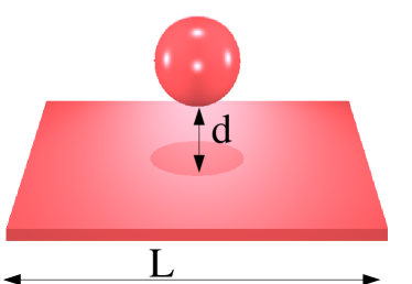
Figure 2: A sketch of the simulated system. The distance between the surface and the sphere is $d$ and the system length is $L$. The surrounding fluid is not shown.

In Fig. 2 a sketch of the simulated system is shown. A sphere embedded in a surrounding fluid is simulated. While the sphere approaches a surface the force acting on it is recorded. We perform simulations with different sphere radius $R$ and different system length $L$ to investigate finite size effects. For simplicity we set the $x$ and $z$ dimension to the same value $L$ and keep the propagation dimension $y$ constant at $512$ lattice units. A typical approach to limit finite size effects is to use periodic boundary conditions. However in such a system the sphere then interacts with its periodic images. ? gives a theoretical solution for the drag force of a sphere in a periodic array as it appears if all boundaries are periodic:

$${\bf F}_{\rm Ha}=\frac{\bf F_{\rm St}}{1-2.83a+4.19a^{3}-27.4a^{7}+O(a^{9})}$$ (2.3)

Here, $a=R/L$ is the ratio between the radius of the sphere $R$ and the system length $L$. The case we are dealing with in this paper is different and more complex due to a broken symmetry caused by the approached surface. For the approximation given by (2.3) the main contribution of the periodic interaction is between the periodic images in front and behind the sphere. Due to the rigid boundary, these are not present in our case.

Besides a finite simulated volume most simulation methods utilize a finite discretization of the simulated objects, i.e. the sphere in our case. This means that the finite size and the resolution influence the result of a simulation. However, it is usually possible to limit the influence of finite size effects and the loss of accuracy by discretization if those errors are known and taken into account properly. Therefore, we study the finite size effects in a simulation of a sphere in a periodic system approaching a rigid no slip boundary and investigate how different resolutions of the sphere influence the force acting on it.

3 Simulation Method

The simulation method used to study microfluidic devices has to be chosen carefully. While Navier-Stokes solvers are able to cover most problems in fluid dynamics, they lack the possibility to include the influence of molecular interactions as needed to model boundary slip. Molecular dynamics simulations (MD) are the best choice to simulate the fluid-wall interaction, but computer power today is not sufficient to simulate length and time scales necessary to achieve orders of magnitude which are relevant for experiments. However, boundary slip with a slip length $b$ of the order of many molecular diameters $\sigma$ has been studied with molecular dynamics simulations by various authors like ????.

In this paper we use the lattice Boltzmann method, where one discretizes the Boltzmann kinetic equation

$$\left[\frac{\partial}{\partial t}+{\bf u}\nabla_{x}+\frac{\hat{\bf F}}{m}\nabla_{u}\right]n({\bf x},{\bf u},t)={\bf\Omega}$$ (3.1)

on a lattice. $n({\bf x,u},t)$ indicates the probability to find a single particle with mass $m$ and velocity ${\bf u}$ at the time $t$ and position ${\bf x}$. $\hat{\bf F}$ accounts for external forces. The derivatives represent simple propagation of a single particle in real and velocity space whereas the collision operator ${\bf\Omega}$ takes into account molecular collisions in which a particle changes its momentum due to a collision with another particle. Further, the collision operator drives the distribution $n$ towards an equilibrium distribution $n^{eq}$.

In the lattice Boltzmann method time, positions, and velocity space are discretized on a lattice in the following way. The distribution $n$ is only present on lattice nodes ${\bf x}_{k}$. The velocity space is discretized so that in one discrete timestep $\delta t$ the particles travel with the discrete velocities ${\bf c}_{i}$ towards the nearest and next nearest neighbours ${\bf x}_{k}+{\bf c}_{i}\delta t$. Since a large proportion of the distribution stays at the same lattice node a rest velocity ${\bf c}_{0}$ is required. ${\bf c}_{0}$ represents particles not moving to a neighboring site. In short we operate on a three dimensional grid with 19 velocities ($i=0..18$) which is commonly referred to as D3Q19. After the streaming of the population density, the population on each lattice node is relaxed towards an equilibrium such that mass and momentum are conserved. It can be shown by a Chapman-Enskog procedure that such a simulation method reproduces the Navier-Stokes equation, ?. In the lattice Boltzmann method the time $t$ is discretized in time steps $\delta t$, the position ${\bf x}$ is discretized in units of distance between neighbouring lattice cells, and the velocity ${\bf u}$ is discretized using the velocity vectors ${\bf c}_{i}$. These form the natural lattice units of the method which are used in this paper if not stated otherwise.

The implementation we are using originates from ?. It applies a so called multi relaxation time collision operator. The distribution $n$ is transformed via a transformation matrix $T$ into the space of the moments $m_{j}$ of the distribution. A very accessible feature of this approach is that some of the moments $m_{j}$ have a physical meaning as for example the density

$$\rho=m_{0}=\sum_{i}n_{i}$$ (3.2)

or the momentum in each direction $x,y,z$,

$$m_{1,2,3}={\bf e}_{1,2,3}\sum_{i}n_{i}{\bf c}_{i}.$$ (3.3)

${\bf e}_{1,2,3}$ is the unit vector in Cartesian directions. The moments $m_{j}$ relax with an individual rate $S_{j}$ towards the equilibrium $m_{j}^{eq}$. The equilibrium distribution $m^{eq}$ conserves mass $m_{0}$ and momentum $m_{1,2,3}$ and is a discretized version of the Maxwell distribution. Thus the lattice Boltzmann equation (3.1) can be written as

$$n({\bf x}_{k}+{\bf c}_{i}\delta t,{\bf c}_{i},t+\delta t)-n({\bf x}_{k},{\bf c}_{i},t)$$

$$={T_{i}^{j}}^{-1}S_{j}[m_{j}({\bf x}_{k},t)-m_{j}^{eq}].$$ (3.4)

The multi relaxation time approach has several advantages compared to other lattice Boltzmann schemes. These include a higher precision at solid boundaries and the direct accessibility of the moments which represent physical properties. The latter can be utilized to easily implement thermal fluctuations or external and internal forces (see ?).

A feature of the implementation we are using is the possibility to simulate particles suspended in fluid. The simulation method is described extensively in the literature (see ????). Therefore only a brief description is given here. The movement of the particles is described by a simple molecular dynamics algorithm. However it should be noted here that we simulate a sphere moving with a constant velocity. Therefore any forces acting on the sphere do not influence its movement. The fluid-particle interaction is achieved by the solid-fluid boundary interaction acting on the surface of the sphere. When the sphere is discretized on the lattice all lattice sites inside the sphere are marked as boundary nodes with a moving wall boundary condition. This boundary condition at the solid-fluid interface is constructed in such a way that there is as much momentum transferred to the fluid as required for the fluid velocity to match the boundary velocity ${\bf v}_{b}$ of the particle. The center of mass velocity of the particle and the rotation are taken into account. This way the transfered momentum and thus the hydrodynamic force acting on the sphere are known. Technically speaking a link bounce back boundary condition is implemented for the solid nodes together with a momentum transfer term. The link bounce back implies that the distributions that would move inside the boundary with the velocity ${\bf c}_{i}$ are reversed in direction with opposite velocity ${\bf c}_{k}$.

$$\!\!\!\!\!\!\!\!\!\!\!\!\!n({\bf x}+{\bf c}_{i}\delta t,{\bf c}_{i},t+\delta t) \!\!\!=\!\!\! n({\bf x}+{\bf c}_{i}\delta t,{\bf c}_{k},t)\!+\!\frac{2a^{{\bf c}_{i}}\rho{\bf v}_{b}{\bf c}_{i}}{c_{s}^{2}}$$ (3.5)

$$n({\bf x},{\bf c}_{k},t+\delta t) \!\!\!=\!\!\! n({\bf x},{\bf c}_{i},t)\!+\!\frac{2a^{{\bf c}_{i}}\rho{\bf v}_{b}c_{i}}{c_{s}^{2}}$$ (3.6)

Here, $a^{{\bf c}_{i}}$ are weight factors taking into account the different lengths of the lattice vectors.

While the center of mass of the sphere moves, new lattice nodes become part of the particle, while others become fluid. Therefore particles do not perform a continuous movement but rather small jumps. After each jump the fluid is out of equilibrium but relaxes very quickly back to the quasi static state. In order to average out statistical fluctuations imposed by the discrete movement of the particle, one has to average the recorded force over several time steps. We choose to average over intervals of $999$ steps.

If not stated otherwise the simulation parameters are ${v}=0.001$, $\mu=0.1$ and the radius is varied between $R=4$ and $R=16$. The approached boundary is a plain no-slip wall which is realized by a mid grid bounce back boundary condition.

Along the open sides periodic boundary conditions are applied so that the sphere can interact with its mirror leading to the to be avoided finite size effects. As noted in Fig. 2 the length of the system in $x$ and $y$ direction is $L$. The size of the simulation volume is varied to explore the influence of finite size effects.

4 Results

In this contribution we vary the system length $L$ and the radius of the sphere $R$. A major contribution to the finite size effects is the interaction of the sphere with its periodic image. Therefore a larger system length should reduce this effect dramatically. However when the hydrodynamic influence of the wall becomes larger finite size effects become smaller. This can be explained by the fact that the friction at the boundary suppresses the hydrodynamic interaction of the particle with its periodic image. Instead the dominant interaction is between the particle and the surface. It is mandatory for a better understanding of the system to learn how these finite size effects can be described, quantified, and controlled.

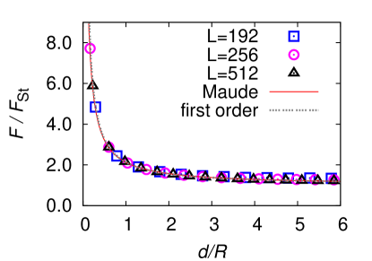
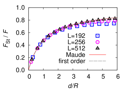
Figure 3: Normalized drag force $\frac{F}{F_{St}}$ and the inverted normalized drag force $\frac{F_{St}}{F}$ versus the normalized distance $d/R$ for different system lengths $L$. The radius of the sphere is fixed at $R=16$. The deviation for $L=192$ is significant at larger radii, but can be neglected for small distances. For $L=512$ there is nearly no deviation from the exact solution of Maude (2.1). In addition the deviation of the first order approximation (2.2) is below $1\%$ for $d>R/2$.

First we study a system with a constant sphere radius $R=16$ and varying system length $L$. In Fig. 3 the drag force ${F}$ normalized by the Stokes force ${F}_{\rm St}=6\pi\mu{v}R$ and the inverse normalized drag force are plotted. In the inversed case the deviations for the larger distance $d$ can be seen more clearly. Fig. 3 shows that the deviation for the small system $L=192$ close to the wall is very small, however the force does not converge to the Stokes force ${F}_{\rm St}$. Here effects similar to the one reported by Hasimoto (2.3) appear: for a smaller separation $d$ the force decays with $\frac{1}{d}$ while it approaches a constant value for large $d$. The constant values should be given by the Stokes force ${F}_{\rm St}$, but can be larger due to the interaction with the periodic image. In the $1/F$ plots it can be seen that the deviation is not a constant offset or factor but rather starts at a critical value of $d/R$. From there the force quickly starts to approach a constant value.

In Fig. 4 the relative error $E=\frac{F-F_{Maude}}{F}$ is plotted for different system sizes $L$ and a constant radius $R$. The error for the largest system $L=512$ in Fig 4 is constantly below $1\%$ for larger distances. At distances less than $d<R/2$ the error rises due to the insufficient resolution of the fluid filled volume between the surface of the sphere and the boundary. Another possible effect is the fact that the sphere rather jumps over the lattice than performing a continuous movement. Additionally it can be seen that for distances less than $d=R$ the error for the different system sizes $L$ collapses. The reason is that for smaller distances the lubrication effect which is independent of the system length $L$ dominates the free flow and therefore suppresses finite size effects due to the periodic image. The deviation that can be seen in the plot at the large $d$ has its origin in the transient. Since the fluid is at rest at the start of the simulation and it takes some time to reach a steady state this can only be avoided by longer simulations. An interesting fact to point out is that the deviation between the Maude solution and the first order approximation is below $1\%$.

Figure 4: Symbols denote the relative error $E=\frac{F-F_{Maude}}{F_{Maude}}$ in % versus the normalized distance $d/R$ for different system sizes $L$. The line shows the first order approximation. As expected the error close to the wall deviates due to the discretization of the small distance $d$. The error becomes larger for large $d$ due to the influence of the periodic image.

Since the sphere is discretized on the lattice it is important to understand if this discretization has an effect on the drag force. Therefore we perform simulations with a radius of $R={4,8,16}$ at a constant ratio $R/L=1/32$ between the radius and the system length. Fig. 5 depicts the normalized drag force $\frac{F}{F_{\rm St}}$ and the inverted normalized drag force $\frac{F_{\rm St}}{F}$ versus the normalized distance $d/R$ for different radii $R$. It can be seen that the discretization of the sphere has little influence on the measured force.

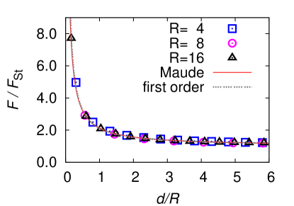
Figure 5: Normalized drag force $\frac{F}{F_{\rm St}}$ and the inverted normalized drag force $\frac{F_{\rm St}}{F}$ versus the normalized distance $d/R$ for different radii $R$ but constant ratio $R/L=1/32$

Fig. 6 shows the relative error $E$ for different radii. For all radii the finite size effects due to the periodic image are negligible since the ratio between $R/L$ is sufficiently small. The deviation from the Maude theory for separations $d>R$ are below $2\%$ for all radii. Therefore one has to concentrate on the small distances $d$ where significant deviations appear. In our case this distance is better resolved for larger $R$ (note that in the plot the normalized distance is shown). In addition the resolution of the sphere is better for larger $R$. For $R=4$ the deviation is more noisy and here the discretization really has an effect on the drag force ${\bf F}$. However, even a such roughly discretized sphere reproduces the expected result surprisingly well. This can probably be explained by averaging out of discretization artefacts due to the time and space averaging performed in the simulations. Additionally there should be three or more lattice sites between the surface of the sphere and the boundary. If that is not the case the hydrodynamic interaction is not resolved sufficiently. If the distance between surface and sphere is smaller than half a lattice spacing the two surfaces merge and the method fails. Hence it is advantageous to choose a large radius in order to be able to reduce the relative distance to the boundary (in units of the sphere radius) or to resolve a possible surface structure.

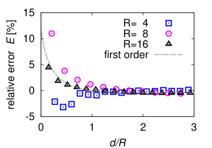
Figure 6: Relative error $E=\frac{F-F_{\rm Maude}}{F_{\rm Maude}}$ in % versus the normalized distance $d/R$ for different radii $L$ at a constant ratio $R/L=\frac{4}{128}$ (symbols). As expected the error close to the wall deviates, due to the discretization of the small distance $d$. For $R=4$ the deviation fluctuates due to the low resolution but for $R=16$ it follows the first order approximation. The line corresponds to the first order approximation.

For $R\geq 8$ the deviations have a regular shape and follow the deviation for the first order approximation. The trend to follow the first order approximation is stronger for $R=16$ but here the noise is reduced further and all errors seem to be systematic. Therefore the deviation has to be described as a systematic error of the method that has its origin in the “jumping-standing” like movement of the sphere. The first order approximation is a quasi static approximation and represents the actual simulated movement more correctly than the theory of Maude.

It should be noted that the finite size effects for $R=16$ and $R/L=1/16$ due to the interaction with the periodic image are much more significant than the discretization effect. By choosing a large simulation volume, a radius $R>8$ and focusing on the force for separations $d<2R$ one can reduce those effects to a deviation of the measured force from the theoretically predicted value of less than $1\%$.

5 Conclusion

Lattice Boltzmann simulations of a high-speed drainage of liquid films squeezed between a sphere and a smooth no-slip surface have been presented. We have shown that the solution of Maude (2.1) can be reproduced and demonstrated that at a ratio $R/L=1/32$ finite size effects are below $2\%$ and thus can be neglected near the boundary. We have also demonstrated that a sphere radius of $R=8$ provides a sufficiently well resolved representation of the sphere. Based on this calibration it is possible to investigate the influence of different surface properties such as roughness and slip on the drag force on AFM based slip measurements.