On Generalizations of Network Design Problems
with Degree Bounds

Abstract

Iterative rounding and relaxation have arguably become the method of choice in dealing with unconstrained and constrained network design problems. In this paper we extend the scope of the iterative relaxation method in two directions: (1) by handling more complex degree constraints in the minimum spanning tree problem (namely laminar crossing spanning tree), and (2) by incorporating ‘degree bounds’ in other combinatorial optimization problems such as matroid intersection and lattice polyhedra. We give new or improved approximation algorithms, hardness results, and integrality gaps for these problems.

• Our main result is a $(1,b+O(\log n))$-approximation algorithm for the minimum crossing spanning tree (MCST) problem with laminar degree constraints. The laminar MCST problem is a natural generalization of the well-studied bounded-degree MST, and is a special case of general crossing spanning tree. We also give an additive $\Omega(\log^{\alpha}m)$ hardness of approximation for general MCST, even in the absence of costs ($\alpha>0$ is a fixed constant, and $m$ is the number of degree constraints).

• We then consider the crossing contra-polymatroid intersection problem and obtain a $(2,2b+\Delta-1)$-approximation algorithm, where $\Delta$ is the maximum element frequency. This models for example the degree-bounded spanning-set intersection in two matroids. Finally, we introduce the crossing lattice polyhedra problem, and obtain a $(1,b+2\Delta-1)$ approximation under certain condition. This result provides a unified framework and common generalization of various problems studied previously, such as degree bounded matroids.

1 Introduction

Iterative rounding and relaxation have arguably become the method of choice in dealing with unconstrained and constrained network design problems. Starting with Jain’s elegant iterative rounding scheme for the generalized Steiner network problem in [18], an extension of this technique (iterative relaxation) has more recently lead to breakthrough results in the area of constrained network design, where a number of linear constraints are added to a classical network design problem. Such constraints arise naturally in a wide variety of practical applications, and model limitations in processing power, bandwidth or budget. The design of powerful techniques to deal with these problems is therefore an important goal.

The most widely studied constrained network design problem is the minimum-cost degree-bounded spanning tree problem. In an instance of this problem, we are given an undirected graph, non-negative costs for the edges, and positive, integral degree-bounds for each of the nodes. The problem is easily seen to be NP-hard, even in the absence of edge-costs, since finding a spanning tree with maximum degree two is equivalent to finding a Hamiltonian Path. A variety of techniques have been applied to this problem [8, 9, 15, 21, 22, 27, 28], culminating in Singh and Lau’s breakthrough result in [31]. They presented an algorithm that computes a spanning tree of at most optimum cost whose degree at each vertex $v$ exceeds its bound by at most $1$, using the iterative relaxation framework developed in [24, 31].

The iterative relaxation technique has been applied to several constrained network design problems: spanning tree [31], survivable network design [24, 25], directed graphs with intersecting and crossing super-modular connectivity [24, 4]. It has also been applied to degree bounded versions of matroids and submodular flow [19].

In this paper we further extend the applicability of iterative relaxation, and obtain new or improved bicriteria approximation results for minimum crossing spanning tree (MCST), crossing contra-polymatroid intersection, and crossing lattice polyhedra. We also provide some hardness results and integrality gaps for these problems.

Notation. As is usual, when dealing with an undirected graph $G=(V,E)$, for any $S\subseteq V$ we let $\delta_{G}(S):=\{(u,v)\in E\mid u\in S,~{}v\not\in S\}$. When the graph is clear from context, the subscript is dropped. A collection $\{U_{1},\cdots,U_{t}\}$ of vertex-sets is called laminar if for every pair $U_{i},U_{j}$ in this collection, we have $U_{i}\subseteq U_{j}$, $U_{j}\subseteq U_{i}$, or $U_{i}\cap U_{j}=\emptyset$. A $(\rho,f(b))$ approximation for minimum cost degree bounded problems refers to a solution that (1) has cost at most $\rho$ times the optimum that satisfies the degree bounds, and (2) satisfies the relaxed degree constraints in which a bound $b$ is replaced with a bound $f(b)$.

1.1 Our Results, Techniques and Paper Outline

Laminar MCST.

Our main result is for a natural generalization of bounded-degree MST (called Laminar Minimum Crossing Spanning Tree or laminar MCST), where we are given an edge-weighted undirected graph with a laminar family ${\cal L}=\{S_{i}\}_{i=1}^{m}$ of vertex-sets having bounds $\{b_{i}\}_{i=1}^{m}$; and the goal is to compute a spanning tree of minimum cost that contains at most $b_{i}$ edges from $\delta(S_{i})$ for each $i\in[m]$.

The motivation behind this problem is in designing a network where there is a hierarchy (i.e. laminar family) of service providers that control nodes (i.e. vertices). The number of edges crossing the boundary of any service provider (i.e. its vertex-cut) represents some cost to this provider, and is therefore limited. The laminar MCST problem precisely models the question of connecting all nodes in the network while satisfying bounds imposed by all the service providers.

From a theoretical viewpoint, cut systems induced by laminar families are well studied, and are known to display rich structure. For example, one-way cut-incidence matrices are matrices whose rows are incidence vectors of directed cuts induced by the vertex-sets of a laminar family; It is well known (e.g., see [23]) that such matrices are totally unimodular. Using the laminar structure of degree-constraints and the iterative relaxation framework, we obtain the following main result, and present its proof in Section 2.

Theorem 1

There is a polynomial time $(1,b+O(\log n))$ bicriteria approximation algorithm for laminar MCST. That is, the cost is no more than the optimum cost and the degree violation is at most additive $O(\log n)$. This guarantee is relative to the natural LP relaxation.

This guarantee is substantially stronger than what follows from known results for the general minimum crossing spanning tree (MCST) problem: where the degree bounds could be on arbitrary edge-subsets $E_{1},\ldots,E_{m}$. In particular, for general MCST a $(1,b+\Delta-1)$ [4, 19] is known where $\Delta$ is the maximum number of degree-bounds an edge appears in. However, this guarantee is not useful for laminar MCST as $\Delta$ can be as large as $\Omega(n)$ in this case. If a multiplicative factor in the degree violation is allowed, Chekuri et al. [11] recently gave a very elegant $\left(1,(1+\epsilon)b+O(\frac{1}{\epsilon}\log m)\right)$ guarantee (which subsumes the previous best $(O(\log n),O(\log m)\,b)$ [6] result). However, these results also cannot be used to obtain a small additive violation, especially if $b$ is large. In particular, both the results [6, 11] for general MCST are based on the natural LP relaxation, for which there is an integrality gap of $b+\Omega(\sqrt{n})$ even without regard to costs and when $m=O(n)$ [30] (see also Section 3.2). On the other hand, Theorem 1 shows that a purely additive $O(\log n)$ guarantee on degree (relative to the LP relaxation and even in presence of costs) is indeed achievable for MCST, when the degree-bounds arise from a laminar cut-family.

The algorithm in Theorem 1 is based on iterative relaxation and uses two main new ideas. Firstly, we drop a carefully chosen constant fraction of degree-constraints in each iteration. This is crucial as it can be shown that dropping one constraint at a time as in the usual applications of iterative relaxation can indeed lead to a degree violation of $\Omega(\Delta)$. Secondly, the algorithm does not just drop degree constraints, but in some iterations it also generates new degree constraints, by merging existing degree constraints.

All previous applications of iterative relaxation to constrained network design treat connectivity and degree constraints rather asymmetrically. While the structure of the connectivity constraints of the underlying LP is used crucially (e.g., in the ubiquitous uncrossing argument), the handling of degree constraints is remarkably simple. Constraints are dropped one by one, and the final performance of the algorithm is good only if the number of side constraints is small (e.g., in recent work by Grandoni et al. [16]), or if their structure is simple (e.g., if the ‘frequency’ of each element is small). In contrast, our algorithm for laminar MCST exploits the structure of degree constraints in a non-trivial manner.

Hardness Results.

We obtain the following hardness of approximation for the general MCST problem (and its matroid counterpart). In particular this rules out any algorithm for MCST that has additive constant degree violation, even without regard to costs.

Theorem 2

Unless $\mathcal{NP}$ has quasi-polynomial time algorithms, the MCST problem admits no polynomial time $O(\log^{\alpha}m)$ additive approximation for the degree bounds for some constant $\alpha>0$; this holds even when there are no costs.

The proof for this theorem is given in Section 3, and uses a a two-step reduction from the well-known Label Cover problem. First, we show hardness for a uniform matroid instance. In a second step, we then demonstrate how this implies the result for MCST claimed in Theorem 2.

Note that our hardness bound nearly matches the result obtained by Chekuri et al. in [11]. We note however that in terms of purely additive degree guarantees, a large gap remains. As noted above, there is a much stronger lower bound of $b+\Omega(\sqrt{n})$ for LP-based algorithms [30] (even without regard to costs), which is based on discrepancy. In light of the small number of known hardness results for discrepancy type problems, it is unclear how our bounds for MCST could be strengthened.

An interesting consequence of the hardness result in Theorem 2 is for the robust (or min-max) $k$-median problem [1]. In this problem, there are $m$ different client-sets in a metric and the goal is to open $k$ facilities that are simultaneously good (in terms of the $k$-median objective) for all the client-sets. Anthony et al. [1] obtained a logarithmic approximation algorithm for this problem, and showed that it is hard to approximate better than factor $2$. The following result shows that the robust $k$-median problem is indeed harder to approximate than usual $k$-median, for which $O(1)$-approximations are known [7, 3]. We present its proof in Section 3.1.

Corollary 3

Robust $k$-median is $\Omega(\log^{\alpha}m)$-hard to approximate even on uniform metrics (for some fixed constant $\alpha>0$), assuming $\mathcal{NP}$ does not have quasi-polynomial time algorithms.

Degree Bounds in More General Settings.

We consider crossing versions of other classic combinatorial optimization problems, namely contra-polymatroid intersection and lattice polyhedra [29].

Definition 4 (Minimum crossing contra-polymatroid intersection problem)

Let $r_{1},r_{2}:2^{E}\to\mathbb{Z}$ be two supermodular functions, $c:E\to\mathbb{R}_{+}$ and $\{E_{i}\}_{i\in I}$ be a collection of subsets of $E$ with corresponding bounds $\{b_{i}\}_{i\in I}$. Then the goal is to minimize:

$$\{c^{T}x~{}\big{|}\quad x(S)\geq\max\{r_{1}(S),r_{2}(S)\},\forall~{}S\subseteq E;$$

$$x(E_{i})\leq b_{i},~{}~{}\forall~{}i\in I;\quad x\in\{0,1\}^{E}\}.$$

In particular, this definition captures the degree-bounded version of spanning-set intersection in two matroids (for eg. the bipartite edge-cover problem). We note that this definition does not capture alternate notions of matroid intersection, such as intersection of bases in two matroids; hence it does not apply to the degree-bounded arborescence problem. 

Let $\Delta=\max_{e\in E}|\{i\in[m]\mid e\in E_{i}\}|$ be the largest number of sets $E_{i}$ that any element of $E$ belongs to, and refer to it as frequency. The proof of this theorem can be found in Section 4.

Theorem 5

Any optimal basic solution $x^{*}$ of the linear relaxation of the minimum crossing contra-polymatroid intersection problem can be rounded into an integral solution $\hat{x}$ such that:

$$\hat{x}(S)\geq\max\{r_{1}(S),r_{2}(S)\},\,\,\forall S\subseteq E;\qquad\hat{x}(E_{i})\leq 2b_{i}+\Delta-1,\,\,\forall i\in I;\quad\mbox{and}\quad c^{T}\hat{x}\leq 2c^{T}x^{*}.$$

The algorithm for this theorem again uses iterative relaxation, and its proof is based on a ‘fractional token’ counting argument similar to the one used in [4]. We also observe that the natural iterative relaxation steps are insufficient to obtain a better approximation guarantee.

Crossing Lattice Polyhedra. Classical lattice polyhedra form a unified framework for various discrete optimization problems and go back to Hoffman and Schwartz [17] who proved their integrality. They are polyhedra of type

$$\{x\in[0,1]^{E}\mid x(\rho(S))\geq r(S),\quad\forall S\in\mathcal{F}\}$$

where $\mathcal{F}$ is a consecutive submodular lattice, $\rho:\mathcal{F}\rightarrow 2^{E}$ is a mapping from $\mathcal{F}$ to subsets of the ground-set $E$, and $r\in\mathbb{R}^{\mathcal{F}}$ is supermodular. A key property of lattice polyhedra is that the uncrossing technique can be applied which turns out to be crucial in almost all iterative relaxation approaches for optimization problems with degree bounds. We refer the reader to [29] for a more comprehensive treatment of this subject.

We generalize our work further to crossing lattice polyhedra which arise from classical lattice polyhedra by adding “degree-constraints” of the form $a_{i}\leq x(E_{i})\leq b_{i}$ for a given collection $\{E_{i}\subseteq E\mid i\in I\}$ and lower and upper bounds $a,b\in\mathbb{R}^{I}$. We mention two (of several) examples which are covered by this model:

Example 1: Crossing matroid basis. Here $\mathcal{F}=2^{E}$, $\rho$ is the identity map, and the partial order in $\mathcal{F}$ is the canonical one that is induced by set inclusion. Function $r:2^{E}\rightarrow\mathbb{N}$ is defined as $r(S)=\sf rank(V)-\sf rank(V\setminus S)$; where $E$ is the ground-set of the matroid and $\sf rank$  is its rank function. The crossing matroid basis problem finds the minimum cost basis in the matroid satisfying degree bounds.

Example 2: Crossing planar min cut. Let $G=(V,E)$ be a (directed or undirected) $s,t$-planar graph (along with an embedding) with $s,t\in V$. Here elements of $\mathcal{F}$ correspond to $s$-$t$ paths in $G$ ($\rho$ maps each element of $\mathcal{F}$ to the edge-set of that $s-t$ path), and the partial order in $\mathcal{F}$ relates paths where one is below/above the other in the planar embedding of $G$. The rank function is the constant all-ones function. The crossing planar min-cut problem involves finding a minimum cost $s-t$ cut in $G$ that obeys the degree bounds.

We can show that the standard LP relaxation for the general crossing lattice polyhedron problem is weak; in Section 5.1 we give instances of crossing planar min-cut (i.e., Example 2 above) where the LP-relaxation is feasible, but any integral solution violates some degree-bound by $\Omega(\sqrt{n})$. For this reason, we henceforth focus on a restricted class of crossing lattice polyhedra in which the underlying lattice $(\mathcal{F},\leq)$ satisfies the following monotonicity property

$$(*)\quad S<T\implies|\rho(S)|<|\rho(T)|\qquad\forall~{}S,T\in\mathcal{F}.$$

We obtain the following theorem whose proof is given in Section 5.

Theorem 6

For any instance of the crossing lattice polyhedron problem in which $\mathcal{F}$ satisfies property $(*)$, there exists an algorithm that computes an integral solution of cost at most the optimal, where all rank constraints are satisfied, and each degree bound is violated by at most an additive $2\Delta-1$.

We note that the above property $(*)$ is satisfied for matroids, and hence Theorem 6 matches the previously best-known bound [19] for degree bounded matroids (with both upper/lower bounds). Also note that property $(*)$ holds whenever $\mathcal{F}$ is ordered by inclusion. In this special case, we can improve the result to an additive $\Delta-1$ approximation if only upper bounds are given.

1.2 Related Work

As mentioned earlier, the basic bounded-degree MST problem has been extensively studied [8, 9, 15, 21, 22, 27, 28, 31]. The iterative relaxation technique for degree-constrained problems was developed in [24, 31].

MCST was first introduced by Bilo et al. [6], who presented a randomized-rounding algorithm that computes a tree of cost $O(\log n)$ times the optimum where each degree constraint is violated by a multiplicative $O(\log n)$ factor and an additive $O(\log m)$ term. Subsequently, Bansal et al. [4] gave an algorithm that attains an optimal cost guarantee and an additive $\Delta-1$ guarantee on degree; recall that $\Delta$ is the maximum number of degree constraints that an edge lies in. This algorithm used iterative relaxation as its main tool. Recently, Chekuri et al. [11] obtained an improved $\left(1,(1+\epsilon)b+O(\frac{1}{\epsilon}\log m)\right)$ approximation algorithm for MCST, for any $\epsilon>0$; this algorithm is based on pipage rounding.

The minimum crossing matroid basis problem was introduced in [19], where the authors used iterative relaxation to obtain (1) $(1,b+\Delta-1)$-approximation when there are only upper bounds on degree, and (2) $(1,b+2\Delta-1)$-approximation in the presence of both upper and lowed degree-bounds. The [11] result also holds in this matroid setting. [19] also considered a degree-bounded version of the submodular flow problem and gave a $(1,b+1)$ approximation guarantee.

The bounded-degree arborescence problem was considered in Lau et al. [24], where a $(2,2b+2)$ approximation guarantee was obtained. Subsequently Bansal et al. [4] designed an algorithm that for any $0<\epsilon\leq 1/2$, achieves a $(1/\epsilon,b_{v}/(1-\epsilon)+4)$ approximation guarantee. They also showed that this guarantee is the best one can hope for via the natural LP relaxation (for every $0<\epsilon\leq 1/2$). In the absence of edge-costs,  [4] gave an algorithm that violates degree bounds by at most an additive two. Recently Nutov [26] studied the arborescence problem under weighted degree constraints, and gave a $(2,5b)$ approximation for it.

Lattice polyhedra were first investigated by Hoffman and Schwartz [17] and the natural LP relaxation was shown to be totally dual integral. Even though greedy-type algorithms are known for all examples mentioned earlier, so far no combinatorial algorithm has been found for lattice polyhedra in general. Two-phase greedy algorithms have been established only in cases where an underlying rank function satisfies a monotonicity property  [14], [12].

2 Crossing Spanning Tree with Laminar degree bounds

In this section we prove Theorem 1 by presenting an iterative relaxation-based algorithm with the stated performance guarantee. During its execution, the algorithm selects and deletes edges, and it modifies the given laminar family of degree bounds. A generic iteration starts with a subset $F$ of edges already picked in the solution, a subset $E$ of undecided edges, i.e., the edges not yet picked or dropped from the solution, a laminar family $\mathcal{L}$ on $V$, and residual degree bounds $b(S)$ for each $S\in\mathcal{L}$.

The laminar family $\mathcal{L}$ has a natural forest-like structure with nodes corresponding to each element of $\mathcal{L}$. A node $S\in\mathcal{L}$ is called the parent of node $C\in\mathcal{L}$ if $S$ is the inclusion-wise minimal set in $\mathcal{L}\setminus\{C\}$ that contains $C$; and $C$ is called a child of $S$. Node $D\in\mathcal{L}$ is called a grandchild of node $S\in\mathcal{L}$ if $S$ is the parent of $D$’s parent. Nodes $S,T\in\mathcal{L}$ are siblings if they have the same parent node. A node that has no parent is called root. The level of any node $S\in\mathcal{L}$ is the length of the path in this forest from $S$ to the root of its tree. We also maintain a linear ordering of the children of each $\mathcal{L}$-node. A subset $\mathcal{B}\subseteq\mathcal{L}$ is called consecutive if all nodes in $\mathcal{B}$ are siblings (with parent $S$) and they appear consecutively in the ordering of $S$’s children. In any iteration $(F,E,\mathcal{L},b)$, the algorithm solves the following LP relaxation of the residual problem.

$$\min\quad \sum_{e\in E}c_{e}x_{e}$$ (1)

s.t. $$x(E(V))=|V|-|F|-1$$

$$x(E(U))\leq|U|-|F(U)|-1\quad \forall U\subset V$$

$$x(\delta_{E}(S))\leq b(S) \forall S\in\mathcal{L}$$

$$x_{e}\geq 0\quad \forall e\in E$$

For any vertex-subset $W\subseteq V$ and edge-set $H$, we let $H(W):=\{(u,v)\in H\mid u,v\in W\}$ denote the edges induced on $W$; and $\delta_{H}(W):=\{(u,v)\in H\mid u\in W,~{}v\not\in W\}$ the set of edges crossing $W$. The first two sets of constraints are spanning tree constraints while the third set corresponds to the degree bounds. Let $x$ denote an optimal extreme point solution to this LP. By reducing degree bounds $b(S)$, if needed, we assume that $x$ satisfies all degree bounds at equality (the degree bounds may therefore be fractional-valued). Let $\alpha:=24$.

Definition 7

An edge $e\in E$ is said to be local for $S\in\mathcal{L}$ if $e$ has at least one end-point in $S$ but is neither in $E(C)$ nor in $\delta(C)\cap\delta(S)$ for any grandchild $C$ of $S$. Let $\mathrm{local}(S)$ denote the set of local edges for $S$. A node $S\in\mathcal{L}$ is said to be good if $|\mathrm{local}(S)|\leq\alpha$.

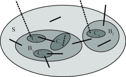
Figure 1: Example of local edges.

Figure 1 shows a set $S$, its children $B_{1}$ and $B_{2}$, and grand-children $C_{1},\ldots,C_{4}$; edges in $\mathrm{local}(S)$ are drawn solid, non-local ones are shown dashed.

Initially, $E$ is the set of edges in the given graph, $F\leftarrow\emptyset$, $\mathcal{L}$ is the original laminar family of vertex sets for which there are degree bounds, and an arbitrary linear ordering is chosen on the children of each node in $\mathcal{L}$. In a generic iteration $(F,E,\mathcal{L},b)$, the algorithm performs one of the following steps (see also Figure 2):

1. If $x_{e}=1$ for some edge $e\in E$ then $F\leftarrow F\cup\{e\}$, $E\leftarrow E\setminus\{e\}$, and set $b(S)\leftarrow b(S)-1$ for all $S\in\mathcal{L}$ with $e\in\delta(S)$.

2. If $x_{e}=0$ for some edge $e\in E$ then $E\leftarrow E\setminus\{e\}$.

3. DropN: Suppose there at least $|\mathcal{L}|/4$ good non-leaf nodes in $\mathcal{L}$. Then either odd-levels or even-levels contain a set $\mathcal{M}\subseteq\mathcal{L}$ of $|\mathcal{L}|/8$ good non-leaf nodes. Drop the degree bounds of all children of $\mathcal{M}$ and modify $\mathcal{L}$ accordingly. The ordering of siblings also extends naturally.

4. DropL: Suppose there are more than $|\mathcal{L}|/4$ good leaf nodes in $\mathcal{L}$, denoted by $\mathcal{N}$. Then partition $\mathcal{N}$ into parts corresponding to siblings in $\mathcal{L}$. For any part $\{N_{1},\cdots,$ $N_{k}\}\subseteq\mathcal{N}$ consisting of ordered (not necessarily contiguous) children of some node $S$:

   1. Define $M_{i}=N_{2i-1}\cup N_{2i}$ for all $1\leq i\leq\lfloor k/2\rfloor$ (if $k$ is odd $N_{k}$ is not used).

   2. Modify $\mathcal{L}$ by removing leaves $\{N_{1},\cdots,N_{k}\}$ and adding new leaf-nodes $\{M_{1},$ $\cdots,M_{\lfloor k/2\rfloor}\}$ as children of $S$ (if $k$ is odd $N_{k}$ is removed). The children of $S$ in the new laminar family are ordered as follows: each node $M_{i}$ takes the position of either $N_{2i-1}$ or $N_{2i}$, and other children of $S$ are unaffected.

   3. Set the degree bound of each $M_{i}$ to $b(M_{i})=b(N_{2i-1})+b(N_{2i})$.

Figure 2: Examples of the degree constraint modifications DropN and DropL.

Assuming that one of the above steps applies at each iteration, the algorithm terminates when $E=\emptyset$ and outputs the final set $F$ as a solution. It is clear that the algorithm outputs a spanning tree of $G$. An inductive argument (see e.g. [24]) can be used to show that the LP (1) is feasible at each each iteration and $c(F)+z_{cur}\leq z_{o}$ where $z_{o}$ is the original LP value, $z_{cur}$ is the current LP value, and $F$ is the chosen edge-set at the current iteration. Thus the cost of the final solution is at most the initial LP optimum $z_{o}$. Next we show that one of the four iterative steps always applies.

Lemma 8

In each iteration, one of the four steps above applies.

Proof: Let $x^{*}$ be the optimal basic solution of (1), and suppose that the first two steps do not apply. Hence, we have $0<x^{*}_{e}<1$ for all $e\in E$. The fact that $x^{*}$ is a basic solution together with a standard uncrossing argument (e.g., see [18]) implies that $x^{*}$ is uniquely defined by

$$x(E(U))=|U|-|F(U)|-1\quad\forall\,U\in{\cal S},\quad\mbox{ and }\quad x(\delta_{E}(S))=b(S),\quad\forall\,S\in\mathcal{L}^{\prime},$$

where ${\cal S}$ is a laminar subset of the tight spanning tree constraints, and $\mathcal{L}^{\prime}$ is a subset of tight degree constraints, and where $|E|=|\mathcal{S}|+|\mathcal{L}^{\prime}|$.

A simple counting argument (see, e.g., [31]) shows that there are at least $2$ edges induced on each $S\in{\cal S}$ that are not induced on any of its children; so $2|\mathcal{S}|\leq|E|$. Thus we obtain $|E|\leq 2|\mathcal{L}^{\prime}|\leq 2|\mathcal{L}|$.

From the definition of local edges, we get that any edge $e=(u,v)$ is local to at most the following six sets: the smallest set $S_{1}\in\mathcal{L}$ containing $u$, the smallest set $S_{2}\in\mathcal{L}$ containing $v$, the parents $P_{1}$ and $P_{2}$ of $S_{1}$ and $S_{2}$ resp., the least-common-ancestor $L$ of $P_{1}$ and $P_{2}$, and the parent of $L$. Thus $\sum_{S\in\mathcal{L}}|\mathrm{local}(S)|\leq 6|E|$. From the above, we conclude that $\sum_{S\in\mathcal{L}}|\mathrm{local}(S)|\leq 12|\mathcal{L}|$. Thus at least $|\mathcal{L}|/2$ sets $S\in\mathcal{L}$ must have $|\mathrm{local}(S)|\leq\alpha=24$, i.e., must be good. Now either at least $|\mathcal{L}|/4$ of them must be non-leaves or at least $|\mathcal{L}|/4$ of them must be leaves. In the first case, step 3 holds and in the second case, step 4 holds.  

It remains to bound the violation in the degree constraints, which turns out to be rather challenging. We note that this is unlike usual applications of iterative rounding/relaxation, where the harder part is in showing that one of the iterative steps applies.

It is clear that the algorithm reduces the size of $\mathcal{L}$ by at least $|\mathcal{L}|/8$ in each DropN or DropL iteration. Since the initial number of degree constraints is at most $2n-1$, we get the following lemma.

Lemma 9

The number of drop iterations (DropN and DropL) is $T:=O(\log n)$.

Performance guarantee for degree constraints. We begin with some notation. The iterations of the algorithm are broken into periods between successive drop iterations: there are exactly $T$ drop-iterations (Lemma 9). In what follows, the $t$-th drop iteration is called round $t$. The time $t$ refers to the instant just after round $t$; time $0$ refers to the start of the algorithm. At any time $t$, consider the following parameters.

• $\mathcal{L}_{t}$ denotes the laminar family of degree constraints.

• $E_{t}$ denotes the undecided edge set, i.e., support of the current LP optimal solution.

• For any set $\mathcal{B}$ of consecutive siblings in $\mathcal{L}_{t}$, ${\sf Bnd}(\mathcal{B},t)=\sum_{N\in\mathcal{B}}b(N)$ equals the sum of the residual degree bounds on nodes of $\mathcal{B}$.

• For any set $\mathcal{B}$ of consecutive siblings in $\mathcal{L}_{t}$, ${\sf Inc}(\mathcal{B},t)$ equals the number of edges from $\delta_{E_{t}}(\cup_{N\in\mathcal{B}}N)$ included in the final solution.

Recall that $b$ denotes the residual degree bounds at any point in the algorithm. The following lemma is the main ingredient in bounding the degree violation.

Lemma 10

For any set $\mathcal{B}$ of consecutive siblings in $\mathcal{L}_{t}$ (at any time $t$), ${\sf Inc}(\mathcal{B},t)\leq{\sf Bnd}(\mathcal{B},t)+4\alpha\cdot(T-t)$.

Observe that this implies the desired bound on each original degree constraint $S$: using $t=0$ and $\mathcal{B}=\{S\}$, the violation is bounded by an additive $4\alpha\cdot T$ term.

Proof: The proof of this lemma is by induction on $T-t$. The base case $t=T$ is trivial since the only iterations after this correspond to including 1-edges: hence there is no violation in any degree bound, i.e. ${\sf Inc}(\{N\},T)\leq b(N)$ for all $N\in\mathcal{L}_{T}$. Hence for any $\mathcal{B}\subseteq\mathcal{L}$, ${\sf Inc}(\mathcal{B},T)\leq\sum_{N\in\mathcal{B}}{\sf Inc}(\{N\},T)\leq\sum_{N\in\mathcal{B}}b(N)={\sf Bnd}(\mathcal{B},T)$.

Now suppose $t<T$, and assume the lemma for $t+1$. Fix a consecutive $\mathcal{B}\subseteq\mathcal{L}_{t}$. We consider different cases depending on what kind of drop occurs in round $t+1$.

DropN round. Here either all nodes in $\mathcal{B}$ get dropped or none gets dropped.

Case 1: None of $\mathcal{B}$ is dropped. Then observe that $\mathcal{B}$ is consecutive in $\mathcal{L}_{t+1}$ as well; so the inductive hypothesis implies ${\sf Inc}(\mathcal{B},t+1)\leq{\sf Bnd}(\mathcal{B},t+1)+4\alpha\cdot(T-t-1)$. Since the only iterations between round $t$ and round $t+1$ involve edge-fixing, we have ${\sf Inc}(\mathcal{B},t)\leq{\sf Bnd}(\mathcal{B},t)-{\sf Bnd}(\mathcal{B},t+1)+{\sf Inc}(\mathcal{B},t+1)\leq{\sf Bnd}(\mathcal{B},t)+4\alpha\cdot(T-t-1)\leq{\sf Bnd}(\mathcal{B},t)+4\alpha\cdot(T-t)$.

Case 2: All of $\mathcal{B}$ is dropped. Let $\mathcal{C}$ denote the set of all children (in $\mathcal{L}_{t}$) of nodes in $\mathcal{B}$. Note that $\mathcal{C}$ consists of consecutive siblings in $\mathcal{L}_{t+1}$, and inductively ${\sf Inc}(\mathcal{C},t+1)\leq{\sf Bnd}(\mathcal{C},t+1)+4\alpha\cdot(T-t-1)$. Let $S\in\mathcal{L}_{t}$ denote the parent of the $\mathcal{B}$-nodes; so $\mathcal{C}$ are grand-children of $S$ in $\mathcal{L}_{t}$. Let $x$ denote the optimal LP solution just before round $t+1$ (when the degree bounds are still given by $\mathcal{L}_{t}$), and $H=E_{t+1}$ the support edges of $x$. At that point, we have $b(N)=x(\delta(N))$ for all $N\in\mathcal{B}\cup\mathcal{C}$. Also let ${\sf Bnd}^{\prime}(\mathcal{B},t+1):=\sum_{N\in\mathcal{B}}b(N)$ be the sum of bounds on $\mathcal{B}$-nodes just before round $t+1$. Since $S$ is a good node in round $t+1$, $|{\sf Bnd}^{\prime}(\mathcal{B},t+1)-{\sf Bnd}(\mathcal{C},t+1)|=|\sum_{N\in\mathcal{B}}b(N)-\sum_{M\in\mathcal{C}}b(M)|=|\sum_{N\in\mathcal{B}}x(\delta(N))-\sum_{M\in\mathcal{C}}x(\delta(M))|\leq 2\alpha$. The last inequality follows since $S$ is good; the factor of $2$ appears since some edges, e.g., the edges between two children or two grandchildren of $S$, may get counted twice. Note also that the symmetric difference of $\delta_{H}(\cup_{N\in\mathcal{B}}N)$ and $\delta_{H}(\cup_{M\in\mathcal{C}}M)$ is contained in $\mathrm{local}(S)$. Thus $\delta_{H}(\cup_{N\in\mathcal{B}}N)$ and $\delta_{H}(\cup_{M\in\mathcal{C}}M)$ differ in at most $\alpha$ edges.

Again since all iterations between time $t$ and $t+1$ are edge-fixing:

$${\sf Inc}(\mathcal{B},t) \leq {\sf Bnd}(\mathcal{B},t)-{\sf Bnd}^{\prime}(\mathcal{B},t+1)+|\delta_{H}(\cup_{N\in\mathcal{B}}N)\setminus\delta_{H}(\cup_{M\in\mathcal{C}}M)|$$

$$\quad+{\sf Inc}(\mathcal{C},t+1)$$

$$\leq {\sf Bnd}(\mathcal{B},t)-{\sf Bnd}^{\prime}(\mathcal{B},t+1)+\alpha+{\sf Inc}(\mathcal{C},t+1)$$

$$\leq {\sf Bnd}(\mathcal{B},t)-{\sf Bnd}^{\prime}(\mathcal{B},t+1)+\alpha+{\sf Bnd}(\mathcal{C},t+1)+4\alpha\cdot(T-t-1)$$

$$\leq {\sf Bnd}(\mathcal{B},t)-{\sf Bnd}^{\prime}(\mathcal{B},t+1)+\alpha+{\sf Bnd}^{\prime}(\mathcal{B},t+1)+2\alpha+4\alpha\cdot(T-t-1)$$

$$\leq {\sf Bnd}(\mathcal{B},t)+4\alpha\cdot(T-t)$$

The first inequality above follows from simple counting; the second follows since $\delta_{H}(\cup_{N\in\mathcal{B}}N)$ and $\delta_{H}(\cup_{M\in\mathcal{C}}M)$ differ in at most $\alpha$ edges; the third is the induction hypothesis, and the fourth is ${\sf Bnd}(\mathcal{C},t+1)\leq{\sf Bnd}^{\prime}(\mathcal{B},t+1)+2\alpha$ (as shown above).

DropL round. In this case, let $S$ be the parent of $\mathcal{B}$-nodes in $\mathcal{L}_{t}$, and $\mathcal{N}=\{N_{1},\cdots,N_{p}\}$ be all the ordered children of $S$, of which $\mathcal{B}$ is a subsequence (since it is consecutive). Suppose indices $1\leq\pi(1)<\pi(2)<\cdots<\pi(k)\leq p$ correspond to good leaf-nodes in $\mathcal{N}$. Then for each $1\leq i\leq\lfloor k/2\rfloor$, nodes $N_{\pi(2i-1)}$ and $N_{\pi(2i)}$ are merged in this round. Let $\{\pi(i)\mid e\leq i\leq f\}$ (possibly empty) denote the indices of good leaf-nodes in $\mathcal{B}$. Then it is clear that the only nodes of $\mathcal{B}$ that may be merged with nodes outside $\mathcal{B}$ are $N_{\pi(e)}$ and $N_{\pi(f)}$; all other $\mathcal{B}$-nodes are either not merged or merged with another $\mathcal{B}$-node. Let $\mathcal{C}$ be the inclusion-wise minimal set of children of $S$ in $\mathcal{L}_{t+1}$ s.t.

• $\mathcal{C}$ is consecutive in $\mathcal{L}_{t+1}$,

• $\mathcal{C}$ contains all nodes of $\mathcal{B}\setminus\{N_{\pi(i)}\}_{i=1}^{k}$, and

• $\mathcal{C}$ contains all new leaf nodes resulting from merging two good leaf nodes of $\mathcal{B}$.

Note that $\cup_{M\in\mathcal{C}}M$ consists of some subset of $\mathcal{B}$ and at most two good leaf-nodes in $\mathcal{N}\setminus\mathcal{B}$. These two extra nodes (if any) are those merged with the good leaf-nodes $N_{\pi(e)}$ and $N_{\pi(f)}$ of $\mathcal{B}$. Again let ${\sf Bnd}^{\prime}(\mathcal{B},t+1):=\sum_{N\in\mathcal{B}}b(N)$ denote the sum of bounds on $\mathcal{B}$ just before drop round $t+1$, when degree constraints are $\mathcal{L}_{t}$. Let $H=E_{t+1}$ be the undecided edges in round $t+1$. By the definition of bounds on merged leaves, we have ${\sf Bnd}(\mathcal{C},t+1)\leq{\sf Bnd}^{\prime}(\mathcal{B},t+1)+2\alpha$. The term $2\alpha$ is present due to the two extra good leaf-nodes described above.

Claim 11

We have $|\delta_{H}(\cup_{N\in\mathcal{B}}N)\setminus\delta_{H}(\cup_{M\in\mathcal{C}}M)|\leq 2\alpha$.

Proof: We say that $N\in\mathcal{N}$ is represented in $\mathcal{C}$ if either $N\in\mathcal{C}$ or $N$ is contained in some node of $\mathcal{C}$. Let $\mathcal{D}$ be set of nodes of $\mathcal{B}$ that are not represented in $\mathcal{C}$ and the nodes of $\mathcal{N}\setminus\mathcal{B}$ that are represented in $\mathcal{C}$. Observe that by definition of $\mathcal{C}$, the set $\mathcal{D}\subseteq\{N_{\pi(e-1)},N_{\pi(e)},N_{\pi(f)},N_{\pi(f+1)}\}$; in fact it can be easily seen that $|\mathcal{D}|\leq 2$. Moreover $\mathcal{D}$ consists of only good leaf nodes. Thus, we have $|\cup_{L\in\mathcal{D}}\delta_{H}(L)|\leq 2\alpha$. Now note that the edges in $\delta_{H}(\cup_{N\in\mathcal{B}}N)\setminus\delta_{H}(\cup_{M\in\mathcal{C}}M)$ must be in $\cup_{L\in\mathcal{D}}\delta_{H}(L)$. This completes the proof.  

As in the previous case, we have:

$${\sf Inc}(\mathcal{B},t) \leq {\sf Bnd}(\mathcal{B},t)-{\sf Bnd}^{\prime}(\mathcal{B},t+1)+|\delta_{H}(\cup_{N\in\mathcal{B}}N)\setminus\delta_{H}(\cup_{M\in\mathcal{C}}M)|$$

$$\quad+{\sf Inc}(\mathcal{C},t+1)$$

$$\leq {\sf Bnd}(\mathcal{B},t)-{\sf Bnd}^{\prime}(\mathcal{B},t+1)+2\alpha+{\sf Inc}(\mathcal{C},t+1)$$

$$\leq {\sf Bnd}(\mathcal{B},t)-{\sf Bnd}^{\prime}(\mathcal{B},t+1)+2\alpha+{\sf Bnd}(\mathcal{C},t+1)+4\alpha\cdot(T-t-1)$$

$$\leq {\sf Bnd}(\mathcal{B},t)-{\sf Bnd}^{\prime}(\mathcal{B},t+1)+2\alpha+{\sf Bnd}^{\prime}(\mathcal{B},t+1)+2\alpha+4\alpha\cdot(T-t-1)$$

$$= {\sf Bnd}(\mathcal{B},t)+4\alpha\cdot(T-t)$$

The first inequality follows from simple counting; the second uses Claim 11, the third is the induction hypothesis (since $\mathcal{C}$ is consecutive), and the fourth is ${\sf Bnd}(\mathcal{C},t+1)\leq{\sf Bnd}^{\prime}(\mathcal{B},t+1)+2\alpha$ (from above).

This completes the proof of the inductive step and hence Lemma 10.  

3 Hardness Results

In this section we prove Theorem 2; i.e. unless $\mathcal{NP}$ has quasi-polynomial time algorithms, there is no polynomial time $O(\log^{c}m)$ additive approximation for degree bounds for the minimum crossing spanning tree problem, where $c>0$ is some universal constant. This result also holds in the absence of edge-costs. We note that this hardness result only holds for the general MCST problem, and not the laminar MCST addressed earlier. The first step to proving this result is a hardness for the more general minimum crossing matroid basis problem: given a matroid $\mathcal{M}$ on a ground set $V$ of elements, a cost function $c:V\rightarrow\mathbb{R}_{+}$, and degree bounds specified by pairs $\{(E_{i},b_{i})\}_{i=1}^{m}$ (where each $E_{i}\subseteq V$ and $b_{i}\in\mathbb{N}$), find a minimum cost basis $I$ in $\mathcal{M}$ such that $|I\cap E_{i}|\leq b_{i}$ for all $i\in[m]$.

Theorem 12

Unless $\mathcal{NP}$ has quasi-polynomial time algorithms, the unweighted minimum crossing matroid basis problem admits no polynomial time $O(\log^{c}m)$ additive approximation for the degree bounds for some fixed constant $c>0$.

Proof: We reduce from the label cover problem [2]. The input is a graph $G=(U,E)$ where the vertex set $U$ is partitioned into pieces $U_{1},\cdots,U_{n}$ each having size $q$, and all edges in $E$ are between distinct pieces. We say that there is a superedge between $U_{i}$ and $U_{j}$ if there is an edge connecting some vertex in $U_{i}$ to some vertex in $U_{j}$. Let $t$ denote the total number of superedges; i.e.,

$$t=\left|\left\{(i,j)\in{[n]\choose 2}:\mbox{ there is an edge in $E$ between $U_{i}$ and $U_{j}$}\right\}\right|$$

The goal is to pick one vertex from each part $\{U_{i}\}_{i=1}^{n}$ so as to maximize the number of induced edges. This is called the value of the label cover instance and is at most $t$.

It is well known that there exists a universal constant $\gamma>1$ such that for every $k\in\mathbb{N}$, there is a reduction from any instance of SAT (having size $N$) to a label cover instance $\langle G=(U,E),q,t\rangle$ such that:

• If the SAT instance is satisfiable, the label cover instance has optimal value $t$.

• If the SAT instance is not satisfiable, the label cover instance has optimal value $<t/\gamma^{k}$.

• $|G|=N^{O(k)}$, $q=2^{k}$, $|E|\leq t^{2}$, and the reduction runs in time $N^{O(k)}$.

We consider a uniform matroid $\mathcal{M}$ with rank $t$ on ground set $E$ (recall that any subset of $t$ edges is a basis in a uniform matroid). We now construct a crossing matroid basis instance $\mathcal{I}$ on $\mathcal{M}$. There is a set of degree bounds corresponding to each $i\in[n]$: for every collection $C$ of edges incident to vertices in $U_{i}$ such that no two edges in $C$ are incident to the same vertex in $U_{i}$, there is a degree bound in $\mathcal{I}$ requiring at most one element to be chosen from $C$. Note that the number of degree bounds $m$ is at most $|E|^{q}\leq\smash{N^{O(k\,2^{k})}}$. The following claim links the SAT and crossing matroid instances.

Claim 13

[Yes instance] If the SAT instance is satisfiable, there is a basis (i.e. subset $B\subseteq E$ with $|B|=t$) satisfying all degree bounds.
[No instance] If the SAT instance is unsatisfiable, every subset $B^{\prime}\subseteq E$ with $|B^{\prime}|\geq t/2$ violates some degree bound by an additive $\rho=\gamma^{k/2}/\sqrt{2}$.

Proof: Observe that if the original SAT instance is satisfiable, then the matroid $\mathcal{M}$ contains a basis obeying all the degree bounds: namely the $t$ edges $T^{*}\subseteq E$ covered in the optimal solution to the label cover instance. This is because if we consider any $U_{i}$, then all the $T^{*}$-edges having a vertex in $U_{i}$ as their endpoint, have the same endpoint. Thus, for any degree bound corresponding to collection $C$ (as defined above), at most one $T^{*}$-edge can lie in $C$.

Now consider the case that the SAT instance is unsatisfiable. Let $B^{\prime}\subseteq E$ be any subset with $|B^{\prime}|\geq t/2$. We claim that $B^{\prime}$ contains at least $\rho=\gamma^{k/2}/\sqrt{2}$ edges from some degree-constrained set of edges. Suppose (for a contradiction) that $|B^{\prime}\cap C|<\rho$ for each degree constraint $C$. This means that each part $\{U_{i}\}_{i=1}^{n}$ contains fewer than $\rho$ vertices that are incident to edges $B$. For each part $i\in[n]$, let $W_{i}\subseteq U_{i}$ denote the vertices incident to edges of $B$; note that $|W_{i}|<\rho$. Consider the label cover solution obtained as follows. For each $i\in[n]$, choose one vertex from $W_{i}$ independently and uniformly at random. Clearly, the expected number of edges in the resulting induced subgraph is at least $|B^{\prime}|/\rho^{2}\geq\frac{t}{2\rho^{2}}=t/\gamma^{k}$. This contradicts the fact that the value of label cover instance is strictly less than $t/\gamma^{k}$.  

The steps described in the above reduction can be done in time polynomial in $m$ and $|G|$. Also, instead of randomly choosing vertices from the sets $W_{i}$, we can use conditional expectations to derive a deterministic algorithm that recovers at least $t/\rho^{2}$ edges. Setting $k=\Theta(\log\log N)$ (recall that $N$ is the size of the original SAT instance), we obtain an instance of bounded-degree matroid basis of size $\max\{m,|G|\}=N^{\log^{a}N}$ and $\rho=\log^{b}N$, where $a,b>0$ are constants. Note that $\log m=\log^{a+1}N$, which implies $\rho=\log^{c}m$ for $c=\frac{b}{a+1}>0$, a constant. Thus it follows that for this constant $c>0$ the bounded-degree matroid basis problem has no polynomial time $O(\log^{c}m)$ additive approximation for the degree bounds, unless $\mathcal{NP}$ has quasi-polynomial time algorithms.  

We now prove Theorem 2.

Proof: [Proof of Theorem 2] We show how the bases of a uniform matroid can be represented in a suitable instance of the crossing spanning tree problem. Let the uniform matroid from Theorem 12 consist of $e$ elements and have rank $t\leq e$; recall that $t\geq\sqrt{e}$ and clearly $m\leq 2^{e}$. We construct a graph as in Figure 3, with vertices $v_{1},\cdots,v_{e}$ corresponding to elements in the uniform matroid. Each vertex $v_{i}$ is connected to the root $r$ by two vertex-disjoint paths: $\langle v_{i},u_{i},r\rangle$ and $\langle v_{i},w_{i},r\rangle$. There are no costs in this instance. Corresponding to each degree bound (in the uniform matroid) of $b(C)$ on a subset $C\subseteq[e]$, there is a constraint to pick at most $|C|+b(C)$ edges from $\delta(\{u_{i}\mid i\in C\})$. Additionally, there is a special degree bound of $2e-t$ on the edge-set $E^{\prime}=\bigcup_{i=1}^{e}\delta(w_{i})$; this corresponds to picking a basis in the uniform matroid.

Figure 3: The crossing spanning tree instance used in the reduction.

Observe that for each $i\in[e]$, any spanning tree must choose exactly three edges amongst $\{(r,u_{i}),(u_{i},v_{i}),\\ (r,w_{i}),(w_{i},v_{i})\}$, in fact any three edges suffice. Hence every spanning tree $T$ in this graph corresponds to a subset $X\subseteq[e]$ such that: (I) $T$ contains both edges in $\delta(u_{i})$ and one edge from $\delta(w_{i})$, for each $i\in X$, and (II) $T$ contains both edges in $\delta(w_{i})$ and one edge from $\delta(u_{i})$ for each $i\in[e]\setminus X$.

From Theorem 12, for the crossing matroid problem, we obtain the two cases:

Yes instance. There is a basis $B^{*}$ (i.e. $B^{*}\subseteq[e]$, $|B^{*}|=t$) satisfying all degree bounds. Consider the spanning tree

$$T^{*}=\{(r,u_{i}),(u_{i},v_{i}),(r,w_{i})\mid i\in B^{*}\}\bigcup\{(r,w_{i}),(u_{i},w_{i}),(r,u_{i})\mid i\in[e]\setminus B^{*}\}.$$

Since $B^{*}$ satisfies its degree-bounds, $T^{*}$ satisfies all degree bounds derived from the crossing matroid instance. For the special degree bound on $E^{\prime}$, note that $|T^{*}\cap E^{\prime}|=2e-|B^{*}|=2e-t$; so this is also satisfied. Thus there is a spanning tree satisfying all the degree bounds.

No instance. Every subset $B^{\prime}\subseteq[e]$ with $|B^{\prime}|\geq t/2$ (i.e. near basis) violates some degree bound by an additive $\rho=\Omega(\log^{c}m)$ term, where $c>0$ is a fixed constant. Consider any spanning tree $T$ that corresponds to subset $X\subseteq[e]$ as described above.

1. Suppose that $|X|\leq t/2$; then we have $|T\cap E^{\prime}|=2e-|X|\geq 2e-t+\frac{t}{2}$, i.e. the special degree bound is violated by $t/2\geq\Omega(\sqrt{e})=\Omega(\log^{1/2}m)$.

2. Now suppose that $|X|\geq t/2$. Then by the guarantee on the no-instance, $T$ violates some degree-bound derived from the crossing matroid instance by additive $\rho$.

Thus in either case, every spanning tree violates some degree bound by additive $\rho=\Omega(\log^{c}m)$.

By Theorem 12, it is hard to distinguish the above cases and we obtain the corresponding hardness result for crossing spanning tree, as claimed in Theorem 2.  

3.1 Hardness for Robust $k$-median

Another interesting consequence of Theorem 12 is for the robust $k$-median problem [1]. Here we are given a metric $(V,d)$, $m$ client-sets $\{S_{i}\subseteq V\}_{i=1}^{m}$, and bound $k$; the goal is to find a set $F\subseteq V$ of $k$ facilities such that the worst-case connection cost (over all client-sets) is minimized, i.e.

$$\min_{F\subseteq V,|F|=k}\max_{i=1}^{m}\sum_{v\in S_{i}}d(v,F).$$

Above $d(v,F)$ denotes the shortest distance from $v$ to any vertex in $F$. Anthony et al. [1] gave an $O(\log m+\log k)$-approximation algorithm for robust $k$-median, and showed that it is hard to approximate better than factor two. At first sight this problem may seem unrelated to crossing matroid basis. However using Theorem 12, we obtain the poly-logarithmic hardness result stated in Corollary 3.

Proof: Recall that in a uniform metric, the distance between every pair of vertices is one. In this case the robust $k$-median problem can be rephrased as:

$$\min_{F\subseteq V,|F|=k}\,\max_{i=1}^{m}\,\,|S_{i}\setminus F|,\quad\mbox{ where $\{S_{i}\subseteq V\}_{i=1}^{m}$ are the client-sets}.$$

The hard instances of crossing matroid basis in Theorem 12 are in fact for uniform matroids where every degree upper-bound equals one. i.e. there is a ground-set $V$, degree bounds given by $\{E_{i}\subseteq V\}_{i=1}^{m}$, and rank $t$; the goal is to find (if possible) a subset $I\subseteq V$ with $|I|=t$ such that $|I\bigcap E_{i}|\leq 1$ for all $i\in[m]$. Theorem 12 showed that it is hard to distinguish the following cases: (Yes-case) there is some $I\subseteq V$ with $|I|=t$ and $\max_{i\in[m]}|I\cap E_{i}|\leq 1$; and (No-case) for every $I\subseteq V$ with $|I|=t$, $\max_{i\in[m]}|I\cap E_{i}|\geq\rho:=\Omega(\log^{c}m)$.

These hard instances naturally correspond to the robust $k$-median problem on uniform metric $V$, client-sets $\{E_{i}\subseteq V\}_{i=1}^{m}$, and bound $k=|V|-t$. It is clear that the robust $k$-median objective is at most one in the Yes-case, and at least $\rho$ in the No-case. Thus we obtain a multiplicative $\rho$ hardness of approximation for robust $k$-median on uniform metrics. This proves Corollary 3.  

3.2 Integrality Gap for general MCST

We now present the $b+\Omega(\sqrt{n})$ integrality gap instance for minimum crossing spanning tree. While such gaps instances are easy to obtain if one allows $m$ to be super-polynomially large (for example, by setting a degree bound for each subset of edges), the nice property of the example here is that $m$ is quite small, in fact $m=O(n)$. This result is due to Mohit Singh [30], we thank him for letting us present the example here.

The graph is the same as the one used for the hardness result. The vertex-set is $\{r\}\bigcup\{v_{i},u_{i},w_{i}\}_{i=1}^{e}$ so $n=3e+1$. The edges are $\{(r,u_{i})\mid i\in[e]\}\cup\{(v_{i},u_{i})\mid i\in[e]\}$ and $\{(r,w_{i})\mid i\in[e]\}\cup\{(v_{i},w_{i})\mid i\in[e]\}$. See also Figure 3. There are no costs in this instance.

The ‘degree bounds’ for the MCST instance are derived from the lower bound for the discrepancy problem [10]. From discrepancy theory there exists a collection $\{S_{j}\subseteq[e]\}_{j=1}^{e}$ of subsets such that,

$$\max_{j=1}^{e}\big{|}|X\cap S_{j}|-|\overline{X}\cap S_{j}|\big{|}\geq\rho,\quad\mbox{for every }X\subseteq[e].$$

Above $\overline{X}=[e]\setminus X$ as usual, and $\rho=\Omega(\sqrt{e})=\Omega(\sqrt{n})$. In other words, for every way of partitioning $[e]$, there is some set $S_{j}$ such that the partition induced on $S_{j}$ has a large imbalance. There are $m=2e$ degree bounds, defined as follows. For each $j\in[e]$ there is a bound of $|S_{j}|+\lceil|S_{j}|/2\rceil$ on each of the edge-sets $U_{j}=\cup_{i\in S_{j}}\delta(u_{i})=\{(r,u_{i}),(u_{i},v_{i})\}_{i\in S_{j}}$, and $W_{j}=\cup_{i\in S_{j}}\delta(w_{i})=\{(r,w_{i}),(w_{i},v_{i})\}_{i\in S_{j}}$.

Consider the fractional solution to the natural LP relaxation that sets each edge to value $3/4$. It is easily seen that it is indeed a fractional spanning tree and satisfies all the degree bounds.

On the other hand, we claim that any integer solution must violate some degree bound by additive $\frac{\rho}{2}-1$. Note that every spanning tree $T$ in this graph corresponds to a subset $X\subseteq[e]$ such that: (I) $T$ contains both edges in $\delta(u_{i})$ and one edge from $\delta(w_{i})$, for each $i\in X$, and (II) $T$ contains both edges in $\delta(w_{i})$ and one edge from $\delta(u_{i})$ for each $i\in\overline{X}$. The number of edges used by tree $T$ in the degree-bounds (for each $j\in[e]$) are:

• $|T\cap U_{j}|=2\,|X\cap S_{j}|+|\overline{X}\cap S_{j}|=|S_{j}|+|X\cap S_{j}|$, and

• $|T\cap W_{j}|=|X\cap S_{j}|+2\,|\overline{X}\cap S_{j}|=|S_{j}|+|\overline{X}\cap S_{j}|$.

From the discrepancy instance, it follows that $\max_{j=1}^{e}\big{|}|X\cap S_{j}|-|\overline{X}\cap S_{j}|\big{|}\geq\rho$; let $k$ be the index achieving this maximum. Then we have:

$$\max\{|T\cap U_{k}|,\,|T\cap W_{k}|\}=|S_{k}|+\max\{|X\cap S_{k}|,\,|\overline{X}\cap S_{k}|\}\geq|S_{k}|+\frac{|S_{k}|}{2}+\frac{\rho}{2}.$$

Thus the degree-bound for either $U_{k}$ or $W_{k}$ is violated by additive $\frac{\rho}{2}-1$.

4 Minimum Crossing Contra-Polymatroid Intersection

In this section we consider the crossing contra-polymatroid intersection problem (see Definition 4) and prove Theorem 5. The algorithm (given as Algorithm 1) for this problem is based on iteratively relaxing the following natural LP relaxation.

$$\min\ \sum_{e\in E^{\prime}}c_{e}\cdot x_{e}$$

$$x(S\cap E^{\prime})\geq r_{1}(S)-|F\cap S| \forall S\subseteq E$$

$$x(S\cap E^{\prime})\geq r_{2}(S)-|F\cap S| \forall S\subseteq E$$

$$x(E_{i}\cap E^{\prime})\leq b^{\prime}_{i} \forall i\in W$$

$$0\leq x_{e}\leq 1 \forall e\in E^{\prime}.$$

At a generic iteration, $E^{\prime}\subseteq E$ denotes the set of unfixed elements, $F\subseteq E$ the set of chosen elements (recall that $E$ denotes the groundset of the instance), $W\subseteq I$ the set of remaining degree bounds, and $b^{\prime}_{i}$ (for each $i\in W$) the residual degree-bound in the $i^{th}$ constraint. Observe that this LP can indeed be solved in polynomial time by the Ellipsoid algorithm: the separation oracle for the first two sets of constraints involve submodular function minimization for the two functions $g_{i}(S)=x(S\cap E^{\prime})+|S\cap F|-r_{i}(S)$ (with $i=1,2$). The resulting fractional solution can then be converted to an extreme point solution of no larger cost, as described in Jain [18].

Algorithm 1 Algorithm for minimum crossing contra-polymatroid intersection.

1:  Initially, set $E^{\prime}=E$, $F=\emptyset$, $W=I$, $b^{\prime}_{i}=b_{i}$, for all $i\in I$

2:  while $E^{\prime}\neq\emptyset$ do

3:     Compute an optimal extreme point solution $x^{*}$ of the LP$(E^{\prime},F,W)$;

4:     for all $e\in E^{\prime}$ with $x^{*}(e)=0$ do

5:        $E^{\prime}\leftarrow E^{\prime}\setminus{\{e\}}$

6:     end for

7:     for all $e\in E^{\prime}$ with $x^{*}(e)\geq\frac{1}{2}$ do

8:        $F\leftarrow F\cup\{e\}$; $E^{\prime}\leftarrow E^{\prime}\setminus{\{e\}}$

9:        $b^{\prime}_{i}\leftarrow b^{\prime}_{i}-x^{*}(e)$, for all $i\in W$ with $e\in E_{i}$

10:     end for

11:     for all $i\in W$ with $|E_{i}\cap E^{\prime}|\leq\lceil 2b^{\prime}_{i}\rceil+\Delta-1$ do

12:        $W\leftarrow W\setminus\{i\}$

13:     end for

14:  end while

15:  Return the incidence vector of $F$;

Note that this algorithm rounds variables of value $x^{*}(e)\geq\frac{1}{2}$ to 1, and hence we loose a factor of two in the cost and in the degree bounds. Theorem 5 follows as a consequence if we can show that in each iteration, either some variable can be rounded, or some constraint can be dropped.

Lemma 14

If $x^{*}\in\mathbb{R}^{E}$ is an optimal extreme point solution to the above LP for crossing contra-polymatroid intersection, with $0<x^{*}(e)<\frac{1}{2}$ for all $e\in E$, then there exists $i\in W$ such that

$$|E_{i}\cap E^{\prime}|\leq\lceil 2b^{\prime}_{i}\rceil+\Delta-1$$

Proof: Let $\mathcal{T}^{\prime}_{i}=\{\chi(E^{\prime}\cap S)|x^{*}(S\cap E^{\prime})=r_{1}(S)-|S\cap F|,\,\,S\subseteq E\}$ for $i=1,2$ denote the tight sets from the first two constraints of the LP. Let $\mathcal{B}^{\prime}=\{\chi(E^{\prime}\cap E_{i})|x^{*}(E_{i}\cap E^{\prime})=b^{\prime}_{i},\,\,i\in W\}$ denote the tight degree constraints. Since $x^{*}$ is an extreme point solution (and $0<x^{*}<1$), there exist linearly independent tight sets $\mathcal{T}_{1}\subseteq\mathcal{T}^{\prime}_{1}$, $\mathcal{T}_{2}\subseteq\mathcal{T}^{\prime}_{2}$ and $\mathcal{B}\subseteq\mathcal{B}^{\prime}$ such that $|E^{\prime}|=|\mathcal{T}_{1}|+|\mathcal{T}_{2}|+|\mathcal{B}|$.

Since $x^{*}$ is modular and $r_{i}(S)-|S\cap F|$ (for $i=1,2$) are supermodular on $2^{E}$, it can be assumed (again, using uncrossing arguments) that each of $(\mathcal{T}_{1},\subseteq)$ and $(\mathcal{T}_{2},\subseteq)$ forms a chain. The following claim goes back to a similiar result for spanning trees as stated in [4].

Claim 15

For each $i=1,2$, we have $|\mathcal{T}_{i}|\leq x^{*}(E^{\prime})$; additionally if $|\mathcal{T}_{i}|=x^{*}(E^{\prime})$ then $E^{\prime}\in\mathcal{T}_{i}$.

Proof: We prove the claim for $i=1$. Let $\mathcal{T}_{1}=\{S_{1}\subset\ldots\subset S_{k}\}$ where $S_{k}\subseteq E^{\prime}$. Let $S_{0}=\emptyset$ and consider an arbitrary pair of subsequent chain elements $S_{i}\subset S_{i+1}$, for any $i\in\{0,1,\ldots,k-1\}$. Since $x^{*}_{e}>0$ for all $e\in E^{\prime}$ it follows that $x^{*}(S_{i+1}\setminus{S_{i}})>0$. Hence, by the integrality of $r_{1}(S)-|S\cap F|$ and tight constraints $S_{i}$ and $S_{i+1}$,

$$x^{*}(S_{i+1}\setminus{S_{i}})=x^{*}(S_{i+1})-x^{*}(S_{i})=r_{1}(S_{i+1})-|S_{i+1}\cap F|-r_{1}(S_{i})+|S_{i}\cap F|\geq 1.$$

Summing over $i=0,\ldots,k-1$ we therefore obtain the inequality:

$$x^{*}(E^{\prime})\geq x^{*}(S_{k})=\sum_{i=0}^{k-1}x^{*}(S_{i+1}\setminus{S_{i}})\geq k=|\mathcal{T}_{1}|,$$

with equality only if $E^{\prime}=S_{k}$.  

We now proceed with the proof of Lemma 14. Suppose (for a contradiction) that for all $i\in W$, $|E_{i}\cap E^{\prime}|\geq\lceil 2b^{\prime}_{i}\rceil+\Delta$. For each $i\in W$, define ${\sf Sp}_{i}:=\sum_{e\in E^{\prime}\cap E_{i}}(1-2x^{*}_{e})=|E^{\prime}\cap E_{i}|-2x^{*}(E_{i})$. Then we have ${\sf Sp}_{i}\geq|E^{\prime}\cap E_{i}|-2b^{\prime}_{i}\geq|E^{\prime}\cap E_{i}|-\lceil 2b^{\prime}_{i}\rceil\geq\Delta$. Hence $\sum_{i\in W}{\sf Sp}_{i}\geq\Delta\cdot|W|$.

For each $e\in E^{\prime}$, let $r_{e}:=|\{i\in W:e\in E_{i}\}|\leq\Delta$ the maximum element frequency. Note also that $0<1-2x^{*}_{e}<1$ for each $e\in E^{\prime}$. Now,

$$\sum_{i\in W}{\sf Sp}_{i} = \sum_{e\in E^{\prime}}r_{e}\cdot(1-2x^{*}_{e})\leq\Delta\cdot\sum_{e\in E^{\prime}}(1-2x^{*}_{e})$$

$$= \Delta\cdot\left(|E^{\prime}|-2\cdot x^{*}(E^{\prime})\right)\leq\Delta\cdot\left(|E^{\prime}|-|\mathcal{T}_{1}|-|\mathcal{T}_{2}|\right)$$

The last inequality uses Claim 15. Note that equality holds above only if $E^{\prime}\in\mathcal{T}_{1}\cap\mathcal{T}_{2}$ (by Claim 15), which would contradict the linear independence of $\mathcal{T}_{1}$ and $\mathcal{T}_{2}$. Thus we have:

$$\sum_{i\in W}{\sf Sp}_{i}<\Delta\cdot\left(|E^{\prime}|-|\mathcal{T}_{1}|-|\mathcal{T}_{2}|\right)=\Delta\cdot|\mathcal{B}|\leq\Delta\cdot|W|.$$

However this contradicts the assumption $|E^{\prime}\cap E_{i}|\geq\lceil 2b^{\prime}_{i}\rceil+\Delta$ for all $i\in W$.  

Proof: [Theorem 5] Lemma 14 implies that an improvement is possible in each iteration of Algorithm 1. Since we only round elements that the LP sets to value at least half, the cost guarantee is immediate. Consider any degree bound $i\in I$; let $b^{\prime}_{i}$ denote its residual bound when it is dropped, and $F^{\prime}$ (resp. $E^{\prime}$) the set of chosen (resp. unfixed) elements at that iteration. Again, rounding elements of fractional value at least half implies $|E_{i}\cap F^{\prime}|\leq\lfloor 2b_{i}-2b^{\prime}_{i}\rfloor=2b_{i}-\lceil 2b^{\prime}_{i}\rceil$. Furthermore, the number of $E_{i}$-elements in the support of the basic solution at the iteration (ie. $E^{\prime}$) when constraint $i$ is dropped is at most $\lceil 2b^{\prime}_{i}\rceil+\Delta-1$. Thus the number of $E_{i}$-elements chosen in the final solution is at most $|E_{i}\cap F^{\prime}|+|E_{i}\cap E^{\prime}|\leq 2b_{i}-\lceil 2b^{\prime}_{i}\rceil+\lceil 2b^{\prime}_{i}\rceil+\Delta-1=2\cdot b_{i}+\Delta-1$.  

Tight Example. We note that the natural iterative relaxation steps (used above) are insufficient to obtain a better approximation guarantee. Consider the special case of the crossing bipartite edge cover problem. The instance consists of graph $G$ which is a $4n$-length cycle, with its edges partitioned into two perfect matchings $E_{1}$ and $E_{2}$. There is a degree-bound of $n$ on each of $E_{1}$ and $E_{2}$; so $\Delta=1$. Consider the fractional solution to the LP-relaxation that assigns value of $\frac{1}{2}$ to all edges. It is indeed a fractional edge-cover since each vertex is covered to extent one. The degree-bounds are clearly satisfied. It is also an extreme point: note that this is the unique fractional solution minimizing the all-ones cost vector. For this extreme point solution, the largest edge-value is $\frac{1}{2}$, and the support-size (i.e. $2n$) of its degree-constraints is twice their bound (i.e. $n$). Thus the iterative relaxation must either pick a half-edge or drop a degree-constraint that is potentially violated by factor two.

5 Minimum Crossing Lattice Polyhedra

Before formally defining the lattice polyhedra problem, we need to introduce some terminology. We use notation similar to [14]. Let $(\mathcal{F},\leq)$ be a partially ordered set with $\mathcal{F}\neq\emptyset$. We consider a lattice $(\mathcal{F},\leq)$, where there are two commutative binary operations, meet $\wedge$ and join $\vee$, that are defined on all pairs $A,B\in\mathcal{F}$, such that:

$$A\wedge B~{}\leq~{}A,B~{}\leq~{}A\vee B$$

Note that our definition is more general than the usual definition of a lattice, since the join $A\vee B$ is not required to be the least common upper bound of $A$ and $B$. A function $r:\mathcal{F}\rightarrow\mathbb{Z}_{+}$ is said to be supermodular on $(\mathcal{F},\leq,\wedge,\vee)$ iff:

$$r(A)+r(B)\leq r(A\wedge B)+r(A\vee B),\quad\mbox{for all }A,B\in\mathcal{F}$$

Given a supermodular function $r:\mathcal{F}\rightarrow\mathbb{Z}_{+}$, a ground set $E$, a cost function $c:E\rightarrow\mathbb{R}_{+}$, and a set-valued function $\rho:\mathcal{F}\rightarrow 2^{E}$ satisfying:

1. Consecutive property: If $A\leq B\leq C$ then $\rho(A)\cap\rho(C)\subseteq\rho(B)$,

2. Submodularity: For all $A,B\in\mathcal{F}$, $\rho(A\vee B)\cup\rho(A\wedge B)\subseteq\rho(A)\cup\rho(B)$,

the lattice polyhedron problem is defined as the following integer program:

$$\min\left\{c^{T}\cdot x\mid\sum_{e\in\rho(S)}x_{e}\geq r(S),~{}\forall S\in\mathcal{F};\quad x\in\{0,1\}^{E}\right\}.$$

Definition 16 (Minimum crossing lattice polyhedron)

Given a lattice polyhedron $\langle E,(\mathcal{F},\leq),r,\rho,c\rangle$ as above, and lower/upper bounds $\{a_{i}\}_{i\in I}$ and $\{b_{i}\}_{i\in I}$ on a collection $\{E_{i}\subseteq E\}_{i\in I}$, the goal is to minimize:

$$\left\{c^{T}\cdot x\mid\sum_{e\in\rho(S)}x_{e}\geq r(S),~{}\forall S\in\mathcal{F};\quad a_{i}\leq x(E_{i})\leq b_{i},~{}\forall i\in I;\quad x\in\{0,1\}^{E}\right\}.$$

We already mentioned in the introduction that several discrete optimization problems fit into the lattice polyhedron model (see e.g. [29]).

For example, in the contra-polymatroid intersection problem with two supermodular rank functions $r_{1},r_{2}:2^{E}\to\mathbb{R}$, the lattice $(\mathcal{F},\leq)$ consists of two copies $S^{\prime}$ and $S^{\prime\prime}$ for each subset $S\subseteq E$, with partial order:

$$S^{\prime}\leq T^{\prime\prime}\quad\mbox{ and }\quad(S\subseteq T\implies S^{\prime}\leq T^{\prime},~{}S^{\prime\prime}\geq T^{\prime\prime});\qquad\forall~{}S,T\subseteq 2^{E}.$$

This is easily seen to satisfy the consecutivity and submodularity properties. The rank function $r$ for the lattice polyhedron has $r(S^{\prime})=r_{1}(S)$ and $r(S^{\prime\prime})=r_{2}(S)$, for all $S\subseteq E$.

In the planar min-cut problem, recall that $\mathcal{F}$ consists of all $s-t$ paths in the given $s,t$-planar graph $G$. The partial order sets for any pair of $s-t$ paths $P,Q$,

$$P\leq Q\quad\Longleftrightarrow\quad P\mbox{ ``below'' }Q\mbox{ in the planar representation}.$$

The induced lattice turns out to be consecutive and submodular. The rank function is the all-ones function. For more details on the relation between planar min cut and lattice polyhedra, the reader is referred to [13].

5.1 Integrality gap for general crossing lattice polyhedra

We first show that there is a bad integrality gap for crossing lattice polyhedra. Consider the planar min-cut instance on graph $G=(V,E)$ in Figure 4 with vertices $s,t\in V$ as shown. Define edge-sets $E_{i}:=\{(v_{i-1},u_{i,j})\}_{j=1}^{k}\bigcup\{(v_{i},u_{i,j})\}_{j=1}^{k}$ for each $i\in[k]$; here we set $v_{0}=s$ and $v_{k}=t$. There are only degree upper-bounds in this instance, namely bound of one on each $\{E_{i}\}_{i=1}^{k}$. Note also that $\Delta=1$ in this instance, and size of the ground-set $n=|E|=\Theta(k^{2})$.

Figure 4: The integrality gap instance for crossing planar min-cut.

Consider the LP solution that sets $x_{e}=\frac{1}{2k}$ for every edge $e\in E$. It is clearly feasible for the rank constraints (every $s-t$ path has $x$-value one). Furthermore, $x(E_{i})=|E_{i}|/(2k)=1$ for all $i\in[k]$; i.e. the degree constraints are also satisfied. Hence the LP relaxation is feasible.

On the other hand, consider any integral solution $I\subseteq E$ that has $|I\cap E_{i}|\leq k-1$ for all $i\in[k]$. It can be checked directly that there is an $s-t$ path using only edges $E\setminus I$. Thus any integral feasible solution $J$ must have $\max_{i\in[k]}~{}|J\cap E_{i}|\geq k$, i.e. it violates some degree-bound by at least an additive $k-1=\Omega(\sqrt{n})$ term.

5.2 Algorithm for crossing lattice polyhedra satisfying monotonicity

Given this bad integrality gap for general crossing lattice polyhedra, we are interested special cases that admit good additive approximations. In this section we consider lattice polyhedra that satisfy the following monotonicity property, and provide an additive approximation.

$$(*)\quad S<T\quad\Longrightarrow\quad|\rho(S)|<|\rho(T)|,\quad\mbox{for all }S,T\in\mathcal{F}$$

As noted earlier, this property is satisfied by all matroids, and so our results generalize that of Kiraly et al. [19]. In the rest of this section we prove Theorem 6. The algorithm is again based on iterative relaxation. At each iteration, we maintain the following:

• $F\subseteq E$ of elements that have been chosen into the solution.

• $E^{\prime}\subseteq E\setminus F$ of undecided elements.

• $W\subseteq[m]$ of degree bounds.

Initially $E^{\prime}=E$, $F=\emptyset$ and $W=[m]$. In a generic iteration with $E^{\prime},F,W$, we solve the following LP relaxation on variables $\{x_{e}\mid e\in E^{\prime}\}$, called $\mathcal{LP}_{\mbox{lat}}(E^{\prime},F,W)$:

$$\min\ c^{T}x$$

$$x(\rho(S))\geq r(S)-|F\cap\rho(S)|, \forall S\in\mathcal{F}$$

$$a_{i}-|F\cap E_{i}|\leq x(E_{i})\leq b_{i}-|F\cap E_{i}|, \forall i\in W$$

$$0\leq x_{e}\leq 1, \forall e\in E^{\prime}.$$

Consider an optimal basic feasible solution $x$ to the above LP relaxation. The algorithm does one of the following in iteration $(E^{\prime},F,W)$, until $E^{\prime}=W=\emptyset$.

1. If there is $e\in E^{\prime}$ with $x_{e}=0$, then $E^{\prime}\leftarrow E^{\prime}\setminus\{e\}$.

2. If there is $e\in E^{\prime}$ with $x_{e}=1$, then $F\leftarrow F\cup\{e\}$ and $E^{\prime}\leftarrow E^{\prime}\setminus\{e\}$.

3. If there is $i\in W$ with $|E_{i}\cap E^{\prime}|\leq 2\Delta$, then $W\leftarrow W\setminus\{i\}$.

We note that this algorithm is a natural extension of the one for matroids [19] and the one for spanning trees [31]. However the correctness proof (next subsection) relies only on properties of lattice polyhedra and the monotonicity property $(*)$.

5.3 Proof of Theorem 6

Assuming that one of the steps (1)-(3) applies at each iteration, it is clear that we obtain a final solution $F^{*}$ that has cost at most the optimal value, satisfies the rank constraints, and violates each degree constraint by at most an additive $2\Delta-1$. We next show that one of  (1)-(3) applies at each iteration $(E^{\prime},F,W)$.

Lemma 17

Suppose $(\mathcal{F},\leq)$ is a lattice satisfying the consecutive and submodular properties, and condition $(*)$, function $r$ is supermodular, and $x$ is a basic feasible solution to $\mathcal{LP}_{\mbox{lat}}$  with $0<x_{e}<1$ for all $e\in E^{\prime}$. Then there exists some $i\in W$ with $|E_{i}\cap E^{\prime}|\leq 2\Delta$.

We first establish some standard uncrossing claims (Claim 18 and Lemma 19), before proving this lemma. We also need some more definitions. Two elements $A,B\in\mathcal{F}$ are said to be comparable if either $A\leq B$ or $B\leq A$; they are non-comparable otherwise. A subset $\mathcal{L}\subseteq\mathcal{F}$ is called a chain if $\mathcal{L}$ contains no pair of non-comparable elements. Note that a chain in $\mathcal{F}$ does not necessarily correspond to a chain in $2^{E}$ (with the usual subset relation) under mapping $\rho$.

Let $r^{\prime}(S):=r(S)-|F\cap\rho(S)|$ for all $S\in\mathcal{F}$ denote the right hand side of the rank constraints in the LP solved in a generic iteration $(E^{\prime},F,W)$.

Claim 18

$r^{\prime}$ is supermodular.

Proof: This follows from the consecutive and submodular properties of lattice $(\mathcal{F},\leq)$. Consider any $A,B\in\mathcal{F}$, and

$$|F\cap\rho_{A}|+|F\cap\rho_{B}| = |F\cap(\rho_{A}\cup\rho_{B})|+|F\cap(\rho_{A}\cap\rho_{B})|$$

$$\geq |F\cap(\rho_{A\wedge B}\cup\rho_{A\vee B})|+|F\cap(\rho_{A}\cap\rho_{B})|$$

$$\geq |F\cap(\rho_{A\wedge B}\cup\rho_{A\vee B})|+|F\cap(\rho_{A\wedge B}\cap\rho_{A\vee B})|$$

$$= |F\cap\rho_{A\wedge B}|+|F\cap\rho_{A\vee B}|$$

The second inequality follows from submodularity (i.e. $\rho_{A}\cup\rho_{B}\supseteq\rho_{A\wedge B}\cup\rho_{A\vee B}$), and the third inequality uses the consecutive property $\rho_{A\wedge B}\cap\rho_{A\vee B}\subseteq\rho_{A},~{}\rho_{B}$ (since $A\wedge B\leq A,B\leq A\vee B$). This combined with supermodularity of $r$ implies $r^{\prime}(A)+r^{\prime}(B)\leq r^{\prime}(A\wedge B)+r^{\prime}(A\vee B)$ for all $A,B\in\mathcal{F}$.  

For any element $A\in\mathcal{F}$, let $\chi(A)\in\{0,1\}^{E^{\prime}}$ be the incidence vector of $\rho(A)\subseteq E^{\prime}$. Let $\mathcal{T}:=\{A\in\mathcal{F}\mid x(\rho_{A})=r^{\prime}(A)\}$ denote the elements in $\mathcal{F}$ that correspond to tight rank constraints in the LP solution $x$ of this iteration. Using the fact that $r^{\prime}$ is supermodular (from above), and by standard uncrossing arguments, we obtain the following.

Lemma 19

If $S,T\in\mathcal{F}$ satisfy $x(\rho_{S})=r^{\prime}(S)$ and $x(\rho_{T})=r^{\prime}(T)$, then:

$$x(\rho(S\wedge T))=r^{\prime}(S\wedge T)\quad\mbox{and}\quad x(\rho(S\vee T))=r^{\prime}(S\vee T)$$

Moreover, $\chi(S)+\chi(T)=\chi(S\wedge T)+\chi(S\vee T)$.

Proof: We have the following sequence of inequalities:

$$r^{\prime}(S\wedge T)+r^{\prime}(S\vee T) \leq x(\rho_{S\wedge T})+x(\rho_{S\vee T})$$

$$= x(\rho_{S\wedge T}\cap\rho_{S\vee T})+x(\rho_{S\wedge T}\cup\rho_{S\vee T})$$

$$\leq x(\rho_{S\wedge T}\cap\rho_{S\vee T})+x(\rho_{S}\cup\rho_{T})$$

$$\leq x(\rho_{S}\cap\rho_{T})+x(\rho_{S}\cup\rho_{T})$$

$$= x(\rho_{S})+x(\rho_{T})$$

$$= r^{\prime}(S)+r^{\prime}(T)$$

$$\leq r^{\prime}(S\wedge T)+r^{\prime}(S\vee T)$$

The first inequality is by feasibility of $x$, the third inequality is the submodular lattice property, the fourth inequality is by consecutive property, and the last inequality is supermodularity of $r^{\prime}$. Thus we have equality throughout, in particular $x(\rho(S\vee T))=r^{\prime}(S\vee T)$ and $x(\rho(S\wedge T))=r^{\prime}(S\wedge T)$. Finally since $x_{e}>0$ for all $e\in E^{\prime}$, we also have $\chi(S)+\chi(T)=\chi(S\wedge T)+\chi(S\vee T)$.  

Given Claim 18 and Lemma 19, we immediately obtain the following (see eg. [29], Chapter 60).

Lemma 20 ([29])

There exists a chain $\mathcal{L}\subseteq\mathcal{T}$ such that the vectors $\{\chi(A)\mid A\in\mathcal{L}\}$ are linearly independent and span $\{\chi(B)\mid B\in\mathcal{T}\}$.

We are now ready for the proof of Lemma 17.

Proof: [Lemma 17] $|E^{\prime}|$ is the number of non-zero variables in basic feasible $x$. Hence there exist tight linearly independent constraints: $\mathcal{L}\subseteq\mathcal{F}$ corresponding to rank-constraints and $\mathcal{B}\subseteq W$ degree-constraints, such that $|E^{\prime}|=|\mathcal{L}|+|\mathcal{B}|$. Furthermore, by Lemma 20 $\mathcal{L}$ is a chain in $\mathcal{F}$, say consisting of the elements $S_{1}<S_{2}<\cdots<S_{k}$. We claim that,

$$|\rho(S_{j})\setminus\left(\cup_{t=1}^{j-1}\rho(S_{t})\right)|\geq 2,\qquad\mbox{for each }1\leq j\leq k$$ (2)

The above condition is clearly true for $j=1$: since $x(\rho(S_{1}))=r^{\prime}(S_{1})\geq 1$ (it is positive and integer-valued), and $x_{e}<1$ for all $e\in E^{\prime}$. Consider any $j\geq 2$. By the consecutive property on $S_{t}\leq S_{j-1}<S_{j}$ (for any $1\leq t\leq j-1$), we have $\rho(S_{j})\cap\rho(S_{t})\subseteq\rho(S_{j-1})$. So, $\rho(S_{j})\setminus\left(\cup_{t=1}^{j-1}\rho(S_{t})\right)=\rho(S_{j})\setminus\rho(S_{j-1})$. We now claim that $|\rho(S_{j})\setminus\rho(S_{j-1})|\geq 2$, which would prove (2). Since $S_{j-1}<S_{j}$, assumption $(*)$ implies that there is at least one element $e\in\rho(S_{j})\setminus\rho(S_{j-1})$. Moreover, if this is the only element, i.e., if $\rho(S_{j})\setminus\rho(S_{j-1})=\{e\}$, then $\rho(S_{j-1})=\rho(S_{j})\setminus{\{e\}}$ must be true (again by property $(*)$). But this causes a contradiction to the non-integrality of $x_{e}$:

$$x_{e}=x\left(\rho(S_{j})\right)-x\left(\rho(S_{j-1})\right)=r^{\prime}\left(\rho(S_{j})\right)-r^{\prime}\left(\rho(S_{j-1})\right)\in\mathbb{Z}.$$

Now, equation (2) implies that $k=|\mathcal{L}|\leq\frac{|E^{\prime}|}{2}$. Hence $|E^{\prime}|\leq 2|\mathcal{B}|$.

Suppose (for contradiction) that $|E_{i}\cap E^{\prime}|\geq 2\Delta+1$ for all $i\in W$. Then $\sum_{i\in W}|E_{i}\cap E^{\prime}|\geq(2\Delta+1)\cdot|W|$. Since each element in $E^{\prime}$ appears in at most $\Delta$ sets $\{E_{i}\}_{i\in W}$, we have $\Delta\cdot|E^{\prime}|\geq\sum_{i\in W}|E_{i}\cap E^{\prime}|\geq(2\Delta+1)\cdot|W|$. Thus $|E^{\prime}|>2|W|\geq 2|\mathcal{B}|$, which contradicts $|E^{\prime}|\leq 2|\mathcal{B}|$ from above.  

We are now able to prove the main result of this section:

Proof: [Theorem 6] Since the algorithm only picks $1$-elements into the solution $F$, the guarantee on cost can be easily seen. As argued in Lemma 17, at each iteration $(E^{\prime},F,W)$ one of the Steps (1)-(3) apply. This implies that the quantity $|E^{\prime}|+|W|$ decreases by 1 in each iteration; hence the algorithm terminates after at most $|E|+|I|$ iterations. To see the guarantee on degree violation, consider any $i\in I$ and let $(E^{\prime},F,W)$ denote the iteration in which it is dropped, i.e. Step (3) applies here with $|E_{i}\cap E^{\prime}|\leq 2\Delta$ (note that there must be such an iteration, since finally $W=\emptyset$). Since a degree bound is dropped at this iteration, we have $0<x_{e}<1$ for all $e\in E^{\prime}$ (otherwise one of the earlier steps (1) or (2) applies).

1. Lower Bound: $a_{i}-|F\cap E_{i}|\leq x(E_{i}\cap E^{\prime})<|E^{\prime}\cap E_{i}|\leq 2\Delta$, i.e. $a_{i}\leq|F\cap E_{i}|+2\Delta-1$. The final solution contains at least all elements in $F$, so the degree lower bound on $E_{i}$ is violated by at most $2\Delta-1$.

2. Upper Bound: The final solution contains at most $|F\cap E_{i}|+|E^{\prime}\cap E_{i}|$ elements from $E_{i}$. If $E_{i}\cap E^{\prime}=\emptyset$, the upper bound on $E_{i}$ is not violated. Else, $0<x(E_{i}\cap E^{\prime})\leq b_{i}-|F\cap E_{i}|$, i.e. $b_{i}\geq 1+|F\cap E_{i}|$, and $|F\cap E_{i}|+|E^{\prime}\cap E_{i}|\leq b_{i}+2\Delta-1$. So in either case, the final solution violates the upper bound on $E_{i}$ by at most $2\Delta-1$.

Observing that all the steps (1)-(3) preserve the feasibility of the $\mathcal{LP}_{\mbox{lat}}$, it follows that the final solution satisfies all rank constraints (since $E^{\prime}=\emptyset$ finally).  

5.4 Algorithm for inclusion-wise ordered lattice polyhedra

We now consider a special case of minimum crossing lattice polyhedra where the lattice $\mathcal{F}$ is ordered by inclusion. I.e. the partial order in the lattice is the usual subset relation on $2^{E}$. This class of lattice polyhedra clearly satisfies the monotonicity property $(*)$, so Theorem 6 applies. However in this case, we prove the following stronger guarantee for the setting with only upper bounds. This improvement comes from the use of fractional tokens in the counting argument, as in [4] (for spanning trees) and [19] (for matroids).

Theorem 21

If the underlying lattice of the minimum crossing lattice polyhedron problem is ordered by inclusion and only upper bounds are given, then there is an algorithm that computes a solution of cost at most the optimal, where all rank constraints are satisfied, and each degree bound is violated by at most an additive $\Delta-1$.

The algorithm remains the same as the one above for Theorem 6. In order to prove Theorem 21 it suffices to show the following strengthening of Lemma 17.

Lemma 22

Suppose $(\mathcal{F},\leq)$ is a lattice satisfying condition

$$S\leq T\quad\Longleftrightarrow\quad\rho_{S}\subseteq\rho_{T}\quad\forall S,T\in\mathcal{F},$$

function $r$ is supermodular, and $x$ is a basic feasible solution to $\mathcal{LP}_{\mbox{lat}}$  with $0<x_{e}<1$ for all $e\in E^{\prime}$. Then there exists some $i\in W$ with $|E_{i}\cap E^{\prime}|\leq b_{i}^{\prime}+\Delta-1$.

Proof: The proof is very similiar to the proof of Lemma 14. Clearly, since $\mathcal{F}$ is ordered by inclusion, the consecutivity and submodularity property are satisfied. Since $x$ is a basic feasible solution, there exist linearly independent tight rank function- and degree bound constraints $\mathcal{T}$ and $\mathcal{B}\subseteq W$ such that

$$|E^{\prime}|=|\mathcal{T}|+|\mathcal{B}|.$$

Using uncrossing arguments, we can assume that $(\mathcal{T},\leq)$ forms a chain

$$\mathcal{T}=\{T_{1}<T_{2}<\ldots<T_{k}\}.$$

Consider an arbitrary pair $T_{i}<T_{i+1}$ in $\mathcal{T}$, where $i\in\{1,\ldots,k-1\}$. Since $x_{e}>0$ for all $e\in E$ and $\rho(T_{i})\subset\rho(T_{i+1})$, it follows that $0<x(\rho(T_{i+1})\setminus{\rho(T_{i})})$ and therefore, by the integrality of $r$,

$$x(\rho(T_{i+1})\setminus{\rho(T_{i})})=x(\rho(T_{i+1}))-x(\rho(T_{i}))=r(T_{i+1})-r(T_{i})\geq 1.$$

By a similar argument, $x(\rho(T_{1}))\geq 1$. Thus,

$$x(E)\geq x(\rho(T_{k}))=\sum_{i=1}^{k-1}x(\rho(T_{i+1})\setminus{\rho(T_{i})})+x(\rho(T_{1}))\geq k=|\mathcal{T}|$$

with equality only if $E=\rho(T_{k})$. This implies that

$$|E^{\prime}|-x(E)=|\mathcal{T}|+|\mathcal{B}|-x(E)\leq|\mathcal{B}|.$$ (3)

Let $E_{i}^{\prime}=E^{\prime}\cap E_{i}$. To prove the statement of the Lemma, it suffices to show:

$$\sum_{i\in W}(|E^{\prime}_{i}|-b_{i}^{\prime})=\sum_{i\in W}(|E^{\prime}_{i}|-x(E_{i}))<\Delta|W|.$$

In order to prove this, define $\Delta_{e}=|\{i\in W\mid e\in E_{i}\}|$ and consider the derivations

$$\sum_{i\in W}(|E^{\prime}_{i}|-x(E_{i})) = \sum_{i\in W}\sum_{e\in E^{\prime}_{i}}(1-x_{e})=\sum_{e\in E}\Delta_{e}(1-x_{e})$$

$$= \Delta\sum_{e\in E}(1-x_{e})-\sum_{e\in E}(\Delta-\Delta_{e})(1-x_{e})$$

$$\underbrace{\leq}_{\mbox{eq.}(\ref{eq1})} \Delta|\mathcal{B}|-\sum_{e\in E}(\Delta-\Delta_{e})(1-x_{e})$$

$$= \Delta|W|-\Delta|W\setminus{\mathcal{B}}|-\sum_{e\in E}(\Delta-\Delta_{e})(1-x_{e})\leq\Delta|W|.$$

Note that equality can only hold if $E=\rho(T_{k})$ and $\Delta|W\setminus{\mathcal{B}}|+\sum_{e\in E}(\Delta-\Delta_{e})(1-x_{e})=0$. The latter can only be true if $|\mathcal{B}|=|W|$ and $\Delta_{e}=\Delta$ for each $e\in E$. But this would imply that

$$\sum_{i\in\mathcal{B}}\chi^{E_{i}}=\Delta\chi^{E}=\Delta\chi^{T_{k}},$$

where $\chi^{S}\in\{0,1\}^{\mathcal{F}\times E}$ is the incidence vector of $S\in\mathcal{F}$ with $\chi^{S}_{e}=1$ iff $e\in\rho(S)$. However, this contradicts the fact that the constraints $\mathcal{T}$ and $\mathcal{B}$ are linearly independent.  

Acknowledgement: We thank Mohit Singh [30] for the integrality gap for general MCST, and Chandra Chekuri for finding an error in the arborescence result in an earlier version [5] of this paper.

References

- [1] B. Anthony, V. Goyal, A. Gupta, and V. Nagarajan, A Plant Location Guide for the Unsure: Approximation Algorithms for Min-Max Location Problems, Math. Oper. Res., 35, 2010, 79-101.
- [2] S. Arora, L. Babai, J. Stern, and Z. Sweedyk, The hardness of approximate optima in lattices, codes, and systems of linear equations, J. Comput. Syst. Sci., 54(2), 1997, 317–331.
- [3] V. Arya, N. Garg, R. Khandekar, A. Meyerson, and K. Munagala, and V. Pandit, Local search heuristics for -median and facility location problems, SIAM J. on Computing, 33(3), 544–562, 2004.
- [4] N.Bansal, R. Khandekar and V. Nagarajan, Additive Guarantees for Degree-Bounded Directed Network Design, SIAM J. Comput., 39(4), 2009, 1413-1431.
- [5] N.Bansal, R. Khandekar, J. Könemann, V. Nagarajan, and B. Peis, On Generalizations of Network Design Problems with Degree Bounds, In IPCO, 2010.
- [6] V. Bilo, V. Goyal, R. Ravi and, M. Singh, On the crossing spanning tree problem, In APPROX 2004, 51-60.
- [7] M. Charikar, S. Guha, E. Tardos, and D.B. Shmoys, A Constant-Factor Approximation Algorithm for the k-Median Problem, J. Comp. and Syst. Sciences, 65(1), 129–149, 2002.
- [8] K. Chaudhuri, S. Rao, S. Riesenfeld, and K. Talwar, What would Edmonds do? Augmenting paths and witnesses for degree-bounded MSTs, Algorithmica, 55(1), 2009, 157-189.
- [9] K. Chaudhuri, S. Rao, S. Riesenfeld, and K. Talwar, A push-relabel approximation algorithm for approximating the minimum-degree MST problem and its generalization to matroids, Theor. Comput. Sci., 2009, 410(44), 4489-4503.
- [10] B. Chazelle, The Discrepancy Method: Randomness and Complexity, Cambridge University Press, 2000.
- [11] C. Chekuri, J. Vondrák and Rico Zenklusen, Dependent Randomized Rounding for Matroid Polytopes and Applications, http://arxiv.org/abs/0909.4348, 2009.
- [12] U.Faigle and B. Peis, Two-phase greedy algorithms for some classes of combinatorial linear programs, In SODA, 2008, 161-166.
- [13] U. Faigle, W. Kern and B. Peis, A ranking model for cooperative games, convexity and the greedy algorithm, working paper.
- [14] A. Frank, Increasing the rooted connectivity of a digraph by one, Math. Programming 84 (1999), 565–576.
- [15] M.X. Goemans, Minimum Bounded-Degree Spanning Trees, In FOCS, 273–282, 2006.
- [16] F. Grandoni, R. Ravi, M. Singh, Iterative Rounding for Multiobjective Optimization Problems, In ESA, 2009, 95-106.
- [17] A. Hoffman and D.E. Schwartz, On lattice polyhedra, In Proceedings of Fifth Hungarian Combinatorial Coll. (A. Hajnal and V.T. Sos, eds.), North-Holland, Amsterdam, 1978, pp. 593–598.
- [18] K. Jain, A factor 2 approximation algorithm for the generalized Steiner network problem, Combinatorica, 2001, 39-61.
- [19] T. Király, L.C. Lau and M. Singh, Degree bounded matroids and submodular flows, In IPCO 2008, 259-272.
- [20] P. N. Klein, R. Krishnan, B. Raghavachari and R. Ravi, Approximation algorithms for finding low degree subgraphs, Networks, 44(3), 2004, 203-215.
- [21] J. Könemann and R. Ravi, A matter of degree: Improved approximation algorithms for degree bounded minimum spanning trees, SIAM J. on Computing, 31:1783-1793, 2002.
- [22] J. Könemann and R. Ravi, Primal-Dual meets local search: approximating MSTs with nonuniform degree bounds, SIAM J. on Computing, 34(3):763-773, 2005.
- [23] B. Korte and J. Vygen. Combinatorial Optimization. Springer, New York, 4th ed., 2008.
- [24] L.C. Lau, J. Naor, M. R. Salavatipour and M. Singh, Survivable network design with degree or order constraints, SIAM J. on Computing, 39(3), 2009, 1062-1087.
- [25] L.C. Lau and M. Singh, Additive Approximation for Bounded Degree Survivable Network Design, In STOC, 2008, 759-768.
- [26] Z. Nutov, Approximating Directed Weighted-Degree Constrained Networks. In APPROX, 2008, 219-232.
- [27] R. Ravi, M.V. Marathe, S.S. Ravi, D.J. Rosenkrantz, and H.B. Hunt, Many birds with one stone: Multi-objective approximation algorithms, In STOC, 1993, 438-447.
- [28] R. Ravi and M. Singh, Delegate and Conquer: An LP-based approximation algorithm for Minimum Degree MSTs. In ICALP, 2006, 169-180.
- [29] A. Schrijver, Combinatorial Optimization, Springer, 2003.
- [30] M. Singh, Personal Communication, 2008.
- [31] M. Singh and L.C. Lau, Approximating minimum bounded degree spanning trees to within one of optimal, In STOC, 2007, 661-670.