Evidence of non-thermal X-ray emission from radio lobes of Cygnus A

Abstract

Using deep $\it Chandra$ ACIS observation data for Cygnus A, we report evidence of non-thermal X-ray emission from radio lobes surrounded by a rich intra-cluster medium (ICM). The diffuse X-ray emission, which are associated with the eastern and western radio lobes, were observed in a 0.7–7 keV $\it Chandra$ ACIS image. The lobe spectra are reproduced with not only a single-temperature Mekal model, such as that of the surrounding ICM component, but also an additional power-law (PL) model. The X-ray flux densities of PL components for the eastern and western lobes at 1 keV are derived as $77.7^{+28.9}_{-31.9}$ nJy and $52.4^{+42.9}_{-42.4}$ nJy, respectively, and the photon indices are $1.69^{+0.07}_{-0.13}$ and $1.84^{+2.90}_{-0.12}$, respectively. The non-thermal component is considered to be produced via the inverse Compton (IC) process, as is often seen in the X-ray emission from radio lobes. From a re-analysis of radio observation data, the multiwavelength spectra strongly suggest that the seed photon source of the IC X-rays includes both cosmic microwave background radiation and synchrotron radiation from the lobes. The derived parameters indicate significant dominance of the electron energy density over the magnetic field energy density in the Cygnus A lobes under the rich ICM environment.

1. Introduction

Radio lobes, in which jets release a fraction of the kinetic energy originating from active galactic nuclei (AGNs), store enormous amounts of energy as relativistic electrons and magnetic fields. Relativistic electrons in the lobes emit synchrotron radiation (SR) at radio frequencies and boost the seed photons into the X-ray and $\gamma$-ray ranges via the inverse Compton (IC) process. Candidates for seed photons are cosmic microwave background (CMB) photons (e.g., Harris & Grindlay 1979), infrared (IR) photons from the host AGN (Brunetti et al. 1997) and SR photons emitted in the lobes. If the seed photon sources can be identified, the energy densities of relativistic electrons ($u_{\rm e}$) and magnetic fields ($u_{\rm m}$) can be determined from a comparison of the SR and IC fluxes, respectively. These energy densities can provide important clues regarding the energy of astrophysical jets and the evolution of radio galaxies.

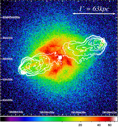
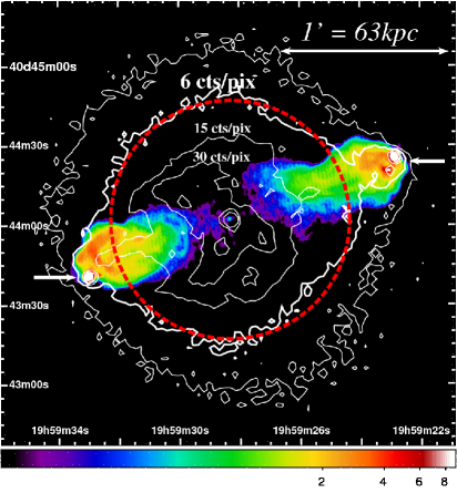
Figure 1.— $\it Left$: The co-added raw 0.7–7 keV ACIS image of Cygnus A. Color scale of the image shows the photon counts for each pixel; scale bar is shown below. White contours represent the radio strength of the 1.3 GHz band observed by the VLA, the contours levels are 0.053, 0.2, 0.8, 1.2, 2, 5 and 10 $\rm Jy~{}beam^{-1}$ for a beam size of 1.19$\arcmin$$\times$1.12$\arcsec$. $\it Right$: ACIS contours image of Cygnus A at 0.7–7 keV, superposed on the 1.3 GHz VLA image of the $\rm Jy~{}beam^{-1}$ for each pixel; scale bar is shown below. Five contours represent X-ray brightness of 3, 6, 15, 30, 50 and 100 counts per pixel.

Due to the faintness of the IC X-rays emitted from the lobes, the objects located at the edge of the cluster of galaxies have been targeted, owing to the poor radiation from the intra-cluster medium (ICM). In the past 20 years, around 30 objects have been observed with $ASCA$ and $ROSAT$ (e.g., Kaneda et al. 1995; Feigelson et al. 1995; Tashiro et al. 1998, 2001), as well as with the $\it Chandra~{}X$-$\it ray~{}observatory$, $\it XMM$-$\it Newton$ and $\it Suzaku$ (e.g., Burunetti et al. 2001; Isobe et al. 2002, 2005; Hardcastle et al. 2002; Grandi et al. 2003; Comastri et al. 2003; Croston et al. 2004; Kataoka & Stawarz 2005; Tashiro et al. 2009). In most cases, the seed photons were determined to be CMB photons. The measured IC X-ray flux from the lobes often requires that $u_{\rm e}$ is considerably greater than $u_{\rm m}$ (e.g., Tashiro et al. 1998; Isobe et al. 2002), as well as that the magnetic field ($B_{\rm IC}$) is smaller than the magnetic field estimated under equipartition ($B_{\rm eq}$), $B_{\rm IC}/B_{\rm eq}=0.1$–1 (e.g., Croston et al. 2005). Against this background, it is of great interest to investigate the energy balance between the relativistic electrons and the magnetic fields under ICM pressure in order to argue the energetics from the nuclei to inter-galactic space.

In this paper, we present an examination of the diffuse lobe emission from one of the brightest radio lobe objects surrounded by ICM, Cygnus A. Cygnus A is a well-known FR II (Fanaroff & Riley 1974) radio galaxy with an elliptical host. The radio images show symmetrical double-lobe morphology with an extremely high radio flux density $S_{\rm SR}=1598$ Jy at 1.3 GHz (Bîrzan et al. 2004), which makes it the brightest radio galaxy in the observable sky. Measuring radio fluxes between 151 MHz and 5000 MHz, Carilli et al. (1991) found spectral breaks whose break frequencies vary with position on the lobes. The spectral energy index below and above the break is 0.7 and 2, respectively. X-ray observations show diffuse X-ray emission, which is considered to originate from ICM (e.g., Smith et al. 2002), as well as a cavity corresponding to the radio lobe (e.g., Wilson et al. 2006). In addition to the thermal emissions, we examined non-thermal X-ray emissions from the lobes of Cygnus A utilizing the excellent spatial resolution of Chandra.

The structure of this paper is as follows. We describe the archived $\it Chandra$ observation data on Cygnus A and the results of careful X-ray analysis in $\S~{}2$ and $\S~{}3$. Following the presentation of the results, namely, the suggestion of non-thermal X-ray emissions from the lobes, we report the spectral energy distribution of the Cygnus A lobes, as determined from radio and X-ray data, and estimate the emission of seed photons and the physical parameters of the lobes in $\S~{}4$. Finally, we summarize these results in the last section. Throughout this paper, we adopt a cosmology with $H_{0}=71$ km s^-1 Mpc^-1, $\Omega_{\rm M}=0.27$ and $\Omega_{\Lambda}=0.73$ (Komatsu et al. 2009), where $1\arcmin$ corresponds to 63 kpc at the red shift $\it z$=0.0562 (Stockton et al. 1994) of Cygnus A.

2. X-ray observation and data reduction

Cygnus A has been observed with the Advanced CCD Imaging Spectrometer (ACIS) detector on the $\it Chandra~{}X$-$Ray~{}Observatory$ on nine occasions in the full frame mode. Seven out of nine the observations were performed with ACIS-I1 front-illuminated (FI) CCDs, one with ACIS-I3 FI CCDs and the rest with ACIS-S3 back-illuminated (BI) CCDs. The total exposure of ACIS-I1, ACIS-S3 and ACIS-I3 is 172.2 ks, 34.7 ks and 29.7 ks, respectively. Table 1 summarizes the nine ACIS observations of Cygnus A. These observations were performed with the default frame time of 3.2 s using the FAINT (ACIS-S3) and VFAINT (ACIS-I1 and I3) format.

Table 1Observation log of $Chandra$/ACIS

OBS-ID		Instrument	Date	Exposure (ks)
0360		ACIS-S3	2000.05.21	34.7
6225		ACIS-I1	2005.02.15	25.8
5831		ACIS-I1	2005.02.16	51.1
6226		ACIS-I1	2005.02.19	25.4
6250		ACIS-I1	2005.02.21	7.0
5830		ACIS-I1	2005.02.22	23.5
6229		ACIS-I1	2005.02.23	23.4
6228		ACIS-I1	2005.02.25	16.0
6252		ACIS-I3	2005.09.07	29.7
total		–	–	172.2

The data were reduced using the CIAO version 4.1 software package, and we performed the data analysis using HEASOFT version 6.8. We reprocessed all the data by following standard procedures in order to create new “level-2” event files by utilizing CALDB version 4.1.2. We applied the latest gain and charge transfer inefficiency corrections and a new bad pixel file created with acis_run_hotpix. We generated a clean data set by selecting standard grades (0, 2, 3, 4 and 6). After removing the point X-ray sources within the field of view of ACIS and the Cygnus A region, we produced a light curve covering the entire CCD chip. Using lc_sigma_chip, we excluded high background time regions whose threshold was more than 3 $\sigma$ above the mean.

Thus, we obtained good exposure of 167.6 ks for ACIS-I1, 29.7 ks for ACIS-I3 and 34.5 ks for ACIS-S3.

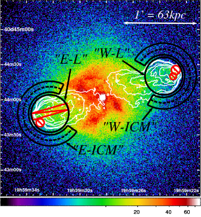
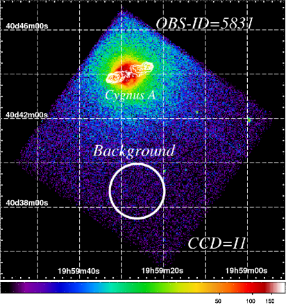
Figure 2.— $\it Left$: ACIS X-ray image in the 0.7–7 keV range. The 1.3 GHz VLA contour is overplotted. The integration region for spectral analysis is shown. The areas enclosed by black solid-line circles are the “lobe regions”. The red solid-line circle and rectangle represent excluded hotspots and jet regions. The areas enclosed by solid-line concentric annuli are the regions surrounding the lobes (see text). $\it Right$: Raw ACIS–I1 data of obsid=5831 X–ray image, binned into $4\times 4$ ACIS pixels. The 1.3 GHz VLA contour is overplotted. The area enclosed by the solid-line circle denotes the background region.

3. Results of X-ray analysis

3.1. X-ray image and selection of integration region

The left panel of Fig. 1 shows the 0.7–7 keV $\it Chandra$ image composed of nine co-added data sets with merge_all from CIAO in gray scale, on which 1.3 GHz radio contours are overplotted. Details of the radio data are given in § 4. The AGN nucleus is observed at $\alpha(2000)=19^{h}59^{m}28.3^{s}$, $\delta(2000)=+40\arcdeg 44\arcmin 02\arcsec$. The hotspots are located in the eastern and western lobe. The distance between the two hotspots is $\sim 120\arcsec$, which corresponds to the projected distance of about 126 kpc. The western lobe is approaching and the eastern lobe is receding from us (Perley et al. 1984). X-ray emission that extends to the vicinity of the nucleus is explained by Smith et al. (2002) as the ICM of $\it kT\sim$ 4–9 keV. The right panel of Fig. 1 shows the 1.3 GHz VLA image in gray scale on which X-ray brightness contours (solid line) are overplotted. From the X-ray contours of 15 counts per pixel, faint X-ray emission can be seen from the jet located to the east of the nucleus ($\alpha(2000)=19^{h}59^{m}31.0^{s}$, $\delta(2000)=+40\arcdeg 43\arcmin 52\arcsec$), and the eastern hotspot (Steenbrugge et al. 2008). It appears that the X-ray contours at 15 counts per pixel (thin line) form a “cavity” in the ICM avoiding the 1.3 GHz lobe. On the other hand, beyond the dashed circle at $45\arcsec$ from the nucleus, the contours at 6 counts per pixel (thick line) show an extended structure in the direction of the 1.3 GHz lobe on the east and west sides (arrows in the right panel of Fig. 1). These extended structures are apparently associated with the lobes, although the X-rays from the lobes are thought to be contaminated with X-rays from the foreground and background ICM.

In order to evaluate the extended emission along the lobes, we accumulated the X-ray spectra from the regions shown in Fig. 2 ($\it left$). The regions “Eastern–Lobe” (“E–L”) and “Western–Lobe” (“W–L”) are marked with circles with a radius of $16\arcsec$ (16.8 kpc), corresponding to the 1.3 GHz contours. However, in order to avoid X-ray emissions from hotspots and jets (Steenbrugge et al. 2008), we excluded hotspots and jet regions. Moreover, to investigate the ICM in the foreground and background of the lobes, we accumulated X-ray spectra from the ICM surrounding the lobes. We set concentric annuli around the lobe, with inner and outer radii of 18.2$\arcsec$ and 27.6$\arcsec$, respectively, which are denoted as “Eastern–ICM” (“E–ICM”) and “Western–ICM” (“W–ICM”), as shown in Fig. 2 ($\it left$). The region facing the nucleus is excluded so as to avoid contamination from the lobes and jets.

The background spectrum is estimated in another circular region, avoiding bright ICM emission as well as point sources. The background spectra are accumulated from the same circular region whose radius is 74$\arcsec$ (77.7 kpc) and the center is placed at ($\alpha(2000)=19^{h}59^{m}29.2^{s}$, $\delta(2000)=+40\arcdeg 38\arcmin 29\arcsec$) for the ACIS-I1 and ACIS-S3. Because of the different roll angle at the ACIS-I3 observation, we cannot choose the same region for the background, but had to set the center at ($\alpha(2000)=19^{h}59^{m}52.3^{s}$, $\delta(2000)=+40\arcdeg 46\arcmin 38\arcsec$) with a radius same to the background of the ACIS-I1 and ACIS-S3. Although the two regions may contain different unresolved sources, we confirmed there is no difference in the obtained background spectra In Fig. 2 ($\it right$), the background region of obsid=5831 is shown as an example.

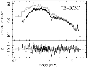
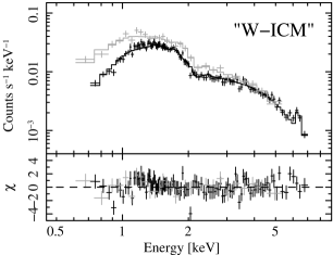
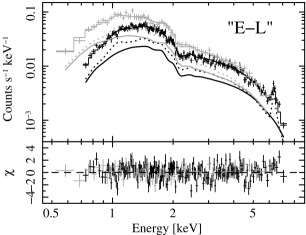
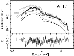
Figure 3.— $\it top$: Background-subtracted 0.7–7 keV ACIS-FI (black) and 0.5–6 keV ACIS-BI (gray) spectra of the regions surrounding the eastern (left) and western (right) lobes. Histogram is a best-fit Mekal model spectrum absorbed by galactic $N_{\rm H}$. The lower panel shows the residuals of the absorbed Mekal model fit. $\it bottom$: Background-subtracted 0.7–7 keV ACIS-FI (black) and 0.5–6 keV ACIS-BI (gray) spectra of the eastern (left) and western (right) lobes. The histogram with the solid line is a best-fit (PL+Mekal) model. The included PL and Mekal components are indicated by solid and dotted lines. Both model spectra are modified by galactic absorption. Lower panel shows the residuals of the absorbed (Mekal+PL) model.

3.2. X-ray spectrum of ICM surrounding the lobe

We first investigated the possible temperature gradient of the ICM in the “E–ICM” and “W–ICM” regions. For that purpose, we divided each region in two, as shown by the dashed lines in Figure 2 ($\it left$): the inner regions are “E–ICM1” and “W–ICM1”, and the outer regions are “E–ICM2” and “W–ICM2”. Spectra were extracted from all of nine data sets using specextract from CIAO. We added the spectra acquired with FI CCDs (ACIS-I1 and ACIS-I3) using mathpha from FTOOL and performed joint fitting with the spectrum acquired with BI CCDs (ACIS-S3). In the following, these spectra are referred to as ACIS-FI (ACIS-I1 and ACIS-I3) and ACIS-BI (ACIS-S3). Furthermore, we introduced a constant factor for the relative normalization of ACIS-FI and ACIS-BI. Then, we introduce a single-temperature Mekal model (Mewe et al. 1995) to estimate the ICM component absorbed by Galactic $N_{\rm H}$ (fixed at $3.5\times 10^{21}\rm~{}cm^{-2}$; Dickey & Lockman 1990). The solar abundances of Anders & Grevesse (1989) were used throughout. The response matrix files (rmf) and the auxiliary response file (arf) for the model were produced from observation data with specextract from CIAO, and then weighted by their exposure and added with addrmf and addarf from FTOOL. Each energy bin was set to include at least 80 counts ($\sim 9\sigma$/bin). In consideration of the decrease in source photons, the quantum efficiency and the increase in the background that is intrinsic to the detector in high and low energy bands, we selected the more reliable 0.7–7 keV range for ACIS-I and 0.5–6 keV for ACIS-S to maximize the signal-to-noise ratio. The best-fit spectral parameters are listed in Table 2, and we obtained an acceptable fit. The values for the inner and outer regions are in fairly good agreement. Thus, significant $kT$ and $Z/Z_{\odot}$ gradients were not observed in the ICM surrounding the lobe within a 90% confidence level. Next, we analyzed “E–ICM” and “W–ICM”. Figure 3 (top) presents the background-subtracted ACIS-I 0.7–7 keV and ACIS-S 0.5–6 keV spectra of the “E–ICM” and “W–ICM” regions. The best-fit spectral parameters are listed in Table 2. We obtained an acceptable fit with $\chi^{2}/dof$=190.13/185 (“E-ICM”) and 135.76/130 (“W-ICM”) ($P(\chi)=0.382$ and $0.347$, respectively). Therefore, we adopted the values of $kT$ and $Z/Z_{\odot}$ derived in this analysis as the spectral parameters for the ICM foreground and background of the lobes.

Table 2 Best-fit spectral parameters of ICM surrounding the Cygnus A lobes

Region	$N_{\rm H}$	$kT$ (keV)	$Z/Z_{\odot}$	Norm	Constant	$\rm\chi^{2}$/dof
E–ICM1	0.35	$5.38^{+0.43}_{-0.42}$	$0.62^{+0.20}_{-0.19}$	$4.06^{+0.25}_{-0.17}$	1.05${}^{+0.07}_{-0.06}$	101.63/91
E–ICM2	0.35	$4.81^{+0.40}_{-0.31}$	$0.65^{+0.19}_{-0.18}$	$4.39^{+0.24}_{-0.23}$	1.10$\pm 0.06$	95.47/98
E–ICM	0.35	$5.11\pm 0.28$	$0.63\pm 0.13$	$8.50^{+0.32}_{-0.31}$	1.08$\pm 0.04$	190.13/185
W–ICM1	0.35	$8.07^{+1.33}_{-1.07}$	$0.49^{+0.33}_{-0.30}$	$2.51\pm 0.17$	1.08$\pm 0.08$	62.75/62
W–ICM2	0.35	$6.87^{+0.85}_{-0.79}$	$0.57^{+0.27}_{-0.24}$	$3.00\pm 0.18$	0.97$\pm 0.07$	73.96/73
W–ICM	0.35	$7.25^{+0.77}_{-0.60}$	$0.48^{+0.18}_{-0.17}$	$5.56\pm 0.23$	1.01${}^{+0.06}_{-0.05}$	135.76/130

Table 3Results for four models fit to the ACIS spectrum of the lobe region

		$kT_{1}$		$kT_{2}$(keV)			Norm2
Region	M	(keV)	$Z_{1}/Z_{\odot}$	Norm1	$\Gamma_{\rm X}$	$Z_{2}/Z_{\odot}$	$S_{1\rm keV}$ (nJy)	Constant	$\chi^{2}$/dof
E-L	(a)	5.11 (fix)	0.63 (fix)	$10.36^{+0.17}_{-0.19}$	–	–	–	1.08$\pm 0.04$	286.03/217
	(b)	$5.84^{+0.36}_{-0.30}$	$0.51^{+0.12}_{-0.11}$	10.48${}^{+0.33}_{-0.32}$	–	–	–	1.09$\pm 0.04$	244.83/215
	(c)	5.11 (fix)	0.63 (fix)	8.33${}^{+0.30}_{-5.63}$	15.32${}^{+\infty}_{-9.20}$	0.63 (fix)	2.01${}^{+5.49}_{-0.91}$	1.09$\pm 0.04$	244.03/215
	(d)	5.11 (fix)	0.63 (fix)	5.84${}^{+1.51}_{-1.54}$	$1.69^{+0.07}_{-0.13}$	–	$77.7^{+28.9}_{-31.9}$	1.08$\pm 0.04$	224.06/215
W-L	(a)	7.25 (fix)	0.48 (fix)	7.92${}^{+0.16}_{-0.15}$	–	–	–	1.03${}^{+0.05}_{-0.04}$	273.18/178
	(b)	6.55${}^{+0.49}_{-0.47}$	0.43$\pm 0.13$	8.08${}^{+0.28}_{-0.27}$	–	–	–	1.03${}^{+0.04}_{-0.05}$	262.83/176
	(c)	7.25 (fix)	0.48 (fix)	7.87${}^{+0.15}_{-0.16}$	0.22${}^{+0.46}_{-0.08}$	0.48 (fix)	0.85${}^{+3.45}_{-0.75}$	1.02${}^{+0.04}_{-0.05}$	255.54/176
	(d)	7.25 (fix)	0.48 (fix)	5.31${}^{+2.49}_{-2.01}$	$1.84^{+2.90}_{-0.12}$	–	$52.4^{+42.9}_{-42.4}$	1.02${}^{+0.04}_{-0.05}$	241.29/176

3.3. X-ray spectrum of lobe region

Figure 3 (bottom left) shows the background-subtracted ACIS-I 0.7–7 keV and ACIS-S 0.5–6 keV spectra from the “E–L” region. Model (a): Firstly, we evaluated the spectrum with a single-temperature Mekal model whose $kT$ and $Z/Z_{\odot}$ were fixed as the values for the ICM surrounding the lobe regions “E–ICM” (§3.2). The obtained value of $\chi^{2}/dof=286.0/217$ ($P(\chi)=0.001$) indicates that the single-temperature model is unacceptable. Model (b): Secondly, we refit the spectrum with the Mekal model whose $kT$ and $Z/Z_{\odot}$ were freed. The best-fit parameters are listed in Table 3. Again, we obtained a unacceptable fit with $\chi^{2}/dof=244.8/215$ ($P(\chi)=0.079$), and the evaluated $kT$ was significant larger than that of the ICM surrounding the lobe. Unlike the “E–ICM” spectrum, the “E–L” spectrum cannot be described with a single-temperature thermal emission model. In order to determine the other X-ray emission mechanism, we estimated the spectrum with additional models. Model (c): We added second Mekal model. The values of $kT$ and $Z/Z_{\odot}$ for one of the two components were fixed as the average values for the ICM surrounding the lobe, in order to represent the ICM in the foreground and background of the lobe, but the values for the second component were freed to fit the spectrum. The best-fit parameters are presented in Table 3, but the resultant value of $\chi^{2}/dof=244.03/215$ ($P(\chi)=0.085$) is not significantly improved. Model (d): Finally, we added a power-law (PL) model instead of the additional Mekal model in (c). The best-fit parameters are shown in Table 3. The improved value of $\chi^{2}/\rm dof=224.06/215$ ($P(\chi)=0.342$) indicates that this fit is acceptable. Figure 3 (bottom left), shows the histogram of the PL+Mekal model (upper panel) and the residual (lower panel). The best-fit photon index and flux density at 1 keV for the PL are $\Gamma$=$(1.69\pm 0.06)^{+0.03}_{-0.12}$ and $S_{\rm 1keV}$=$(77.7^{+28.3}_{-28.7})^{+6.0}_{-14.0}~{}\rm nJy$, respectively. The first error for each parameter indicates the 90% confidence level including the error arising from normalization of the Mekal model and the systematic error between ACIS-FI and ACIS-BI. The second error indicates the systematic error at the 90% confidence level for both $kT$ and $Z/Z_{\odot}$ from the evaluation of the “E–ICM” spectrum (§3.2). The resultant errors are shown in Table 3, and the PL flux is not a 3-$\sigma$ detection. As an interpretation of non-thermal emission, the PL model naturally implies a lobe source.

The derived high temperature for the second Mekal component in Model (c) possibly suggests shock-heating in the ICM or additional high-temperature plasma in the lobe. Although a shock-heated shell has been detected in Cygnus A (Wilson et al. 2006), the shock-heated shell region is not included in the spectrum-integrated regions in the present study. Furthermore, the derived thermal electron density of $(1.37^{+2.42}_{-0.99})\times 10^{-2}~{}\rm cm^{-3}$ of the eastern lobe, where we assumed that thermal plasma volume is a sphere of radius 16.8 kpc in the integrated region, is larger by nearly two orders of magnitude than the thermal electron density of $<10^{-4}~{}\rm cm^{-3}$ reported by Dreher et al. (1987) and Carilli et al. (1998), based on their radio rotation measurements from the region. However, this limit can be two orders of magnitude larger assuming a tangled magnetic field. Therefore, the thermal interpretation is still a possibility.

Figure 3 (the bottom right) shows the background-subtracted ACIS-I 0.7–7 keV and ACIS-S 0.5–6 keV spectra from the “W–L” region. Moreover, in Table 3, each best-fit parameter is listed for the spectra in the “W–L” region, which is evaluated in the same manner as the “E–L” region. Although the X-ray brightness of the “W–L” region is half that of the “E–L” region and the temperature of the ICM surrounding the western lobe is fairly high, the improvement is not clear. Among the four models, Model (d) provides the best result, $\chi^{2}/\rm dof=241.29/176$ ($P(\chi)=0.01$), as in the case of the “E–L” spectrum. The best-fit photon index and flux density at 1 keV for the PL are $\Gamma$=$(1.84^{+2.86}_{-0.12})^{+0.50}_{-0.04}$ and $S_{\rm 1keV}$=$(52.4^{+42.9}_{-42.4})^{+29.0}_{-0}~{}\rm nJy$, respectively. The flux density at 1 keV of the PL from the western lobe indicates a dimmer non-thermal component than that of the eastern lobe. Although the western lobe is closer to us, the distance between the eastern and western lobes ($\sim$126 kpc) is negligible in comparison with the distance between Earth and Cygnus A ($\sim 250$ Mpc). Furthermore, assuming the hotspot speed to be the upper limit of the expanding speed of the lobes, the effect of beaming can be disregarded since the speed of the hotspot is $\sim 0.01c$ (Carilli et al. 1991).

Therefore, the differences are possibly attributable to intrinsic differences between the individual lobes.

4. Broadband spectra and physical parameters of the lobes

In this section, we estimate the physical parameters of the Cygnus A lobes by comparing the radio and X-ray data with those predicted by one-zone emission models. Radio data analysis for the estimation of lobe flux is presented in $\S~{}4.1$. The comparisons of the observations and models and the obtained physical parameters are presented in $\S~{}4.2$.

4.1. Estimation of radio-lobe flux

We used archived data on Cygnus A at 1.3, 1.7, 4.5, and 5.0 GHz that was acquired by the VLA in various configurations. The A and C VLA configurations were chosen to sample the $u$-$v$ plane adequately on the shortest baselines necessary and to provide good resolution when mapping the detailed source structure. These data are summarized in Table 4 and Table 5. The data were calibrated by using the Astronomical Image Processing System (AIPS) software package developed by the NRAO. 3C 286 was used as a primary flux calibrator. Observations in different VLA configurations were imaged separately by using the CLEAN algorithm and self-calibrated several times. This self-calibration was performed with the Difmap software package (Shepherd et al. 1994). Then, the data sets acquired in different configurations for the same frequency were combined to improve the $u$-$v$ coverage by using the AIPS task DBCON. The combined data sets were used to produce the final images after a number of iterations with CLEAN and self-calibration with Difmap.

Firstly, we convolved the images at all frequencies to obtain the same resolution at 1.3 GHz. Then, we estimated the lobe flux density by integrating the flux density within the circle with the radius of 16$\arcsec$ (hereafter 16$\arcsec$ circle) shown in Figure 4 and subtracting the flux of hotspots from the integrated flux of the 16$\arcsec$ circle. In the X-ray image, one hotspot and two hotspots can be seen in the eastern and western lobes, respectively (Fig. 2). In the radio images, these hotspots can be clearly identified. We characterized the flux of each hotspot by fitting a model of the emission from a two-dimensional elliptical Gaussian. The estimated hotspot and lobe fluxes are presented in Table 6. Following the analysis in X-ray, we do not subtract the overlapping lobe fluxes from the Gaussian fit regions. We neglected the emission from the jet because the jet emission only accounts for $\sim 5\%$ of the lobe flux (Steenbrugge et al. 2010). Neglecting the emission from the jet does not affect the result of spectral energy distribution (SED) fit in $\S~{}4.2$ significantly.

Table 4Properties of VLA data

Date	Array	Frequency	Bandwidth
	configuration	(MHz)	(MHz)
1983 Oct 24	A	4525, 4995	25
1984 Apr 15	C	4525, 4995	25
1986 Dec 1	C	1345, 1704	6.25, 6.25
1987 Aug 18	A	1345, 1704	3.13

Table 5Properties of VLA data

Frequency	Flux	Beam size	P.A.	$\sigma_{r.m.s.}$
(MHz)	(Jy)	(arcsec)	(deg)	(mJy beam-1)
1345	1580.48	1.19 $\times$ 1.12	87.6	17.53
1704	1290.10	0.96 $\times$ 0.91	81.4	11.54
4525	406.58	0.39 $\times$ 0.33	-86.6	0.82
4995	366.08	0.36 $\times$ 0.30	-86.6	0.83

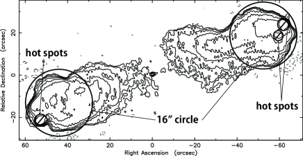
Figure 4.— Image of Cygnus A at 1.3 GHz. Contours are plotted at levels of 3$\sigma$ $\times$ (-1, 1, 2, 4, 8, 16, 32, 64). The r.m.s. noise level is $\sigma$=17.53 mJy/beam. The circle indicates the region where the lobe flux density was estimated.

Table 6Radio lobe / hotspot flux density

Frequency		$I_{\rm tot}\tablenotemark{a}$	${I_{\rm hot}\tablenotemark{b}}$	${I_{\rm lobe}\tablenotemark{c}}$
(MHz)		(Jy)	(Jy)	(Jy)
1345	Eastern lobe	718$\pm 36$	124$\pm 6$	594$\pm 36$
	Western lobe	579$\pm 29$	150$\pm 5$	429$\pm 29$
1704	Eastern lobe	580$\pm 29$	117$\pm 4$	463$\pm 29$
	Western lobe	477$\pm 24$	120$\pm 4$	357$\pm 24$
4525	Eastern Lobe	192$\pm 10$	63$\pm 2$	129$\pm 10$
	Western lobe	175$\pm 9$	53$\pm 2$	122$\pm 9$
4995	Eastern lobe	174 $\pm 9$	59$\pm 2$	115$\pm 9$
	Western lobe	159 $\pm 8$	51$\pm 2$	108$\pm 8$

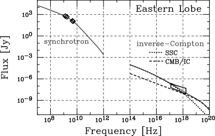
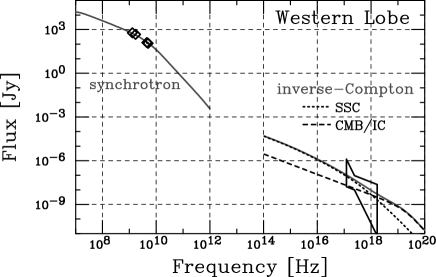
Figure 5.— Spectral energy distribution of the eastern (left) and western (right) lobes of Cygnus A. Areas enclosed by solid lines: X-ray spectrum obtained with $\it Chandra$. Diamonds: integration flux obtained at 1.3 GHz, 1.7 GHz, 4.5 GHz and 5 GHz. Derived models for synchrotron and IC emissions are shown by solid lines at lower and higher frequencies. For the IC emissions, the dashed line represents CMB-boosted IC emission and the dotted line represents SSC emission.

Table 7Physical parameters for lobes of Cygnus A

Parameter		Unit	Eastern lobe	Western lobe
Volume of lobe (V)		$\rm cm^{3}$	5.8 $\times 10^{68}$
Min electron Lorentz factor ($\gamma_{\rm min}$)		–	1
Max electron Lorentz factor ($\gamma_{\rm max}$)		–	$10^{5}$
Normalization of electron energy spectrum ($N_{\rm 0}$)		$\rm cm^{-3}$	3.1$\times 10^{-3}$	1.6$\times 10^{-3}$
Electron break Lorentz factor ($\gamma_{\rm b}$)		–	7$\times 10^{3}$	6$\times 10^{3}$
Magnetic field ($B_{\rm IC}$)		$\mu\rm G$	15	22
Ratio of $B_{\rm IC}$ and $B_{\rm eq}\tablenotemark{a}$  ($B_{\rm IC}/B_{\rm eq}$)		–	0.30	0.44
Magnetic energy density ($u_{\rm m}$)		$\rm erg~{}cm^{-3}$	$9.0\times 10^{-12}$	$2.0\times 10^{-11}$
Electron energy density ($u_{\rm e}$)		$\rm erg~{}cm^{-3}$	$6.0\times 10^{-9}$	$3.2\times 10^{-9}$
Ratio of $u_{\rm e}$ and $u_{\rm m}$ ($u_{\rm e}$/$u_{\rm m}$)		–	666 (35 )	160 (11 )

4.2. Physical parameters of the lobes

Figure 5 shows the X-ray and radio SEDs of the eastern and western lobes of Cygnus A. In the X-ray analysis, the eastern jet region was excluded from the integrated lobe region in a circle with a radius of 16$\arcsec$. In order to match the area fitted in the X-ray analysis to that fitted in the radio analysis, we renormalized the X-ray fluxes by a factor of 1.34 for the eastern lobe. Consequently, it can be clearly seen that the radio spectrum does not connect smoothly to the X-ray spectrum; therefore, diffuse X-rays are produced via the IC process caused by SR electrons in the lobe.

4.3. Physical parameters of the lobes

In order to determine the origin of seed photons boosted to the X-ray range, we estimate the energy density of IR photons ($u_{\rm IR}$), SR photons ($u_{\rm SR}$) and CMB photons ($u_{\rm CMB}$) in the lobe. Here, we adopted $u_{\rm CMB}=4.1\times 10^{-13}(1+z)^{4}~{}\rm erg~{}cm^{-3}$ ( Harris & Grindlay 1979), $u_{\rm IR}=L_{\rm IR}/4\pi cd^{2}~{}\rm erg~{}cm^{-3}$, and assumed IR luminosity of $L_{\rm IR}\sim 10L_{\rm X}\sim 1.8\times 10^{44}~{}\rm erg~{}s^{-1}$, considering the typical spectrum of quasars (Sanders et al. 1989 and Young et al. 2002). $d$ is the distance from the nucleus (e.g., Brunetti et al. 2001), and $u_{\rm SR}=3L_{\rm SR}/4\pi cr^{2}~{}\rm erg~{}cm^{-3}$, where $L_{\rm SR}$ is the SR luminosity and $r$ is the radius of the lobe. $L_{\rm SR}$ was calculated by integrating the flux between 10 MHz and 5 GHz, where we assumed a PL spectrum, $S_{\nu}=S_{\nu_{0}}(\nu/\nu_{0})^{-\alpha}$ with $\alpha$=0.7 (Carilli et al. 1991). We used the 1.3 GHz flux listed in Table 6 for $S_{\nu_{0}}$, and the radius of each lobes was set to 16.8 kpc. Thus we obtained $u_{\rm CMB}\sim 5.6\times 10^{-13}~{}\rm erg~{}cm^{-3}$, $u_{\rm IR}\sim 2.0\times 10^{-13}~{}\rm erg~{}cm^{-3}$ and $u_{\rm SR}\sim 7.0\times 10^{-13}~{}\rm erg~{}cm^{-3}$ , respectively. Therefore, we consider $u_{\rm CMB}$ and $u_{\rm SR}$ to be dominant in the lobe in the following discussion. In order to estimate the $u_{\rm e}$ and $u_{\rm m}$ values that are spatially averaged over the lobes in the “E–L” and “W–L” regions, the X-ray and radio fluxes were evaluated through modeling. We used the SR and synchrotron self-Compton (SSC) model with software developed by Kataoka (2000) and a CMB boosted IC (CMB/IC) component calculated in accordance with Harris & Grindlay (1979). Here, we assume that SR and IC emissions are produced by the same population of relativistic electrons. According to Carilli et al. (1991), the sharp cutoff in the SR radio spectrum indicates a broken power law with an energy index before and after the breaks at 0.7 and 2. We assume the electron distribution is $N_{\rm e}(\gamma)=N_{0}\gamma^{-\rm s_{1}}$ for $\gamma<\gamma_{\rm b}$ and $N_{\rm e}(\gamma)=N_{0}\gamma_{\rm b}^{s_{2}-s_{1}}\gamma^{-\rm s_{2}}$ for $\gamma>\gamma_{\rm b}$, where $N_{0}$ is the normalization of the electron energy spectrum, $\gamma$ is the electron Lorentz factor and $s$ is the electron energy spectrum index. Moreover, $\gamma_{\rm b}$ is the break Lorentz factor. The index of $s_{1}$ and $s_{2}$ is 2.4 and 5 ($s=2\alpha+1$), respectively, and the assumed range of $\gamma_{\rm min}-\gamma_{\rm max}$ is $1-10^{5}$. We fixed the volume parameter to $V$=$4\pi r^{3}/3$=$5.8\times 10^{68}~{}\rm cm^{3}$ of the lobe and assumed a sphere with a radius of $16.8~{}\rm kpc$, which was the same as the radius of the integration circle in the X-ray and radio analyses (§ 3). We tuned the magnetic field $B$, $\gamma_{\rm b}$ and $N_{0}$. From the eastern and western radio spectra, the SR turnover frequency is assumed to be around 1 GHz. Under the above conditions, we evaluated the appropriate SR, SSC and CMB/IC components to reproduce the X-ray and radio fluxes, which are plotted in Fig. 5. The X-ray data is reproduced well by the CMB/IC and SSC emissions. Unlike the emissions from other radio lobes that have been reported to date (§ 1), the SSC component in the emissions from the lobes of Cygnus A contributed significantly to the X-ray band. The SSC component accounts for 80% and 40% of the total IC component at $\sim$0.6 keV and $\sim$ 7 keV, respectively. The SSC X-ray component is produced by electrons with a Lorentz factor of $\sim$$10^{4}$–$10^{5}$, and SR emission in the $\sim$1–$10^{2}$ GHz band is produced. Therefore, it is natural to assume that the same distribution of electrons produces the radio and X-ray emissions. The derived parameters are summarized in Table 7. The ratio $B_{\rm IC}/B_{\rm eq}=0.30$ and $0.44$ for the eastern and western lobes, respectively, are in the range previously reported for other objects, $B_{\rm IC}/B_{\rm eq}=(0.1-1)$ (e.q., Croston et al. 2005). The ratio $u_{\rm e}/u_{\rm m}$ appears to show significant electron dominance in the lobes of Cygnus A. Taking $\gamma_{\rm min}=1000$ in order to make a comparison with other radio galaxies, we obtain $u_{\rm e}/u_{\rm m}=$ 35 and 11 for the eastern and western lobes, respectively. Thus, we found that $u_{\rm e}/u_{\rm m}$ for the lobes of Cygnus A at the center of the cluster is similar to that for other field radio galaxies (§ 1).

5. Summary

Using $\it Chandra$ deep observation data (230 ks) for Cygnus A, we carefully analyzed the X-ray spectra of the lobes and the regions surrounding the lobes. Our findings are as follows.

• In $\it Chandra$ X-ray images, among emissions originating from ICM, we confirmed extended X-ray emission regions corresponding to the eastern and western lobes.

• The X-ray spectra of the lobe regions could not be reproduced by a single Mekal model, and we found that the addition of a PL component was more appropriate than the addition of an additional Mekal component in the statistical analysis. The best-fit photon indices of the eastern and western lobe regions were $1.69^{+0.07}_{-0.13}$ and $1.84^{+2.90}_{-0.12}$, and the flux densities at 1 keV were $77.7^{+28.9}_{-31.9}~{}\rm nJy$ and $52.4^{+42.9}_{-42.4}~{}\rm nJy$, respectively.

• The obtained X-ray and radio SED of the lobes supported the IC mechanism for X-ray emission. Furthermore, the X-rays are likely produced via both SSC processes below $\sim 10^{18}$ Hz (4 keV) and CMB/IC processes above $\sim 10^{18}$ Hz (4 keV). This is the first case of a lobe where SSC emission has been found to affect IC emission.

• The derived physical parameters under the SSC model indicate that the energy density of electrons dominates that of magnetic fields both in the eastern and western lobes, as often reported from other radio lobe objects.

References

- Anders & Grevesse (1989) Anders, E., & Grevesse, N. 1989, Geochim. Cosmochim. Acta, 53, 197
- Bîrzan et al. (2004) Bîrzan, L., Rafferty, D. A., McNamara, B. R., Wise, M. W., & Nulsen, P. E. J. 2004, ApJ, 607, 800
- Brunetti et al. (1997) Brunetti, G., Setti, G., & Comastri, A. 1997, A&A, 325, 898
- Brunetti et al. (2001) Brunetti, G., Cappi, M., Setti, G., Feretti, L., & Harris, D. E. 2001, A&A, 372, 755
- Carilli et al. (1991) Carilli, C. L., Perley, R. A., Dreher, J. W., & Leahy, J. P. 1991, ApJ, 383, 554
- Carilli et al. (1998) Carilli, C. L., Perley, R., Harris, D. E., & Barthel, P. D. 1998, Physics of Plasmas, 5, 1981
- Comastri et al. (2003) Comastri, A., Brunetti, G., Dallacasa, D., Bondi, M., Pedani, M., & Setti, G. 2003, MNRAS, 340, L52
- Croston et al. (2004) Croston, J. H., Birkinshaw, M., Hardcastle, M. J., & Worrall, D. M. 2004, MNRAS, 353, 879
- Croston et al. (2005) Croston, J. H., Hardcastle, M. J., Harris, D. E., Belsole, E., Birkinshaw, M., & Worrall, D. M. 2005, ApJ, 626, 733
- Dickey & Lockman (1990) Dickey, J. M. & Lockman, F. J. 1990, ARA&A, 28, 215
- Dreher et al. (1987) Dreher, J. W., Carilli, C. L., & Perley, R. A. 1987, ApJ, 316, 611
- Fanaroff & Riley (1974) Fanaroff, B. L. & Riley, J. M. 1974, MNRAS, 167, 31P
- Feigelson et al. (1995) Feigelson, E. D., Laurent-Muehleisen, S. A., Kollgaard, R. I., & Fomalont, E. B. 1995, ApJ, 449, L149
- Grandi et al. (2003) Grandi, P., Guainazzi, M., Maraschi, L., Morganti, R., Fusco-Femiano, R., Fiocchi, M., Ballo, L., & Tavecchio, F. 2003, ApJ, 586, 123
- Hardcastle et al. (2002) Hardcastle, M. J., Birkinshaw, M., Cameron, R. A., Harris, D. E., Looney, L. W., & Worrall, D. M. 2002, ApJ, 581, 948
- Harris & Grindlay (1979) Harris, D. E. & Grindlay, J. E. 1979, MNRAS, 188, 25
- Isobe et al. (2002) Isobe, N., Tashiro, M., Makishima, K., Iyomoto, N., Suzuki, M., Murakami, M. M., Mori, M., & Abe, K. 2002, ApJ, 580, L111
- Isobe et al. (2005) Isobe, N., Makishima, K., Tashiro, M., & Hong, S. 2005, ApJ, 632, 781
- Kaneda et al. (1995) Kaneda, H., et al. 1995, ApJ, 453, L13
- (20) Kataoka, J., Ph.D thesis, 2000, Univ. of Tokyo
- Kataoka & Stawarz (2005) Kataoka, J. & Stawarz, Ł. 2005, ApJ, 622, 797
- Komatsu et al. (2009) Komatsu, E., et al. 2009, ApJS, 180, 330
- (23) Mewe, R., Kaastra, J. S., Liedahl, D. A. 1995, Legacy, 6, 16
- Perley et al. (1984) Perley, R. A., Dreher, J. W., & Cowan, J. J. 1984, ApJ, 285, L35
- Sanders et al. (1989) Sanders, D. B., Phinney, E. S., Neugebauer, G., Soifer, B. T., & Matthews, K. 1989, ApJ, 347, 29
- Shepherd et al. (1994) Shepherd M. C., Pearson T. J., & Taylor G. B., 1994, BAAS, 26, 987
- Smith et al. (2002) Smith, D. A., Wilson, A. S., Arnaud, K. A., Terashima, Y., & Young, A. J. 2002, ApJ, 565, 195
- Steenbrugge et al. (2008) Steenbrugge, K. C., Blundell, K. M., & Duffy, P. 2008, MNRAS, 388, 1465
- (29) Steenbrugge K. C., Heywood I., & Blundell K. M., 2010, MNRAS, 401, 67
- Stockton et al. (1994) Stockton, A., Ridgway, S. E., & Lilly, S. J. 1994, AJ, 108, 414
- Tashiro et al. (1998) Tashiro, M., et al. 1998, ApJ, 499, 713
- Tashiro et al. (2001) Tashiro, M., Makishima, K., Iyomoto, N., Isobe, N., & Kaneda, H. 2001, ApJ, 546, L19
- Tashiro et al. (2009) Tashiro, M. S., Isobe, N., Seta, H., Matsuta, K., & Yaji, Y. 2009, PASJ, 61, 327
- Wilson et al. (2006) Wilson, A. S., Smith, D. A., & Young, A. J. 2006, ApJ, 644, L9
- Young et al. (2002) Young, A. J., Wilson, A. S., Terashima, Y., Arnaud, K. A., & Smith, D. A. 2002, ApJ, 564, 176