Self-organized model of cascade spreading

Abstract

We study simultaneous price drops of real stocks and show that for high drop thresholds they follow a power-law distribution. To reproduce these collective downturns, we propose a minimal self-organized model of cascade spreading based on a probabilistic response of the system elements to stress conditions. This model is solvable using the theory of branching processes and the mean-field approximation. For a wide range of parameters, the system is in a critical state and displays a power-law cascade-size distribution similar to the empirically observed one. We further generalize the model to reproduce volatility clustering and other observed properties of real stocks.

1 Introduction

Cascade spreading is an important emergent property of various complex systems. Real life examples of cascades are numerous and range from infrastructure failures and epidemics to traffic jams and cultural fads Glad00 ; DCLN07 . Theoretical models of cascades usually assume that agents can be in one of two states (healthy or failed) and an agent’s failure puts some stress on its neighbors which may consequently fail too. See LoBaSch09 for a recent survey of this field offering a novel unifying view.

In this paper we focus on cascades in economic systems which can be identified with stock prices suddenly dropping in a major market crash Sorn03 or with companies going bankrupt simultaneously and leading to global recession HoLeLe07 . Theoretical models of such cascades are based on shortage and bankruptcy propagation in production networks WeBa07 , default propagation in credit networks IoJa01 ; SiHo09 , interaction of firms through one monopolistic bank IAFIS09 or in a complex credit network economy DGGRS09 , and herding behavior of traders BaPaSh97 ; CoBo00 . While these models help us to understand cascade processes in economic systems, they are mostly too involved to allow for analytical solutions—their study hence relies on numeric simulations and agent-based modeling MiPa07 .

A simpler point of view on cascade phenomena is offered by the concept of self-organized criticality (SOC) which has had a deep impact on the science of complexity. First introduced more than twenty years ago to explain the ubiquitous $1/f$ noise BTW87 , it caused a blossoming of toy models, computer simulations, and real life experiments Turc99 . The analytical techniques employed include scaling arguments TaBa88 , mean-field theories FlySneBa93 , branching processes Als88 , renormalization methods PiVeZa94 ; Mars94 , and rigorous algebraical techniques Dhar90 .

SOC is a mechanism which explains the emergence of complex behavior in many diverse real world systems PaBa99 ; Sorn06 . The generic behavior of SOC models is: (a) they evolve so that they always stay close to the critical point, (b) long periods of robustness and moderate activity are interrupted by sudden breakdowns. This qualitatively resembles “stock markets which expand and grow on relatively long time scales but contract in stock-market crashes on relatively short time scales” Turc99 and “stock crashes caused by the slow buildup of long-range correlation leading to a global cooperative behavior of the market eventually ending into a collapse in a short time interval” Sorn03 . This similarity provides the main motivation for the present study.

We begin our work with an empirical investigation of simultaneous price drops of real stocks and show that the size distribution of observed events is broad (for high drop thresholds it follows a power-law distribution). This observation suggests that simultaneous stock downturns are a collective phenomenon. We propose a simple dynamical model which for a wide range of parameters self-organizes into a critical state. Unlike most SOC models, our model assumes a probabilistic response mechanism where a node has only a certain probability of reacting to the current stress conditions. The basic idea behind modeling simultaneous stock downturns with cascades is that decline of a single stock may provoke investors’ reactions which consequently may cause other stocks to decline and a “cascade” to spread. The key premise is that while failed nodes become significantly more resistant in the next time step, healthy nodes become slightly less resistant. This close parallel with the slow growth/fast decay picture described above is further supported by our analysis of empirical data which shows that majority of stocks behave in this way. While there are certainly many other effects contributing to the dynamics of market crashes (external shocks, for example), we show that failure propagation alone can reproduce some of the observed patterns.

The minimal model proposed here has the advantage of being simple, not relying on fine-tuning of parameters, analytically solvable in some cases, and easily generalizable to more complicated settings. We analyze it using the formalism of branching processes, the mean-field approximation and, for complex topologies of nodes’ interactions, using numerical simulations. Obtained cascade-size distributions exhibit a close similarity to our empirical observations. Introduction of memory within the model allows us to reproduce other empirically observed features, such as volatility clustering, though at the cost of analytical tractability. We conclude our study with a discussion of further model’s generalizations and possible areas of application.

2 Empirical data

Here we investigate co-occurring price movements of real stocks. Adopting the vocabulary of cascade models, we say that a stock fails when the relative loss of its price over a given time interval $\Delta t$ exceeds a certain threshold $H$. Denoting the price of stock $i$ at time $t$ as $p_{i}(t)$, its failure occurs when $[p_{i}(t)-p_{i}(t+\Delta t)]/p_{i}(t)>H$. The number of stocks failing at time $t$, $n_{F}(t)$, is a direct analog of the cascade size in a model of cascade spreading. As the input data we use daily closing prices (hence $\Delta t=1\,\mathrm{day}$) of 500 stocks from the standard U.S. index S&P 500 (this data is freely available at, for example, finance.yahoo.com). To achieve a fixed system size, we consider only those 332 companies which are in the stock market since the beginning of 1992 and use their prices during the 18-years long period ending in May 2010 for our analysis.

The empirical distribution of failure sizes is shown in Fig. 1 for $H=0\%$ and $H=10\%$. We see that for the large value of $H$ (which is in line with the notion of stock failures), the observed size distribution has a power-law shape. Using the methodology described in ClaShaNew09 , we obtained the power-law exponent $2.19\pm 0.05$ with the lower bound for the power-law behavior $n_{\min}=3$. The corresponding $p$-value (obtained using the standard Kolmogorov-Smirnov statistic) is 0.92 which confirms that the data is consistent with the hypothesis of a power-law distribution. Similar results are obtained also for other threshold values so long as $H\gtrsim 8\%$. When $H\lesssim 8\%$, the resulting size distributions are broad but probably not power-law. Finally, when $H=0\%$ (i.e., any price drop is interpreted as a failure), the size distribution is roughly symmetric around the value corresponding to one half of the system size (see Fig. 1). In the following analysis of empirical data we use the threshold $H=10\%$.

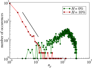
Figure 1: The empirical failure size distribution observed with real stock prices (daily closing prices of 332 companies from January 1992 until May 2010) for threshold relative drops $H=0\%$ and $H=10\%$. The straight line corresponds to the exponent $2.19$ obtained by statistical analysis of the data.

The power-law shape itself suggests that the observed simultaneous stock downturns are rather a collective phenomenon than independent events. This hypothesis is further supported by the average correlation of simultaneously failing stocks, $0.35$ (again including only events with at least three simultaneously failing stocks), which is significantly higher than the overall average stock correlation, $0.25$. Another sign of a strong connection among simultaneously failing stocks comes from their division to ten different industrial sectors according to the GICS classification. The effective number of sectors participating in a cascade is defined as

$$e:=\bigg{(}\sum_{i=1}^{10}r_{i}^{2}\bigg{)}^{-1}$$ (1)

where $r_{i}$ is the relative share of sector $i$ in the cascade and $\sum_{i=1}^{10}r_{i}=1$. By averaging this quantity over all cascades of a given size $S$, we obtain $e(S)$. This number can be compared with the effective number of sectors corresponding to selecting failed stocks at random, $e^{\prime}(S)$. The analysis of stock prices shows that for any $S>3$, $e(S)$ is significantly smaller than $e^{\prime}(S)$ which implies that simultaneous stock failures preferentially affect strongly connected stocks in one sector or in a small number of sectors.

Now we turn our attention to time correlations of failures. The autocorrelation of the number of failing stocks with the time lag one day, $C(n_{F}(t),n_{F}(t+1))\approx 0.15$, is comparable with the autocorrelation of absolute returns, $C(|r(t)|,|r(t+1)|)\approx 0.25$ (the latter result agrees with previous studies Akg89 ; ManSta99 ). The positive autocorrelation values are signs of volatility clustering which is commonly observed in financial data Cont07 . (Loosely speaking, volatility clustering means that large changes tend to be followed by large changes and small changes tend to be followed by small changes, as first noted by Mandelbrot Mand63 .)

We further estimate conditional failure probabilities for individual stocks. For example, $P(F|N)$ denotes failure probability of a stock given that this stock didn’t fail in the previous time step (other three quantities, $P(N|F)$, $P(F|F)$, and $P(N|N)$, follow the same logic). When the results are averaged over all stocks, we obtain $P(F|F)=0.039$ which is much higher than the overall failure probability $P(F)=0.003$—this is another sign of volatility clustering in our data. On the level of individual stocks, however, $62\%$ of all stocks with at least three failures strongly satisfy the inequality $P(N|F)>P(N)$ which is equivalent to $P(F|F)<P(F)$ (because $P(F|F)+P(N|F)=1$). (By strong satisfying we mean that the difference of the two probabilities is greater than the sum of their uncertainties.) We see that despite volatility clustering in the data, most stocks are more “resistant” to failures after they have just undergone one. For the remaining stocks, probabilities $P(N|F)$ and $P(N)$ either differ less than the sum of values’ uncertainties (for $14\%$ of stocks) or even strongly satisfy the opposite inequality $P(N|F)<P(N)$, with corresponding values of $P(F|F)$ often as high as $0.30$ ($24\%$ of stocks).

To summarize, after a failure (a major price drop), most stocks become more resistant to another failure—this observation will serve as a basis for the mathematical model presented in the following section. At the same time, there is a fraction of stocks which are prone to consecutive failures—this particular feature will be discussed in detail in Section 4.

3 Basic model and its mean-field solution

In this section we present a basic model which is amenable to analytical treatment and qualitatively reproduces some of the features observed in empirical data. In its original formulation, this model is particularly suitable for stocks that, as discussed in the previous section, after a failure become more robust. A generalization of the model aiming at reproducing other observed features (volatility clustering, for example) is presented in Section 4.

Consider a system of $N$ nodes where node $i$ ($i=1,\dots,N$) has only two possible states: failed ($i\in\mathcal{F}$) and healthy ($i\not\in\mathcal{F}$). With each node $i$ we further associate fragility $f_{i}\in[0,1]$ which measures how this node reacts to failures of its neighbors (the higher the fragility, the more likely is the node to follow a neighbor’s failure). The dynamics of the model is governed by the following simple rules. (i) In each time step, the first failed node (“trigger”) is chosen at random and may induce failures of other nodes. (ii) If a neighbor of node $i$ fails, node $i$ follows it with probability $f_{i}$ and resists with probability $1-f_{i}$. (If several neighbors of node $i$ fail simultaneously, in order to stay healthy, node $i$ has to resist each individual failure.) The cascade of failures propagates until all remaining nodes resist the damage. (iii) At the end of the time step, fragilities of all nodes are updated according to

$$f_{i}(t+1)=\Big{\{}\begin{aligned} \lambda f_{i}(t)&\qquad i\in\mathcal{F}\\ (1+\beta)f_{i}(t)&\qquad i\not\in\mathcal{F}\end{aligned}$$ (2)

where $0<\beta\ll 1$ and $\lambda\in(0,1)$ are parameters of the model (in effect, failed nodes become less fragile and healthy nodes become slightly more fragile in the next time step). All values $f_{i}(t+1)>1$ are truncated to $1$ (this may occur when $\beta$ is large). After this update is finished, all nodes are again marked as healthy, the current time step ends and a new one begins with point (i). Note that unlike some other models of cascade spreading, failed nodes are not removed from the system in our case. If a long enough equilibration period is applied before measuring the system behavior, the initial fragility values $f_{i}(0)$ are of little importance (see Section 3.5 for a detailed discussion). Unless stated otherwise, we set them randomly in the range $(0,1)$ in our simulations.

According to the rules above, when $n$ neighbors of node $i$ fail, node $i$ resists with the probability $(1-f_{i})^{n}$ and fails with the complementary probability

$$P_{F}(f_{i},n)=1-(1-f_{i})^{n}.$$ (3)

This response to failures is “path-independent” in some sense: the probability that a node resists $n$ failures of its neighbors, $(1-f_{i})^{n}$, is the same as the probability of resisting two consequent waves of failures of $x$ and $n-x$ neighboring nodes, $(1-f_{i})^{x}(1-f_{i})^{n-x}$.

We simplify the system by assuming that interactions of all nodes are equally strong (the general case will be studied in Section 3.4). This renders the notion of “node’s neighbors” superfluous because every failure affects all remaining healthy nodes in the system. Now assume that after the initial failed node is chosen, $n_{1}$ nodes respond to this failure and fail too. Each of the remaining $N-n_{0}-n_{1}$ nodes (here $n_{0}=1$ is the initial number of failed nodes) then has some $n_{1}$-dependent failure probability which results in $n_{2}$ new failures, and so on, until in iteration $m$, $n_{m}=0$ is achieved. The cascade size is then defined as the total number of failures, $S=n_{0}+\dots+n_{m}$, and node fragilities are consequently updated according to Eq. (2). Since in one turn nodes can only fail once, cascade sizes are limited by the system size and $S\leq N$.

The dynamics of the system, based on failure propagation and fragility updating, is fully contained in the three above-described rules. In the following paragraphs we shall study when these rules drive the system to a critical state and what is the distribution of cascade sizes $P(S)$.

3.1 Failure probability

Let $P_{F}$ be the average failure probability of a given node in one time step (or, equivalently, the average fraction of failed nodes in one time step). Assuming that $t_{\mathrm{eq}}$ is some sufficiently long equilibration time (we use $t_{\mathrm{eq}}=10^{4}$ for all our simulations), later fragility values averaged over realizations, $\langle f_{i}\rangle$, do not evolve anymore. All nodes interact equally strongly, hence $\langle f_{i}\rangle$ is independent of $i$ and it can be replaced with $\langle f\rangle$. Since in a large number of time steps $T$ each node undergoes $P_{F}T$ failures and $(1-P_{F})T$ non-failures, Eq. (2) implies

$$\langle f(t_{\mathrm{eq}}+T)\rangle=\langle f(t_{\mathrm{eq}})\rangle\lambda^{P_{F}T}(1+\beta)^{(1-P_{F})T}.$$ (4)

Using the equilibrium condition $\langle f(t_{\mathrm{eq}}+T)\rangle=\langle f(t_{\mathrm{eq}})\rangle$, we can solve this equation with respect to $P_{F}$ to get

$$P_{F}(\beta,\lambda)=-\frac{\ln(1+\beta)}{\ln\frac{\lambda}{1+\beta}}.$$ (5)

When $\beta\ll 1$, this can be approximated with $P_{F}(\beta,\lambda)\approx-\beta/\ln\lambda$ (Fig. 2 compares these results with numerical simulations).

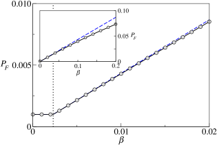
Figure 2: Average failure probability: $P_{F}$ given by Eq. (5) (solid black line), $P_{F}\approx-\beta/\ln\lambda$ (dashed blue line) and numerical results (symbols, averaged over $10^{6}$ time steps) for $N=10^{3}$, $\lambda=0.1$. The vertical dotted line indicates $\beta_{0}$ given by Eq. (6).

A node may fail because it is selected as the first failed node (with probability $1/N$) or due to failure propagation (with probability $P_{P}$); $P_{F}$ thus can be written as $P_{F}=1/N+P_{P}$. Since the value of $P_{F}$ depends solely on $\beta$ and $\lambda$, $P_{P}=P_{F}-1/N$ may be negative for a small system which is, of course, impossible in practice. This situation occurs when for given $\lambda,N$, the value of $\beta$ is smaller than a certain threshold $\beta_{0}$ and hence it does not suffice to compensate for the fragility decay due to $\lambda$. Eq. (4) then has only the trivial solution $\langle f\rangle=0$ and hence $P_{F}(\beta,\lambda)=1/N$ (failures do not spread). When $\beta$ is small, the approximate form of $P_{F}$ can be used to solve this equation with respect to $\beta$ and we get

$$\beta_{0}\approx-\frac{\ln\lambda}{N}$$ (6)

which agrees with numerical simulations (see the vertical line in Fig. 2). Note that if the number of initial failed nodes is assumed to grow with the system size as $wN$ ($w\ll 1$), we get $\beta_{0}\approx-w\ln\lambda$ which is independent of $N$.

When model parameters are set to extreme values (for example, $N=10^{3}$, $\beta=10^{3}$, $\lambda=10^{-3}$), the system exhibits unusual modes of behavior where active turns (with nearly all nodes failed) alternate with calm turns (with nearly all nodes healthy). While Eq. (5) holds also in such conditions, our further analysis focuses on $\beta\ll 1$ which renders more realistic behavior.

3.2 Average fragility

When $nf_{i}\ll 1$, $P_{F}$ given by Eq. (3) can be approximated as $P_{F}(f_{i},n)\approx nf_{i}$ which can be interpreted as independence of stress inflicted by $n$ individual failed nodes. This further means that each failed node has its failing descendants independently of other failed nodes and hence one can use the theory of branching processes Feller70 to describe the cascade spreading. Note that by use of this theory we implicitly assume that the system size is infinite. For a discussion of the finite-size effects on the size of an epidemic outbreak see NaKr04 .

As already mentioned, when interactions of all nodes are equal, $\langle f_{i}\rangle$ is independent of $i$. If we further neglect fluctuations of $f_{i}$, then all nodes have identical fragility $\langle f\rangle$. This is a mean-field-like approximation which replaces the exact cascade spreading with cascade spreading in a homogeneous averaged medium. Since the number of direct descendants now follows a simple binomial distribution with mean $N\langle f\rangle$, we can use elementary results of branching process theory to express the average cascade size (the total progeny) as $\langle S\rangle=1/(1-N\langle f\rangle)$. Further, using $\langle S\rangle=NP_{F}(\beta,\lambda)$ we obtain the average fragility

$$\langle f\rangle=\frac{1}{N}\bigg{(}1-\frac{\ln\big{[}(1+\beta)/\lambda\big{]}}{N\ln(1+\beta)}\bigg{)}.$$ (7)

Since $\beta>0$ and $\lambda<1$, $\langle f\rangle$ is always less than $1/N$. Comparison with numerical simulations (not shown) confirms that Eq. (7) is valid only for $\beta\ll 1$.

3.3 Cascade size distribution

The theory of branching processes is well studied Har89 and can be easily applied to our model. According to a theorem from Dwass69 , if the generating function for the number of direct descendants $d$ is $\pi(x)$, the total progeny of the resulting branching process $Y$ has the distribution

$$P(Y|n_{0})=\frac{n_{0}}{Y}\,p_{Y-n_{0}}^{(Y)}$$ (8)

where $p_{a}^{(b)}$ is defined using

$$[\pi(x)]^{b}=p_{0}^{(b)}+p_{1}^{(b)}x+\dots$$ (9)

and $n_{0}$ is the number of ancestors (in our case, the number of initial failed nodes). Since $d$ obeys a binomial distribution, its generating function is $\pi(x)=(1-\langle f\rangle+\langle f\rangle x)^{N}$ and we get

$$P(S|\beta,\lambda)=\frac{1}{S}\binom{NS}{S-1}\langle f\rangle^{S-1}\big{(}1-\langle f\rangle\big{)}^{NS-S+1}$$ (10)

where we used $n_{0}=1$ and $\langle f\rangle$ is given by Eq. (7). Note that the resulting probability is positive for $S>N$ which contradicts the model assumptions (each node fails at most once in a given turn). This is a direct consequence of using the theory of branching processes which assumes that the system size is infinite. This problem is of little importance for small values of $\beta$ when the obtained values of $P(S)$ are negligible for $S>N$.

When $1\ll S\ll N$, Eq. (10) can be approximated with

$$P(S|\beta,\lambda)=\frac{(N\langle f\rangle)^{S-1}\mathrm{e}^{S(1-N\langle f\rangle)}}{\sqrt{2\pi}S^{3/2}}.$$ (11)

According to Eq. (7), $\lim_{N\to\infty}N\langle f\rangle=1$ for any given $\beta,\lambda$ and hence in the limit of large system size is $P(S|\beta,\lambda)\sim S^{-3/2}$ which corresponds to the classical critical branching process. For a finite system, the smaller the value of $\beta$, the larger the value of $1-N\langle f\rangle$. Consequently, the power-law scaling holds only for $S\ll\beta N$ (this agrees with Fig. 3 where for $\beta=10^{-3}$, the power-law behavior disappears at $S\approx 10$). On the other hand, the range of $\beta$ and $\lambda$ for which the system self-organizes to a critical state is wide and we can say that this is an SOC system.

A comparison of the obtained analytical results with numerical simulations is shown in Fig. 3. The agreement is good for small values of $\beta$ ($\beta\lesssim 0.01$) and the initial slope of the distributions (before the finite-size effects become apparent) is close to $-3/2$. Results obtained with $\beta=0.001$ confirm that when $\beta$ is small enough, $P(S)$ decays faster than as a power law. When $\beta$ is large, true $P(S)$ deviates from the analytical prediction and exhibits a secondary maximum at a large size value—this effect is well visible in Fig. 3 for $\beta=0.1$. This maximum, formally simply a super-critical phase of the model, resembles so-called meaningful outliers discussed in Sorn09 . To estimate the value of $\beta$ at which the secondary maximum appears and Eq. (10) ceases to hold, we take the average number of failures computed both from Eq. (10) and from Eq. (5). By comparing the two results we obtain

$$NP_{F}(\beta,\lambda)=\sum_{S=1}^{N}SP(S|\beta,\lambda).$$ (12)

When $\beta$ is small, both sides of this equation depend on $\beta$ and the equality can hold. However, Eq. (11) shows that when $\beta$ is sufficiently large, the size distribution is approximately power-law and it is independent of $\beta$. As we increase $\beta$ further, the power-law distribution does not suffice to provide enough failures and for Eq. (12) to hold, an additional contribution must appear on the rights side. The value $\beta_{1}$ when this happens can be found by substituting $P(S)\sim S^{-3/2}$ on the right side and approximating the summation with integration. When $N$ is large, we obtain

$$\beta_{1}\approx-\bigg{(}\frac{2}{\pi N}\bigg{)}^{1/2}\ln\lambda$$ (13)

which complements the previously found threshold $\beta_{0}$. For $N=10^{4}$ and $\lambda=0.1$, we obtain $\beta_{1}\approx 0.02$ which agrees with our empirical observation ($\beta\lesssim 0.01$ for Eq. (10) to hold) above.

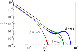
Figure 3: The cascade size distribution: numerical results (color lines), analytical results according to Eq. (10) (dashed lines) and the power-law decay with exponent $-3/2$ (thick solid line) for $N=10^{4}$, $\lambda=0.1$, $10^{7}$ time steps, and $\beta=0.001$ (red line, fastest decay), $\beta=0.01$ (green line, medium decay), $\beta=0.1$ (blue line, slowest decay). The analytical solution is not plotted for $\beta=0.1$ because it is very similar to that for $\beta=0.01$.

Finally, by comparing the empirical observations presented in Fig. 1 with the obtained analytical results, we can conclude that the presented model exhibits qualitative agreement with the studied real system.

3.4 Generalizations

To test how robust are the obtained results, we consider simple generalizations of the proposed model. First of all, when the multiplicative fragility update rule Eq. (2) is replaced by an additive one, the behavior of the system does not change considerably. The second generalization relates to the assumed even influence of a node’s failure on all the remaining nodes. Denoting the strength of failure propagation from node $i$ to node $j$ as $C_{i,j}$, the probability that node $j$ fails as a result of $i$’s failure can be generalized to $C_{i,j}f_{j}$. The probability that node $j$ fails as a result of a group $\mathcal{F}$ of failed nodes (given by Eq. (3) before) generalizes to the form

$$P_{F}(f_{j},\mathcal{F})=1-\prod_{i\in\mathcal{F}}(1-C_{i,j}f_{j}).$$ (14)

Matrix $\mathsf{C}$ encodes the structure of the network of node interactions.

When the elements $C_{i,j}$ are drawn independently from a given distribution and the system size is large, the mean-field approximation is again appropriate to describe the system behavior and the power-law size distribution with exponent $3/2$ results. Similarly when $\mathsf{C}$ contains a block structure with inter-block elements drawn from a different distribution than intra-block elements (this mimics the sector structure of the stock correlation matrix ManSta99 ; KimJe05 ), the original power-law size distribution remains largely unchanged (unless either the block division of $\mathsf{C}$ or one of the two probabilistic distributions are such that they do not allow to use the mean-field approximation). Analogous behavior results from the “random neighbor approximation” in which node’s neighbors are chosen anew repeatedly (see BDFJW94 for this kind of analysis of a different model).

When all elements $C_{i,j}$ are either zero or one, matrix $\mathsf{C}$ can be represented by a network and a complex topology of node interactions can be introduced by network models Newman03 . We studied two different types of networks: the Erdős-Rényi network where $C_{i,j}=1$ with probability $p$ and $C_{i,j}=0$ otherwise and the growing Barabási-Albert network where each new node is attached to $I$ old nodes. (These two kinds of networks are structurally very distinct as the former consists of nodes of approximately identical degree and the latter exhibits a power-law degree distribution.) Numerical results for both cases are shown in Fig. 4. As expected, for the Erdős-Rényi network with $p>1/N$, the size distribution exponent remains unchanged. When $p<1/N$, the network consists of small isolated components and hence big cascades cannot occur. The irregular size distribution $P(S)$ observed for $\beta=5\cdot 10^{-5}$ is due to topological properties of the particular network realization where the model was simulated (i.e., positions of respective ups and downs of the size distribution depend on the network realization). These results agree with a previous study of the sandpile dynamics Bona95 (see DoGoMe08 for an extensive recent review of critical phenomena in complex networks). By contrast, Barabási-Albert networks yield cascade size distributions with significantly higher exponents (approximately $1.65$) which is probably due to strong inhomogeneity of the network. When $I=1$, $P(S)$ deviates from a power law, probably as a consequence of the scale-free network topology (the same shape of the distribution is observed for different realizations of the network).

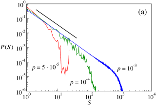
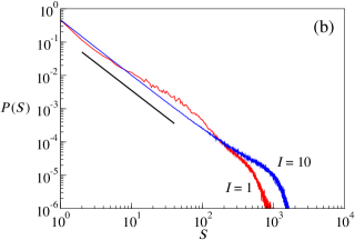
Figure 4: The cascade size distribution on complex networks: (a) sparse Erdős-Rényi networks with $p=5\cdot 10^{-5},10^{-4},10^{-3}$; the indicative thick line has slope $1.5$, (b) Barabási-Albert networks with $I=1$ and $I=10$; the indicative thick line has slope $1.65$). Parameters of the system: $N=10^{4}$, $\beta=0.005$, $\lambda=0.1$, $10^{7}$ time steps.

3.5 Role of the initial fragility values

While it sounds plausible that due to model’s stochasticity, the initial fragility values have no influence on the equilibrium fragility distribution, the situation is in fact more complicated. For example, a simple numerical simulation with $f_{i}(0)=1/N$ for all $i$ shows a case where: (i) no stationary fragility distribution arises, (ii) at any time step, only a small number of distinct fragility values is observed (see Fig. 5). What causes the discreteness of fragility values? Denoting the number of failing and healthy time steps of node $i$ as $F_{i}$ and $H_{i}$, respectively, it must hold that $F_{i}+H_{i}=t$ where $t$ is the current time step. This node’s fragility now can be written as

$$f_{i}(t)=f_{i}(0)(1+\beta)^{t}\big{[}\lambda/(1+\beta)\big{]}^{F_{i}}.$$ (15)

When all $f_{i}(0)$ are identical, the possible values of $f_{i}(t)$ are discrete at any time step $t$ and the ratio of neighboring possible values is $(1+\beta)/\lambda$. If $\lambda$ is small (as it is in our simulations), this ratio is large and hence the number of actually observed fragility values is small (because values much smaller or greater than the average fragility are unlikely). Eq. (15) implies that possible fragility values depend on $t$ and hence there can be no stationary fragility distribution—this is confirmed by Fig. 5 where fragility peaks constantly shift to higher values and change their relative heights. Interestingly, even this peculiar setting of $f_{i}(0)$ does not alter the long-term model’s behavior substantially and the aggregate quantities (such as the average failure probability or the cascade size distribution) are similar to those found for randomized initial fragility values before.

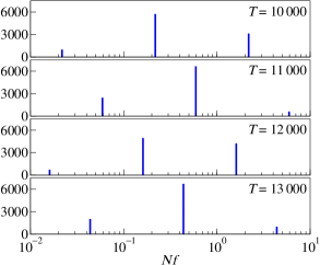
Figure 5: Fragility distributions at different time steps (the initial fragility values are set to $1/N$, $N=10^{4}$, $\beta=0.001$, $\lambda=0.1$).

Differences between neighboring peaks are $\lambda/(1+\beta)$, hence the time after which the fragility distribution pattern repeats can be estimated as $\ln\big{[}\lambda/(1+\beta)\big{]}/\ln(1+\beta)$. Since this is a typical time of fragility evolution, one can use it also as an estimate of the initial equilibration time $T_{\mathrm{eq}}$. For the smallest value of $\beta$ in our simulations ($\beta=0.005$) we obtain $T_{\mathrm{eq}}\approx 4\,600$ which ex post confirms our setting of the equilibration time to $10^{4}$. Finally, note that while the random setting of $f_{i}(0)$ prevents discrete fragility values from appearing, some remnants of the initial fragility values can be preserved by Eq. (15). To obtain a fragility distribution truly independent of the initial values, one has to assume annealed dynamics, i.e. fragility updating by randomized values of $\beta$ and $\lambda$.

4 Generalized model with partial memory

Fragility updating rules defined by Eq. (2) imply that nodes become more robust after a failure and hence autocorrelation of their failures as well as autocorrelation of the total number of failures are negative (their magnitudes depend on $\beta$ and $\lambda$). As discussed in Section 2, this is true for majority of stocks but certainly not for all of them. To allow for repeatedly failing stocks, we introduce the probability $\alpha$ with which a failed node stays failed also in the next time step (and consequently acts as an additional initial failed node). This probability has the role of partial memory in the system and, as we shall see, gives rise to volatility clustering and other effects observed in real financial data. Note that memory or delayed stress propagation are quite often part of cascade spreading models as in, for example, PeBuHe08 . We assume that fragilities of nodes which stay failed due to $\alpha$ are not updated in the given time step (when $\alpha$ is small, this assumption has little influence on the results).

Since $P(F)\ll 1$, the probability of a node’s repeated failure is now $P(F|F)\approx\alpha$ which, in combination with the empirical results presented in Section 2, motivates us to set $\alpha=0.04$. We further choose $\beta=0.01$ and $\lambda=0.1$ which best correspond to the critical regime in Fig. 3. Using this setting we numerically obtain conditional probabilities consistent with those observed in the empirical data: $P(F|F)=0.041$ (empirical value is $0.039$), $P(F)=0.004$ (empirical value is $0.003$) and $P(F|N)=0.004$ (empirical value is $0.003$). As long as we stay in the critical regime, these values depend on $\beta$ and $\lambda$ weakly. Presence of volatility clustering is confirmed by significantly positive autocorrelation of the number of failures $C(n_{F}(t),n_{F}(t+1))\approx 0.3$ (empirical value is $0.15$). The precise value depends on $\alpha$ and $\lambda$ (and much less on $\beta$) but positive autocorrelation naturally arises for $\alpha$ which is large enough. By contrast, $\alpha=0$ yields $P(F|F)\approx P(F)$ and $C(n_{F}(t),n_{F}(t+1))\approx-0.04$. Finally, Fig. 6 shows $P(S)$ for different values of $\alpha$. We see that for small values of $\alpha$, the size distribution remains power-law with exponent gradually decreasing as $\alpha$ grows. Due to the additional complexity introduced by partial memory, an analytical cascade size distribution for this generalized model has not been obtained yet.

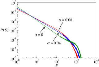
Figure 6: Cascade size distribution for the modified model: numerical results for $\beta=0.01$, $\lambda=0.1$, $N=10^{4}$, $10^{7}$ time steps, and various values of $\alpha$.

5 Discussion

We studied empirical stock prices and found that large simultaneous downturns follow a broad distribution consistent with a power law with exponent $2.19\pm 0.05$. To reproduce this behavior, we proposed a minimal stochastic model of failure propagation. Using a mean field approximation and branching process theory we derived the general cascade size distribution and determined the range of parameters which give rises to the critical regime. To reproduce other features observed in financial data, such as volatility clustering, partial memory was introduced within the basic model.

While our model implicitly assumes arrival of news to the market (they cause the initial nodes to fail and allow cascades to be created), we minimize the influence of news on the system’s behavior by assuming their equal impact (in each time step, exactly one initial node is chosen to fail). This approach is motivated by the extensive study of excess volatility which shows that it is difficult to link the observed trading volumes and volatility to the arriving information MiMu94 and even the large crash of 1987 does not seem to be triggered by particular news Black88 . In reality, of course, the impact of news on the market differs from one day to another. It could be therefore interesting to test how different ways of choosing the initial failed nodes influence the model’s behavior (for example, the number of the initial nodes can be random or network hubs may be preferentially chosen to trigger a cascade).

There is a number of other challenging questions which deserve further investigation. Firstly, since the cascade sizes corresponding to the secondary maximum in Fig. 3 are comparable with system size, this behavior cannot be described within the formalism of branching processes where an infinite system size is assumed. While we found an approximate condition for the appearance of the secondary maximum, how to proceed further towards an exhaustive description of the resulting size distribution is still an open question. Secondly, it would be interesting to find an analytical expression for the size distribution exponent in scale-free networks where it appears to differ from the mean-field value $3/2$. Thirdly, generalized model with “partial memory”, studied only numerically here, calls for analytical approaches. Fourthly, it would be interesting to know whether the model can be modified to produce power-law size distributions with exponents considerably higher than those reported here. One opportunity for such a generalization is to assume a dynamic network structure whose evolution depends on nodes’ failures, similarly to the approach used in BiMa04 ; CaGa09 for different models. Alternatively, as a generalization of the current binary model where nodes are either healthy or failed, one could define a multi or continuous-state model in which the probability of following a neighbor’s failure depends on the failure’s magnitude.

We stress that the probabilistic spreading mechanism proposed here is a general one and its use is not limited to market crashes or firm bankruptcies. For example, economic exchanges between countries are so intense that decline in one country may propagate to a neighboring one (take, for example, how growth in many European countries depends on spending of German consumers). On a two or three dimensional lattice, a similar mechanism might be employed to model earthquakes because, similarly to the proposed model, a failure at one place of the Earth’s crust exerts some stress on its neighborhood (the number of failed nodes would then represent the earthquake size). In summary, the proposed model, together with its generalizations, has proven to be simple yet rich in behavior. It poses a variety of new research questions and we are looking forward to its future development and applications.

- (1) M. Gladwell, The Tipping Point: How Little Things Can Make a Big Difference (Little Brown, New York, 2000).
- (2) I. Dobson, B. A. Carreras, V. E. Lynch, and D. E. Newman, Chaos 17, 026103 (2007).
- (3) J. Lorenz, S. Battiston, and F. Schweitzer, European Physical Journal B 71, 441 (2009).
- (4) D. Sornette, Physics Reports 378, 1 (2003).
- (5) B. H. Hong, K. E. Lee, and J. W. Lee, Physics Letters A 361, 6 (2007).
- (6) G. Weisbuch and S. Battiston, Journal of Economic Behavior and Organization 64, 448 (2007).
- (7) G. Iori and S. Jafarey, Physica A 299, 205 (2001).
- (8) P. Sieczka and J. A. Hołyst, European Physical Journal B 71, 461 (2009).
- (9) H. Iyetomi, H. Aoyama, Y. Fujiwara, and Y. Ikeda, W. Souma, arXiv:0901.1794 (2009).
- (10) D. Delli Gatti, M. Gallegati, B. C. Greenwald, A. Russo, and J. E. Stiglitz, Journal of Economic Interaction and Coordination 4, 195 (2009).
- (11) P. Bak, M. Paczuski, and M. Shubik, Physica A 246, 430 (1997).
- (12) R. Cont and J.-P. Bouchaud, Macroeconomic Dynamics 4, 170 (2000).
- (13) J. H. Miller and S. E. Page, Complex adaptive systems: An introduction to computational models of social life (Princeton University Press, Princeton, 2007).
- (14) P. Bak, C. Tang, and K. Wiesenfeld, Physical Review Letters 59, 381 (1987).
- (15) D. L. Turcotte, Reports on progress in physics 62, 1377 (1999).
- (16) C. Tang and P. Bak, Physical Review Letters 60, 2347 (1988).
- (17) H. Flyvbjerg, K. Sneppen, and P. Bak, Physical Review Letters 71, 4087 (1993).
- (18) P. Alstrøm, Physical Review A 38, 4905 (1988).
- (19) L. Pietronero, A. Vespignani, and S. Zapperi, Physical Review Letters 72, 1690 (1994).
- (20) M. Marsili, Europhysics Letters 28, 385 (1994).
- (21) D. Dhar, Physical Review Letters 64, 1613 (1990).
- (22) M. Paczuski, P. Bak, arXiv:cond-mat/9906077 (1999).
- (23) D. Sornette, Critical Phenomena in Natural Sciences, 2nd Ed. (Springer, Berlin, 2006).
- (24) A. Clauset, C. R. Shalizi, M. E. J. Newman, SIAM Review 51, 661 (2009).
- (25) V. Akgiray, The Journal of Business 62, 55 (1989).
- (26) R. N. Mantegna and H. E. Stanley, Introduction to Econophysics (Cambridge University Press, Cambridge, 1999).
- (27) R. Cont, in Long Memory in Economics, edited by G. Teyssière and A. P. Kirman (Springer, Heidelberg, 2007).
- (28) B. Mandelbrot, The Journal of Business 36, 394 (1963).
- (29) W. Feller, An Introduction to Probability Theory and Its Applications, Vol. 2 (Wiley, New York, 1970).
- (30) E. Ben-Naim and P. L. Krapivsky, Physical Review E 69, 050901(R) (2004).
- (31) T. E. Harris, The theory of branching processes (Dover, New York, 1989).
- (32) M. Dwass, Journal of Applied Probability 6, 682 (1969).
- (33) D. Sornette, Swiss Finance Institute Research Paper No. 09-36 (2009).
- (34) D.-H. Kim and H. Jeong, Physical Review E 72, 046133 (2005).
- (35) J. de Boer, B. Derrida, H. Flyvbjerg, A. D. Jackson, and T. Wettig, Physical Review Letters 73, 906 (1994).
- (36) M. E. J. Newman, SIAM Review 45, 167 (2003).
- (37) E. Bonabeau, Journal of the Physical Society of Japan 64, 327 (1995).
- (38) S. N. Dorogovtsev, A. V. Goltsev, and J. F. F. Mendes, Reviews of Modern Physics 80, 1275 (2008).
- (39) K. Peters, L. Buzna, and D. Helbing, International Journal of Critical Infrastructures 4, 46 (2008).
- (40) M. L. Mitchell and J. H. Mulherin, The Journal of Finance 49, 923 (1994).
- (41) F. Black, NBER Macroeconomics Annual 3, 269 (1988).
- (42) G. Bianconi and M. Marsili, Physical Review E 70, 035105(R) (2004).
- (43) G. Caldarelli and D. Garlaschelli, in Adaptive Networks: Theory, Models and Applications, edited by T. Gross and H. Sayama (Springer, Heidelberg, 2009).