Spin-orbit coupling and spectral function of interacting electrons in carbon nanotubes

Abstract

The electronic spin-orbit coupling in carbon nanotubes is strongly enhanced by the curvature of the tube surface and has important effects on the single-particle spectrum. Here, we include the full spin-orbit interaction in the formulation of the effective low-energy theory for interacting electrons in metallic single-wall carbon nanotubes and study its consequences. The resulting theory is a four-channel Luttinger liquid, where spin and charge modes are mixed. We show that the analytic structure of the spectral function is strongly affected by this mixing, which can provide an experimental signature of the spin-orbit interaction.

Spin-orbit interaction (SOI) effectswinkler are of great interest in the field of spintronics, and their detailed understanding is both of fundamental and of technological interest, e.g., for the coherent manipulation of spin qubits.spinqubit In single-wall carbon nanotubes (SWNTs) the SOI arises predominantly from the interplay of atomic SO coupling and curvature-induced hybridization, and its effect on the electronic bandstructure has recently been clarified.andoso ; prlale ; murphy ; chico ; rashbaale ; paco ; zhou ; jeong ; saito Contrary to other carbon-based materials, as, e.g., flat graphene, where SOI is very weak (of the order of few $\mu$eV), in SWNTs it can reach fractions of meV and has important consequences, previously overlooked. New experiments mceuen ; churchill on ultraclean SWNTs, made possible by advances in the fabrication technology, have indeed observed modifications of the electronic spectrum due to SOI. These results confirm the theoretical expectations, and motivate renewed interest on SOI in nanotubes. So far on the theory side the main focus has been on nanotube quantum dots,cntsodots where the SOI manifests itself in spectral features. Here we study long SWNTs, where long-ranged interactions can induce non-Fermi liquid electronic phases.ando In particular, without SOI, Luttinger liquid (LL) behaviorgogolin has been predicted for metallic SWNTs.egger97 Experimental evidence for this strongly correlated phase has been reported using quantum transportbockrath and photoemission spectroscopy.ishii

The question therefore arises how the LL theory of SWNTsegger97 is modified when the SOI is taken into account, and what are its observable consequences. This question is addressed and answered in detail below. Our main results are as follows. (i) The low-energy theory of metallic SWNTs still describes a Luttinger liquid. However, the decoupled plasmon modes do not correspond to spin and charge anymore. Spin-charge separation in the usual sensegogolin is therefore broken by the SOI. This effect can be traced back to a term in the SO Hamiltonian diagonal in sublattice space (see Eq. 1), which was previously overlooked. (ii) We discuss in detail the spectral function, a quantity that can directly be probed experimentally for SWNTs.ishii We show how the mixing of spin and charge modes due to SOI affects its analytic structure and modifies it from the established spinful LL behaviorgogolin ; meden . The predicted deviations are small but should be observable. (iii) The tunneling density of states, and hence most typical quantum transport observables, is only weakly affected by the SOI. This may explain why the SOI in SWNTs has long been overlooked. (iv) We shall clarify the similarities and the differences of the present SWNT theory to the LL description of 1D interacting semiconductor wires with Rashba SOI.moroz ; epl ; governale ; hausler ; gritsev ; oleg1 ; rkky

To start, let us address the bandstructure of a nominally metallic $(n,m)$ SWNT, where $2n+m\in 3\mathbb{Z}$. The chiral angleando is $\theta=\tan^{-1}[\sqrt{3}m/(2n+m)]$, and the tube radius is $R[{\rm nm}]\simeq 0.0391\sqrt{n^{2}+nm+m^{2}}$. We employ the effective SO Hamiltonian for $\pi$ electrons derived in Ref. saito, in the ${\bm{k}}\cdot{\bm{p}}$ scheme. This model is in semi-quantitative accordance with available experimental Coulomb blockade spectroscopy data,mceuen and summarizes earlier theoretical work. In particular, it includes the recently discovered “diagonal” contribution $E_{\rm SO}$, which is of crucial importance in our analysis (see below). Within this framework, the single-particle Hamiltonian $H_{0}({\bm{k}})$ for wavevector ${\bm{k}}=(k,k_{\perp})$ relative to the respective $K$ point is a $2\times 2$ matrix in sublattice space corresponding to the two basis atoms of the honeycomb lattice. This separately applies to both $K$ points $\alpha=\pm$ and both spin directions $\sigma=\pm$, where the spin quantization axis is along the tube axis. To leading order in the SOI, the spin label $\sigma$ is still a good quantum number.andoso ; prlale ; paco Periodic boundary conditions around the SWNT circumference imply a quantization of transverse momentum, $k_{\perp}R=n_{0}\in\mathbb{Z}$. We assume a Fermi energy $E_{F}>0$ but sufficiently small to justify that only the $n_{0}=0$ band has to be retained. All other bands are then separated by an energy gap $\approx\hbar v_{F}/R\approx 1$ eV, where $v_{F}\approx 8\times 10^{5}$ m/s. Then, $H_{0}(k)$ is given bysaito

$$\left(\begin{array}[]{cc}\alpha\sigma E_{\rm SO}&-\alpha\hbar v_{F}[\phi_{\perp}+i(k+\alpha\phi_{\parallel})]\\ -\alpha\hbar v_{F}[\phi_{\perp}-i(k+\alpha\phi_{\parallel})]&\alpha\sigma E_{\rm SO}\end{array}\right).$$ (1)

This form neglects trigonal warping corrections,ando which cause only tiny changes in the low-energy physics but would complicate our analysis substantially. Using the parameter estimates of Ref. saito, , the diagonal term is

$$E_{\rm SO}[\textrm{meV}]\simeq-\frac{0.135\cos(3\theta)}{R[\textrm{nm}]}.$$ (2)

Writing $\phi_{\perp}=\phi_{\perp,{\rm SO}}+\phi_{\perp,{\rm cur}}$, the SOI corresponds to a spin-dependent shift of the transverse momentum,paco ; mceuen ; saito

$$\phi_{\perp,{\rm SO}}[\textrm{nm}^{-1}]\simeq\alpha\sigma\frac{2.7\times 10^{-4}}{R[\textrm{nm}]},$$ (3)

while curvature effectssaito ; ando give

$$\phi_{\perp,{\rm cur}}[\textrm{nm}^{-1}] \simeq \frac{0.011\cos(3\theta)}{(R[\textrm{nm}])^{2}},$$

$$\phi_{\parallel}[\textrm{nm}^{-1}] \simeq \frac{0.045\sin(3\theta)}{(R[\textrm{nm}])^{2}}.$$

We remark that the Hamiltonian (1) contains the two leading effects of curvature-induced SOI, namely the diagonal contribution $E_{\rm SO}$ and the Rashba-type SOI encoded by $\phi_{\perp,{\rm SO}}$. Subleading terms, e.g., the “intrinsic” SOI,paco are much smaller and not taken into account here. The dispersion relation obtained from Eq. (1) is

$$E_{\pm}^{(\alpha,\sigma)}(k)=\alpha\sigma E_{\rm SO}\pm\hbar v_{F}\sqrt{\phi_{\perp}^{2}+(k+\alpha\phi_{\parallel})^{2}},$$ (4)

where the Kramers degeneracy is reflected in $E_{\pm}^{(\alpha,\sigma)}(k)=E^{(-\alpha,-\sigma)}_{\pm}(-k)$. Since $E_{F}>0$, only the conduction bands (positive sign) are kept, and the Fermi momenta $k^{(F)}_{r\alpha\sigma}$ for right- and left-movers ($r=R/L=\pm$) follow from $E^{(\alpha,\sigma)}_{+}\left(k^{(F)}_{r\alpha\sigma}\right)=E_{F}$, $k^{(F)}_{r\alpha\sigma}\approx r(E_{F}-\alpha\sigma E_{\rm SO})/\hbar v_{F}-\alpha\phi_{\parallel}$. We linearize the dispersion relation around the Fermi points, always assuming that $E_{F}$ is sufficiently far away from the band bottom. The 1D Fermi velocities $v_{\alpha,\sigma}=\hbar^{-1}\partial_{k}E^{(\alpha,\sigma)}_{+}\left(k=k^{(F)}_{+,\alpha\sigma}\right)$ take only two different values, $v_{A}\equiv v_{-,\uparrow}=v_{+,\downarrow}$ and $v_{B}\equiv v_{+,\uparrow}=v_{-,\downarrow}$. We mention in passing that $R/L$ movers have pairwise identical velocities only in the absence of trigonal warping and orbital magnetic fieldstsvelik or transverse fields,vishvesh as assumed here. It is convenient to introduce the mean velocity $v=(v_{A}+v_{B})/2$ and the dimensionless difference $\delta=(v_{A}-v_{B})/(2v)$. After some algebra, Eq. (4) together with the parameter estimates above yields

$$\frac{v}{v_{F}} \simeq 1-\frac{0.01(R[{\rm nm}])^{2}+17\cos^{2}(3\theta)}{(E_{F}[{\rm meV}])^{2}\ (R[{\rm nm}])^{4}},$$

$$\delta \simeq \frac{0.83\cos(3\theta)}{(E_{F}[{\rm meV}])^{2}\ (R[{\rm nm}])^{3}}.$$ (5)

The renormalization of $v$ away from $v_{F}$ goes always downwards, but the quantitative shift is small. The asymmetry parameter $\delta$ effectively parametrizes the SOI strength and is more important in what follows. For fixed $E_{F}$ and $R$, it is maximal for $\theta=0$ (zig-zag tube) and vanishes for $\theta=\pi/6$ (armchair tube). Moreover, $\delta$ increases for smaller tube radius, but the continuum description underlying our approach eventually breaks down for $R\lesssim 0.4$ nm. Since $E_{F}$ should at the same time be sufficiently far above the band bottom in Eq. (4), in practice this leads to rather small values, $\delta\lesssim 0.05$. This is a rather conservative estimate, though, based on the parameter values of Ref. saito, and larger values could be obtained if one uses different estimates. Nonetheless, we show below that observable consequences do arise.

The theory is then equivalently formulated using Abelian bosonization,gogolin which allows for the nonperturbative inclusion of interactions. We employ the boson fields $\phi_{\alpha}(x)$ with $\alpha=c+,c-,s+,s-$, representing the total and relative charge and spin density modes,egger97 and their conjugate momentum fields $\Pi_{\alpha}(x)=-\partial_{x}\theta_{\alpha}$, where $\theta_{\alpha}$ are the dual fields. Those fields are conveniently combined into the vectors $\Phi_{I}(x)=(\phi_{c+},\theta_{c+},\phi_{s-},\theta_{s-})^{T}$ and $\Phi_{0}(x)=(\phi_{c-},\theta_{c-},\phi_{s+},\theta_{s+})^{T}$. The important electron-electron forward scatteringfoot2 effects are parametrized by the standard LL parameter $K\equiv K_{c+}$, where $K=1$ for noninteracting electrons but $K\approx 0.2\ldots 0.4$ for SWNTs deposited on insulating substrates (or for suspended SWNTs) due to the long-ranged Coulomb interaction.egger97 ; bockrath ; ishii The low-energy Hamiltonian of a spin-orbit-coupled interacting metallic SWNT then reads

$$H=\frac{\hbar v}{2}\int dx\left(\begin{array}[]{c}\partial_{x}\Phi_{I}\\ \partial_{x}\Phi_{0}\end{array}\right)^{T}\left(\begin{array}[]{cc}{\bm{h}}(K)&0\\ 0&{\bm{h}}(1)\end{array}\right)\left(\begin{array}[]{c}\partial_{x}\Phi_{I}\\ \partial_{x}\Phi_{0}\end{array}\right)$$ (6)

with the $K$-dependent matrix

$${\bm{h}}(K)=\left(\begin{array}[]{cccc}\frac{1}{K^{2}}&0&\delta&0\\ 0&1&0&\delta\\ \delta&0&1&0\\ 0&\delta&0&1\end{array}\right).$$

The above representation shows that SOI ($\delta\neq 0$) breaks spin SU(2) symmetry. Notably, the modes $\Phi_{I}$ and $\Phi_{0}$ decouple, and interactions ($K\neq 1$) only affect the $\Phi_{I}$ sector. In each sector, the Hamiltonian is then formally identical to the one for a semiconductor wire with Rashba SOI in the absence of backscattering.rkky We consider a very long SWNT and ignore finite-length effects, i.e. the zero modes contributions to the Hamiltonian (6).

Equation (6) can be diagonalized by the linear transformationkimura $\Phi_{I}={\bm{V}}_{I}\Phi_{a}$ and $\Phi_{0}={\bm{V}}_{0}\Phi_{b}$, with the $4\times 4$ matrix

$${\bm{V}}_{I}=\left(\begin{array}[]{cccc}\cos\eta&0&-\frac{\sin\eta}{y}&0\\ 0&\cos\eta&0&-y\sin\eta\\ y\sin\eta&0&\cos\eta&0\\ 0&\frac{\sin\eta}{y}&0&\cos\eta\end{array}\right),$$ (7)

where

$$y=\sqrt{(1+K^{-2})/2},\quad\tan(2\eta)=\frac{2\delta y}{y^{2}-1}.$$ (8)

${\bm{V}}_{0}$ is as in Eq. (7) with $K=1$, i.e., $y=1$ and $\eta=\pi/4$. In terms of the new vectors $\Phi_{\rho}=(\phi_{+,\rho},\theta_{+,\rho},\phi_{-,\rho},\theta_{-,\rho})^{T}$ with mutually dual boson fields $\phi_{j\rho}$ and $\theta_{j\rho}$ for each set $(j=\pm,\rho=a/b)$, the diagonalized Hamiltonian is seen to describe a four-channel Luttinger liquid,

$$H=\sum_{j,\rho}\frac{\hbar v_{j\rho}}{2}\int dx\left(\frac{1}{K_{j\rho}}(\partial_{x}\phi_{j\rho})^{2}+K_{j\rho}(\partial_{x}\theta_{j\rho})^{2}\right).$$ (9)

The interacting sector corresponds to $\rho=a$, where the effective LL parameters $K_{\pm,a}$ and the plasmon velocities $v_{\pm,a}$ are

$$K_{\pm,a} = y^{\mp 1}\sqrt{\frac{3+K^{-2}\pm\Delta}{3K^{-2}+1\pm\Delta}},$$ (10)

$$\frac{v_{\pm,a}}{v} = \sqrt{y^{2}+\delta^{2}\pm\Delta/2},$$

$$\Delta = \sqrt{(K^{-2}-1)^{2}+(4\delta y)^{2}}$$

with $y$ in Eq. (8). For $\rho=b$, the noninteracting values apply, $K_{\pm,b}=1$ and $v_{\pm,b}=v(1\pm\delta)$. Note that the above expressions recover the LL theory for $\delta=0$,egger97 where $v_{j\rho}=v_{F}/K_{j\rho}$ with $K_{j\rho}=1$ except for $K_{+,a}=K$.

Within the framework of the LL Hamiltonian (9), using the bosonized form of the electron field operatorgogolin ; egger97 $\Psi_{r\alpha\sigma}(x,t)$ and the transformation (7), it is possible to obtain exact results for all observables of interest. In particular, arbitrary correlation functions of exponentials of the boson fields can be calculated. As an important application, we discuss here the spectral function for an $r=R/L$ moving electron with spin $\sigma$ near the $K$ point $\alpha=\pm$, which is defined as

$$A_{r\alpha\sigma}(q,\omega)=-\frac{1}{\pi}\ {\rm Im}\ G^{\rm ret}_{r\alpha\sigma}(q,\omega),$$ (11)

with the Fourier transform of the single-particle retarded Green’s function ($\Theta$ is the Heaviside function),

$$G^{\rm ret}_{r\alpha\sigma}(x,t)=-i\Theta(t)\left[\left\langle\Psi_{r\alpha\sigma}(x,t)\Psi^{\dagger}_{r\alpha\sigma}(0,0)\right\rangle+{\rm c.c.}\right],$$

and the momentum $q$ is measured with respect to the relative Fermi momentum $k^{(F)}_{r\alpha\sigma}$.

After some algebra, Eq. (11) follows in closed form, which we specify in the zero-temperature limit now. With the short-distance cutoff (lattice spacing) $a_{0}\approx 0.246$ nm, we find

$$A_{r\alpha\sigma}(q,\omega)\propto\int_{-\infty}^{\infty}dx\int_{-\infty}^{\infty}dt\ e^{-i[qx-\omega t]}$$ (12)

$$\times\Biggl{[}\prod_{j,\rho}\prod_{\mu=\pm}\left(1+i\frac{v_{j\rho}t+\mu rx}{a_{0}}\right)^{-\Gamma_{j,\rho;\mu}^{(\alpha\sigma)}}+(x,t)\to(-x,-t)\Biggr{]}$$

where the exponents for $j=\pm$ and $\mu=\pm$ are given by [see also Eq. (8)]

$$\Gamma_{j,a;\mu}^{(\alpha\sigma)} = \frac{1}{16}\Bigl{[}\cos(\eta)\left(K_{j,a}^{1/2}-\mu K_{j,a}^{-1/2}\right)$$

$$+ \alpha\sigma j\sin(\eta)\left(y^{j}K_{j,a}^{1/2}-\mu y^{-j}K^{-1/2}_{j,a}\right)\Bigr{]}^{2},$$

$$\Gamma_{j,b;\mu}^{(\alpha\sigma)} = \frac{1}{2}\delta_{j,\alpha\sigma}\delta_{\mu,-}.$$

The remaining Fourier integrals are difficult to perform. We here follow Ref. gogolin, and focus on the analytic structure of the spectral function, which can be obtained by the power counting technique and Jordan’s lemma. Up to an overall prefactor, the spectral function exhibits power-law singularities close to the lines $\omega=\pm v_{j\rho}q$. These singularities are captured by the approximate form

$$A_{r\alpha\sigma}(q,\omega) \approx \left(\prod_{j,\mu}\left|\omega+\mu rv_{j,a}q\right|^{\Gamma^{(\alpha\sigma)}-1-\Gamma_{j,a;\mu}^{(\alpha\sigma)}}\right)$$

$$\times \left|\omega-r(1+\alpha\sigma\delta)vq\right|^{\Gamma^{(\alpha\sigma)}-3/2}$$

$$\times \left[\Theta(\omega-r\bar{v}q)+\Theta(-\omega-rv_{-a}q)\right],$$

where $\bar{v}={\rm min}[v_{-,a},(1+\alpha\sigma\delta)v]$ and

$$\Gamma^{(\alpha\sigma)}=\sum_{j\rho\mu}\Gamma^{(\alpha\sigma)}_{j\rho\mu}.$$ (15)

We stress that Eq. (Spin-orbit coupling and spectral function of interacting electrons in carbon nanotubes) is asymptotically exact: it has the same analytic structure and the same exponents of the power laws at the singular lines $\omega=\pm v_{j\rho}q$ as the exact spectral function. Away from the singularities, however, it only serves illustrative purposes.

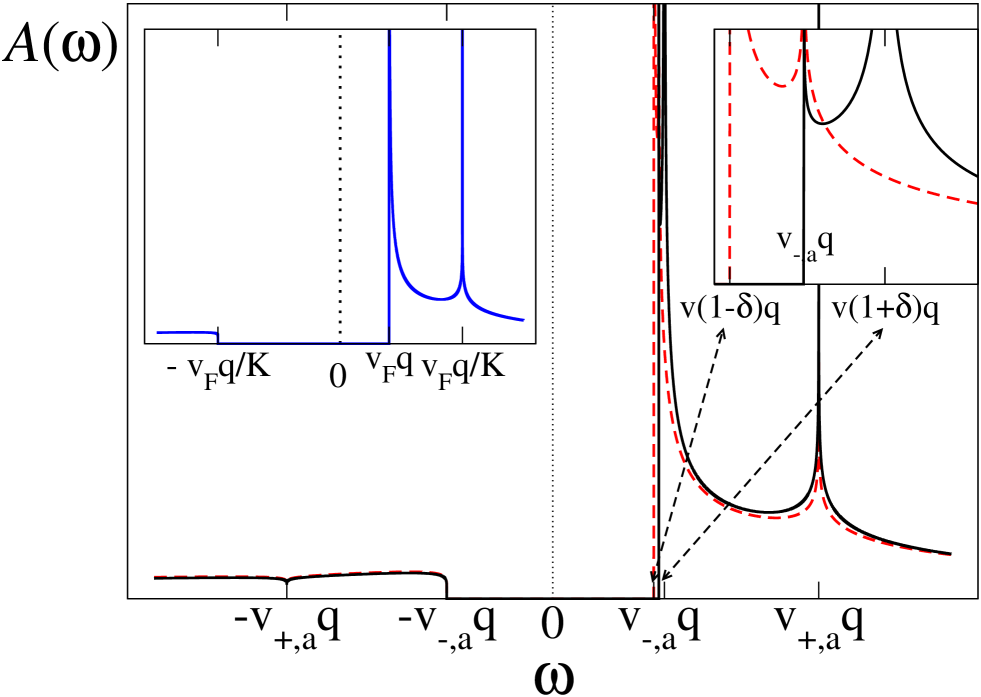
Figure 1: (Color online) Spectral function (Spin-orbit coupling and spectral function of interacting electrons in carbon nanotubes) for a right-mover in an interacting SWNT with LL parameter $K=0.4$ and SOI parameter $\delta=0.05$, shown in arbitrary units as function of $\omega$ for given wavevector $q>0$. The black solid curve is for $\alpha\sigma=+1$, while the red dashed curve is for $\alpha\sigma=-$. Note that $A_{R\alpha\sigma}(q,\omega)=0$ for $-v_{-,a}q<\omega<\bar{v}q$. Right inset: Magnified view around $\omega\approx v_{-,a}q$. Left inset: Same as main panel but without SOI ($\delta=0$). Shifts of the positions of the singularities due to the shifts of Fermi momenta are not included in the figure since each spectral function $A_{r\alpha\sigma}(q,\omega)$ is evaluated at momentum $q$ relative to the respective Fermi momentum.

The spectral function (Spin-orbit coupling and spectral function of interacting electrons in carbon nanotubes) is depicted in the main panel of Fig. 1 for fixed wavevector $q>0$ as a function of frequency $\omega$, taking $K=0.4$ and $\delta=0.05$. Compared to the well-known spectral function in the absence of SOI ($\delta=0$), see left inset of Fig. 1 and Refs. gogolin, ; meden, , additional structure can be observed for $\delta\neq 0$. First, the singular feature around $\omega=v_{-,a}q$ splits into two different power-law singularities when $\delta\neq 0$, see the right inset of Fig. 1 for a magnified view. For large $q$, the corresponding frequency differences are in the meV regime and can be resolved even for the rather small $\delta$ expected here. Second, for $-v_{+,a}q<\omega<-v_{-,a}q$, the spectral function is finite (albeit small) when $\delta\neq 0$. Note that for $\delta=0$, the respective velocities are $v_{+,a}=v_{F}/K$ and $v_{-,a}=v_{F}$, implying a large frequency window where this effect may take place. These predictions for the spectral function could be detected by photoemission spectroscopy.

Many standard quantum transport properties, however, will hardly show an effect due to the SOI, which may explain why effects of SOI in SWNTs have been so long overlooked. For instance, the tunneling density of states averaged over $(r,\alpha,\sigma)$ exhibits power-law scaling with $\omega$ for low frequencies, $\nu(\omega)\propto\omega^{\gamma-1}$. The exponent $\gamma$ is the smaller of the quantities $\Gamma^{(\pm)}$ in Eq. (15). This exponent is analytic in $\delta$, and the smallness of $\delta$ then implies that the tunneling density of states in SWNTs will be very close to the one in the absence of SOI. Let us also briefly comment on the relation of our results to the LL theory for semiconductor quantum wires with Rashba SOI.moroz ; epl ; governale ; hausler ; gritsev ; oleg1 ; rkky The “interacting” sector $\rho=a$ in Eq. (9) coincides with the semiconductor theory when electron-electron backscattering can be neglected. The additional presence of the “noninteracting” sector $\rho=b$, however, causes additional structure in the spectral function. Moreover, while backscattering in semiconductor wires is likely an irrelevant perturbation in the renormalization group sense,rkky it nonetheless causes a renormalization of the LL parameters and the plasmon velocities. Such renormalization effects are negligible in SWNTs.

To conclude, we have studied SOI effects on the effective low-energy theory of interacting metallic SWNTs. We have shown that a four-channel Luttinger liquid theory remains applicable, but compared to the previous formulation without SOI,egger97 all four channels are now characterized by different Luttinger liquid parameters and plasmon velocities, reflecting the broken spin $SU(2)$ symmetry. The coupling of spin and charge modes leads then to observable modifications in the spectral function, which provide an experimental signature of SOI. This work was supported by the SFB TR 12 of the DFG.

References

- (1) R. Winkler, Spin-Orbit Coupling Effects in Two-Dimensional Electron and Hole Systems (Springer, Berlin, 2003).
- (2) C. Flindt, A.S. Sørensen, and K. Flensberg, Phys. Rev. Lett. 97, 240501 (2006); D.V. Bulaev, B. Trauzettel, and D. Loss, Phys. Rev. B 77, 235301 (2008).
- (3) T. Ando, J. Phys. Soc. Jpn. 69, 1757 (2000).
- (4) A. De Martino, R. Egger, K. Hallberg, and C.A. Balseiro, Phys. Rev. Lett. 88, 206402 (2002).
- (5) A. De Martino, R. Egger, F. Murphy-Armando, K. Hallberg, J. Phys. Cond. Matt. 16, S1437 (2004).
- (6) L. Chico, M.P. Lopez-Sancho, and M.C. Munoz, Phys. Rev. Lett. 93, 176402 (2004); Phys. Rev. B 79, 235423 (2009).
- (7) A. De Martino and R. Egger, J. Phys. Cond. Matt. 17, 5523 (2005).
- (8) D. Huertas-Hernando, F. Guinea, and A. Brataas, Phys. Rev. B 74, 155426 (2006).
- (9) J. Zhou, Q. Liang, and J. Dong, Phys. Rev. B 79, 195427 (2009).
- (10) J.S. Jeong and H.W. Lee, Phys. Rev. B 80, 075409 (2009).
- (11) W. Izumida, K. Sato, and R. Saito, J. Phys. Soc. Jpn. 78, 074707 (2009).
- (12) F. Kuemmeth, S. Ilani, D.C. Ralph, and P.L. McEuen, Nature 452, 448 (2008).
- (13) H.O.H. Churchill, F. Kuemmeth, J.W. Harlow, A. J. Bestwick, E. I. Rashba,1, K. Flensberg, C. H. Stwertka, T. Taychatanapat, S. K. Watson, and C. M. Marcus, Phys. Rev. Lett. 102, 166802 (2009).
- (14) B. Wunsch, Phys. Rev. B 79, 235408 (2009); A. Secchi and M. Rontani, Phys. Rev. B 80, 041404(R) (2009); M.R. Galpin, F.W. Jayatilaka, D.E. Logan, and F.B. Anders, Phys. Rev. B 81, 075437 (2010).
- (15) For reviews, see: T. Ando, J. Phys. Soc. Jpn. 74, 777 (2005); J.C. Charlier, X. Blase, and S. Roche, Rev. Mod. Phys. 79, 677 (2007).
- (16) For a textbook discussion, see A.O. Gogolin, A.A. Nersesyan, and A.M. Tsvelik, Bosonization and Strongly Correlated Systems (Cambridge University Press, Cambridge, 1998).
- (17) R. Egger and A.O. Gogolin, Phys. Rev. Lett. 79, 5082 (1997); Eur. Phys. J. B 3, 281 (1998); C. Kane, L. Balents, and M.P.A. Fisher, Phys. Rev. Lett. 79, 5086 (1997).
- (18) M. Bockrath et al., Nature 397, 598 (1999); Z. Yao, H.W.C. Postma, L. Balents, and C. Dekker, Nature 402, 273 (1999); B. Gao, A. Komnik, R. Egger, D.C. Glattli, and A. Bachtold, Phys. Rev. Lett. 92, 216804 (2004).
- (19) H. Ishii et al., Nature 426, 540 (2003).
- (20) O.M. Auslaender et al., Science 308, 88 (2005); Y. Jompol et al., Science 325, 597 (2009).
- (21) V. Meden and K. Schönhammer, Phys. Rev. B 46, 15753 (1992); Phys. Rev. B 47, 16205 (1993); J. Voit, Phys. Rev. B 47 6740 (1993).
- (22) A.V. Moroz, K.V. Samokhin, and C.H.W. Barnes, Phys. Rev. Lett. 84, 4164 (2000); Phys. Rev. B 62, 16900 (2000).
- (23) A. De Martino and R. Egger, Europhys. Lett. 56, 570 (2001).
- (24) M. Governale and U. Zülicke, Phys. Rev. B 66, 073311 (2002).
- (25) W. Häusler, Phys. Rev. B 70, 115313 (2004).
- (26) V. Gritsev, G.I. Japaridze, M. Pletyukhov, and D. Baeriswyl, Phys. Rev. Lett. 94, 137207 (2005).
- (27) J. Sun, S. Gangadharaiah, and O.A. Starykh, Phys. Rev. Lett. 98, 126408 (2007).
- (28) A. Schulz, A. De Martino, P. Ingenhoven, and R. Egger, Phys. Rev. B 79, 205432 (2009).
- (29) A. De Martino, R. Egger, and A.M. Tsvelik, Phys. Rev. Lett. 97, 076402 (2006).
- (30) W. DeGottardi, T.-C. Wei, and S. Vishveshwara, Phys. Rev. B 79, 205421 (2009).
- (31) Electron-electron backscattering effects in SWNTs are tinyegger97 and disregarded here. Moreover, we stay away from half-filling such that Umklapp scattering processes also play no role.
- (32) T. Kimura, K. Kuroki, and H. Aoki, Phys. Rev. B 53, 9572 (1996).