The Hamburg/ESO R-process Enhanced Star survey (HERES)

Abstract

Aims. We report on a detailed abundance analysis of the strongly r-process enhanced giant star newly discovered in the HERES project, HE 2327$-$5642 ([Fe/H] = –2.78, [r/Fe] = +0.99).

Methods. Determination of stellar parameters and element abundances was based on analysis of high-quality VLT/UVES spectra. The surface gravity was calculated from the non-local thermodynamic equilibrium (NLTE) ionization balance between Fe i and Fe ii, and Ca i and Ca ii.

Results. Accurate abundances for a total of 40 elements and for 23 neutron-capture elements beyond Sr and up to Th were determined in HE 2327$-$5642. For every chemical species, the dispersion of the single line measurements around the mean does not exceed 0.11 dex. The heavy element abundance pattern of HE 2327$-$5642 is in excellent agreement with those previously derived for other strongly r-process enhanced stars such as CS 22892-052, CS 31082-001, and HE 1219-0312. Elements in the range from Ba to Hf match the scaled Solar $r$-process pattern very well. No firm conclusion can be drawn with respect to a relationship between the fisrt neutron-capture peak elements, Sr to Pd, in HE 2327$-$5642 and the Solar $r$-process, due to the uncertainty of the latter. A clear distinction in Sr/Eu abundance ratios was found between the halo stars with different europium enhancement. The strongly r-process enhanced stars reveal a low Sr/Eu abundance ratio at [Sr/Eu] = $-0.92\pm 0.13$, while the stars with $0<$ [Eu/Fe] $<1$ and [Eu/Fe] $<0$ have 0.36 dex and 0.93 dex larger Sr/Eu values, respectively. Radioactive dating for HE 2327$-$5642 with the observed thorium and rare-earth element abundance pairs results in an average age of 13.3 Gyr, when based on the high-entropy wind calculations, and 5.9 Gyr, when using the Solar r-residuals. HE 2327$-$5642 is suspected to be radial-velocity variable based on our high-resolution spectra, covering $\sim 4.3$ years.

1 Introduction

The detailed chemical abundances of Galactic halo stars contain unique information on the history and nature of nucleosynthesis in our Galaxy. A number of observational and theoretical studies have established that in the early Galaxy the rapid ($r$) process of neutron captures was primarily responsible for formation of heavy elements beyond the iron group (we cite only the pioneering papers of Spite & Spite, 1978; Truran, 1981). The onset of the slow ($s$) process of neutron captures occurred at later Galactic times (and higher metallicities) with the injection of nucleosynthetic material from long-lived low- and intermediate-mass stars into the interstellar medium (see Travaglio et al., 1999, and references therein). Since 1994, a few rare stars have been found that exhibit large enhancements of the $r$-process elements, as compared to Solar ratios, suggesting that their observed abundances are dominated by the influence of a single, or at most very few nucleosynthesis events. The $r$-process is associated with explosive conditions of massive-star core-collapse supernovae (Woosley et al., 1994), although the astrophysical site(s) of the $r$-process has yet to be identified. Observations of the stars with strongly enhanced $r$-process elements have placed important constraints on the astrophysical site(s) of their synthesis.

Sneden et al., (1994) found that the extremely metal-poor ([Fe/H] $\sim-3.1$) giant CS 22892-052 is neutron-capture-rich, [Eu/Fe]$\simeq+1.6$ (following the suggestion of Beers & Christlieb, 2005, we hereafter refer to stars having $\mathrm{[Eu/Fe]}>+1$ and $\mathrm{[Ba/Eu]}<0$ as r-II stars), and that the relative abundances of nine elements in the range from Ba to Dy are consistent with a scaled Solar system $r$-process abundance distribution. Later studies of CS 31082-001 (Hill et al., 2002), BD+17^∘ 3248 (Cowan et al., 2002), CS 22892-052 (Sneden et al., 2003), HD 221170 (Ivans et al., 2006), CS 22953-003 (François et al., 2007), HE 1219-0312 and CS 29491-069 (Hayek et al., 2009) provided strong evidence for a universal production ratio of the second $r$-process peak elements from Ba to Hf during the Galaxy history. CS 31082-001 (Hill et al., 2002) provided the first solid evidence that variations in progenitor mass, explosion energy, and/or other intrinsic and environmental factors may produce significantly different $r$-process yields in the actinide region ($Z\geq 90$). The third $r$-process peak ($76\leq Z\leq 83$) is so far not well constrained, because, in most r-II stars, it is only sampled by abundance measurements of two elements, Os and Ir. The abundances of platinum and gold were obtained for CS 22892-052 (Sneden et al., 2003). The only detection of lead in a r-II star so far is in CS31082-001 (Plez et al., 2004).

Sneden et al., (2003) reported an underabundance of elements in the range of $40<Z<56$ relative to the scaled Solar $r$-process, which prompted a discussion of multiple $r$-process sites (see, for example, Travaglio et al., 2004; Qian & Wasserburg, 2008; Farouqi et al., 2009). The detection of the radioactive elements thorium and uranium provided new opportunities to derive the ages of the oldest stars and hence to determine a lower limit for the age of the Universe (see the pioneering papers of Sneden et al., 1996; Cayrel et al., 2001). It appears that all the r-II stars with measured Th (and U) can be devided into two groups: (a) stars exhibiting an actinide boost (e.g., CS 31082-001, HE 1219-0312), and (b) stars with no obvious enhancement of thorium with respect to the scaled Solar r-process pattern (e.g., CS 22892-052, CS 29497-004; for a full list of stars, see Roederer et al., 2009). For the actinide boost stars, ages cannot be derived when only a single radioactive element, either Th or U, is detected.

To make clear an origin of the heavy elements beyond the iron group in the oldest stars of the Galaxy, more and better measurements of additional elements are required. Currently, there are about ten r-II stars reported in the literature (Hill et al., 2002; Sneden et al., 2003; Christlieb et al., 2004; Honda et al., 2004; Barklem et al., 2005; François et al., 2007; Frebel et al., 2007; Lai et al., 2008; Hayek et al., 2009). Abundance pattern for a broad range of nuclei, based on high-resolution spectroscopic studies, have been reported for only six of these stars.

Continuing our series of papers on the Hamburg/ESO R-process-Enhanced Star survey (HERES), we aim at extending our knowledge about synthesis of heavy elements in the early Galaxy by means of a detailed abundance analysis of the strongly $r$-process enhanced star HE 2327$-$5642. In our study we also investigate the reliability of multiple Th/$X$ chronometers for HE 2327$-$5642, where $X$ is an element in the Ba–Hf range.

HE 2327$-$5642 was identified as a candidate metal-poor star in the Hamburg/ESO Survey (HES; see Christlieb et al., (2008) for details of the candidate selection procedures). Moderate-resolution ($\Delta\lambda=2$ Å) spectroscopy obtained at the Siding Spring Observatory (SSO) 2.3 m-telescope with the Double Beam Spectrograph (DBS) confirmed its metal-poor nature. Therefore, it was included in the target list of the HERES project. A detailed description of the project and its aims can be found in Christlieb et al., (2004, hereafter Paper I), and methods of automated abundance analysis of high-resolution “snapshot” spectra have been described in Barklem et al., (2005, hereafter Paper II). “Snapshot” spectra having $R\sim 20,000$ and $S/N\sim 50$ per pixel at 4100 Å revealed that HE 2327$-$5642 exhibits strong overabundances of the $r$-process elements, with [Eu/Fe] = $+1.22$ and $\mathrm{[Ba/Eu]}=-0.56$ (Paper II).

This paper is structured as follows. After describing the observations (Section 2), we report on the abundance analysis of HE 2327$-$5642 in Sections 3 and 4, based on high-quality VLT/UVES spectra and MAFAGS model atmospheres (Fuhrmann et al., 1997). The heavy element abundance pattern of HE 2327$-$5642 is discussed in Section 5. Section 6 reports on the radioactive decay age determination. Conclusions are given in Section 7.

2 Observations

For the convenience of the reader, we list the coordinates and photometry of HE 2327$-$5642 in Table 1. The photometry was taken from Beers et al., (2007). High-quality spectra of this star was acquired during May–November 2005 with the VLT and UVES in dichroic mode. The BLUE390$+$RED580 (4 h total integration time) and BLUE437$+$RED860 (10 h) standard settings were employed to ensure a large wavelength coverage. The slit width of $0.8^{\prime\prime}$ in both arms yielded a resolving power of $R=60,000$. A $1\times 1$ pixel binning ensured a proper sampling of the spectra. The observations are summarized in Table 2.

The pipeline-reduced spectra were shifted to the stellar rest frame and then co-added in an iterative procedure in which pixels in the individual spectra affected by cosmic ray hits not fully removed during the data reduction, affected by CCD defects, or other artifacts, were identified. These pixels were flagged and ignored in the final iteration of the co-addition. Both co-added blue spectra have a signal-to-noise ratio ($S/N$) of at least 50 per pixel at $\lambda>3800$ Å. At the shortest wavelengths, the $S/N$ of the BLUE390 and BLUE437 is $10$ (at 3330 Å) and 70 (at 3756 Å), respectively. The red arm spectra have $S/N>100$ per pixel in most of the covered spectral range.

Table 1: Coordinates and photometry of HE 2327$-$5642.

R.A.(2000.0)	23:30:37.2
dec.(2000.0)	$-$56:26:14
$V$	$13.881\pm 0.003$
$B-V$	$0.709\pm 0.005$
$V-R$	$0.456\pm 0.004$
$V-I$	$0.933\pm 0.005$

Table 2: VLT/UVES observations of HE 2327$-$5642.

Setting	$\lambda^{1}$	$t_{\mbox{\scriptsize exp}}$	$S/N^{2}$
BLUE390	$3330$–$4510$ Å	$4.0$ h	$10$–$65$
BLUE437	$3756$–$4978$ Å	$10.0$ h	$70$–$120$
REDL580	$4785$–$5745$ Å	$4.0$ h	$100$–$120$
REDU580	$5830$–$6795$ Å	$4.0$ h	$60$–$120$
REDL860	$6700$–$8508$ Å	$10.0$ h	$100$–$180$
1  $\lambda$ refers to rest frame wavelengths,
2  $S/N$ refers to the signal-to-noise ratio per pixel.

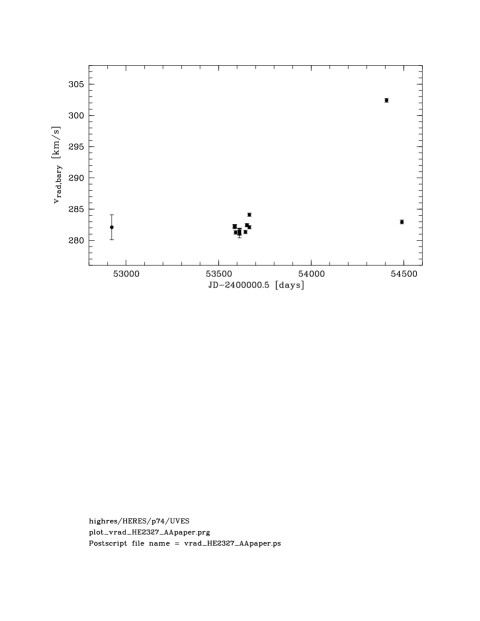
Figure 1: Radial velocity measurements of HE 2327$-$5642.

Barycentric radial velocities of HE 2327$-$5642 as measured with Gaussian fits of selected absorption lines in our high-resolution spectra, covering $\sim 4.3$ years, indicate that the star is radial-velocity variable, although no signatures of a double-lined spectroscopic binary star were found. The data taken during the Modified Julian Date (MJD) period $53587.2$–$53666.2$ (Table 3) suggests that the radial velocity varies on timescales of $\sim 10$ days, and that the radial velocity curve went through a minimum approximately at MJD 53620 (see Fig. 1). Furthermore, the measurement at MJD $54407.019$ deviates by $\sim 20$ km/s from the average of the radial velocities measured at the other epochs, and by a similar amount from the measurement taken only about three months later. The available data cannot be fitted satisfactorily by a sinusoidal curve, and therefore we suspect that the orbit of the system is highly elliptical. Additional observations are needed to confirm the variability, and for determining the period as well as the nature of the orbit.

Table 3: Barycentric radial velocities $v_{\mbox{\scriptsize rad,bary}}$ of HE 2327$-$5642.

MJD∗	$v_{\mbox{\scriptsize rad,bary}}$	$\sigma^{**}$
$\mathrm{[days]}$	[km/s]	[km/s]
$52923.137$	$282$	$2$
$53587.172$	$282.2$	$0.3$
$53587.215$	$282.3$	$0.2$
$53587.257$	$282.3$	$0.3$
$53587.321$	$282.2$	$0.3$
$53592.289$	$281.3$	$0.3$
$53613.092$	$281.3$	$0.4$
$53613.135$	$281.5$	$0.5$
$53613.178$	$281.1$	$0.7$
$53613.221$	$281.4$	$0.6$
$53645.081$	$281.3$	$0.3$
$53653.044$	$282.4$	$0.2$
$53653.087$	$282.4$	$0.2$
$53666.112$	$284.1$	$0.2$
$53666.157$	$284.0$	$0.2$
$54407.020$	$302.4$	$0.3$
$54490.027$	$282.9$	$0.3$
∗ The date refers to the start of the exposure.
∗∗ The error bars are the 1 $\sigma$ scatter of the
measurements based on different lines.

3 Analysis method

Our determinations of the stellar parameters and the elemental abundances are based on line profile and equivalent width analyses. We ignored any lines with equivalent widths larger than 100 mÅ. An exception is the elements, such as strontium, where only strong lines can be detected in HE 2327$-$5642. For a number of chemical species, namely, H i, Na i, Mg i, Al i, Ca i-ii, and Fe i-ii, non-local thermodynamic equilibrium (NLTE) line formation was considered. The theoretical spectra of the remaining elements were calculated assuming LTE. The coupled radiative transfer and statistical equilibrium equations were solved with the code NONLTE3 (Sakhibullin, 1983; Kamp et al., 2003) for H i  and Na i, and an updated version of the DETAIL code (Butler & Giddings, 1985) for the remaining NLTE species. The departure coefficients were then used to calculate the synthetic line profiles with the code SIU (Reetz, 1991). The metal line list has been extracted from the VALD database (Kupka et al., 1999). For molecular lines, we applied the data compiled by Kurucz, (1994). In order to compare with observations, computed synthetic profiles are convolved with a profile that combines instrumental broadening with a Gaussian profile of 3.6 km s^-1 and broadening by macroturbulence. We employ the macroturbulence parameter $V_{\rm mac}$ in the radial-tangential form as prescribed in Gray, (1992). From analysis of many line profiles in the spectrum of HE 2327$-$5642, $V_{\rm mac}$ = 3.3 km s^-1 was empirically found with some allowance to vary by $\pm$0.3 km s^-1 (1$\sigma$).

The abundance analysis based on equivalent widths was performed with the code WIDTH9 (Kurucz, 2004). The SIU and WIDTH9 codes both treat continuum scattering correctly; i.e., scattering is taken into account not only in the absorption coefficient, but also in the source function.

Both in SIU and WIDTH9, we used the updated partition functions from the latest release of the MOOG code (Sneden, 1973), with exception of Ho ii and Ir ii. For Ho ii, we adopted the partition function calculated by Bord & Cowley, (2002). The Ir ii partition function was revised based on the measured energy levels from van Kleef & Metsch, (1978). For the temperature range we are concerned with this makes a difference of +0.08/ +0.2 dex in the Ho/Ir abundance determined from the Ho ii/Ir i lines.

3.1 Stellar parameters and atmospheric models

In Paper II, an effective temperature of $5048\pm 100$ K was derived from photometry when adopting the reddening derived from the maps of Schlegel et al., (1998). A subsequent analysis of the snapshot spectrum gave $\log g=2.22\pm 0.25$ and [Fe/H] = $-2.95\pm 0.12$. For the stellar parameter determination and abundance analysis, we use plane-parallel, LTE, and line-blanketed MAFAGS model atmospheres (Fuhrmann et al., 1997). Enhancements of the $\alpha$-elements Mg, Si, and Ca by the amounts determined in a close-to-final iteration of our analysis were taken into account when computing these model atmospheres. Since suitable lines of oxygen are not covered by our spectra, we could not determine the oxygen abundance, hence we adopted $\mathrm{[O/Fe]}=+0.5$, which is a typical value of other stars at the metallicity of HE 2327$-$5642. It is worth noting that oxygen in cool stellar atmospheres plays a minor role as a donator of free electrons and as an opacity source, hence an uncertainty in the oxygen abundance does not significantly affect the calculated atmospheric structure.

Heiter & Eriksson, (2006) investigated the effect of geometry on atmospheric structure and line formation for Solar abundance models, and concluded that plane-parallel models can be applied in abundance analysis for the stars with $\log g>2$ and $T_{\mbox{\scriptsize eff}}>4000$ K. Therefore, HE 2327$-$5642 lies in the stellar parameter range where the usage of plane-parallel models is appropriate. This is confirmed by flux and abundance comparisons between a MAFAGS plane-parallel and MARCS (Gustafsson et al., 2008) spherical models with stellar parameters close to those of HE 2327$-$5642; i.e., $T_{\mbox{\scriptsize eff}}/\log g/\mathrm{[M/H]}=5000/2.0/-3$. Synthetic spectra were computed in the wavelength range 3500–16,000 Å with the code SIU, which solves the equation of radiative transfer in only one depth variable. For the absolute flux, we compared three different combinations of model atmosphere and spectrum synthesis geometries: consistently plane-parallel (MAFAGS + SIU, $p-p$), inconsistent (MARCS + SIU, $s-p$), and consistently spherical (MARCS model atmosphere library, $s-s$). The difference in absolute flux between these three models does not exceed 0.001 dex for wavelengths longer than 6600 Å. For $\lambda<6600$ Å, the $p-p$ and $s-p$ fluxes are lower than that from the $s-s$ model with a maximum difference of 0.01 dex and 0.02 dex, respectively, at wavelengths around 3500 Å.

In Fig. 2, we show the line profiles of H$\alpha$ and H$\gamma$ for all three models. The H$\gamma$ profile from the MAFAGS model is consistent with that from the $s-s$ model. The difference in H$\alpha$ relative fluxes between the MAFAGS and $s-s$ models translates to an effective temperature difference of 60 K. The abundance differences for the selected spectral lines were obtained between the $p-p$ and $s-p$ models by fitting the calculated synthetic spectra to the observed ones. The difference in absolute abundances, $\Delta\log\varepsilon((p-p)-(s-p))$, is always negative, but does not exceed 0.01 and 0.02 dex for the lines of neutral and ionized species, respectively. The differences in abundance ratios are also negligible; i.e., smaller than 0.01 dex.

Figure 2: Synthetic profiles of H$\alpha$ (top panel) and H$\gamma$ (bottom panel) from the $s-s$ (dashed curve), $s-p$ (continuous curve), and $p-p$ (dotted curve) models. The calculations for the $s-p$ and $p-p$ models were made for pure hydrogen lines.

Figure 3: Top panel: synthetic flux profile of H$\gamma$ computed for $T_{\mbox{\scriptsize eff}}=5000$ K (continuous curve) compared to the observed spectrum of HE 2327$-$5642 (bold dots). The dashed curves show the effect of a 80 K variation in the effective temperature on the synthetic spectrum. In all calculations, we assumed $\log g=2.3$, $\mathrm{[Fe/H]}=-2.95$, and $\xi=1.7$ km s^-1. Bottom panel: effective temperature derived from the H$\alpha$ (filled circles) and H$\gamma$ (open diamonds) line wings in HE 2327$-$5642 as a function of surface gravity. The error bars show the uncertainty of $T_{\mbox{\scriptsize eff}}$ arising from profile fitting.

The effective temperature of HE 2327$-$5642 was also determined from a profile analysis of H$\alpha$ and H$\gamma$ based on NLTE line formation calculations of H i using the method described by Mashonkina et al., (2008). Only these two lines were employed because an accurate continuum rectification was not possible in the spectral regions covering other Balmer lines. The metallicity and microturbulence velocity from Paper II were adopted during the analysis of these Balmer lines, while the gravity was varied between $\log g=1.8$ and 2.4. The theoretical profiles of H$\alpha$ and H$\gamma$ were computed by convolving the profiles resulting from the thermal, natural, and Stark broadening (Vidal et al., 1970, 1973), as well as self-broadening. For the latter, we use the self-broadening formalism of Barklem et al., (2000).

We obtained weak NLTE effects for the H$\gamma$ profile beyond the core, such that the difference in $T_{\mbox{\scriptsize eff}}$ derived from this line between NLTE and LTE does not exceed 20 K. It was also found that the H$\gamma$ line wings are insensitive to a variation in surface gravity in the stellar parameter range we are concerned with. The best fit is achieved at $T_{\mbox{\scriptsize eff}}=5000$ K. Figure 3 (top panel) illustrates the quality of the fits.

Based on the $S/N$ ratio of the observed spectrum and the sensitivity of the Balmer lines to variations of $T_{\mbox{\scriptsize eff}}$, we estimate the uncertainty of $T_{\mbox{\scriptsize eff}}$ arising from profile fitting as 50 K for each line. For H$\alpha$, NLTE leads to a weakening of the core-to-wing transition compared to the LTE case, resulting in a 80–100 K higher $T_{\mbox{\scriptsize eff}}$, depending on surface gravity. The effective temperature of HE 2327$-$5642 obtained from H$\alpha$ is also dependent on $\log g$, as shown in bottom panel of Fig. 3. The temperature deduced from combining the analyses of H$\alpha$ and H$\gamma$ is $T_{\mbox{\scriptsize eff}}=5000\pm 70$ K, and a favorable range of $\log g$ is between 1.95 and 2.40.

The surface gravity and microturbulence velocity were redetermined from Ca and Fe lines based on NLTE line formation for Ca i-ii and Fe i-ii, using the methods of Mashonkina et al., (2007); Mashonkina et al., 2009a . For Ca i-ii, we employ the lines listed in Mashonkina et al., (2007) along with the atomic data on $gf-$values and van der Waals damping constant. In total, 8 lines of Ca i and the only suitable Ca ii line covered by our spectra, at 8498 Å, were used. For Fe i-ii, 49 lines of Fe i and 8 lines of Fe ii were selected from the linelists of Mashonkina et al., 2009a , Paper II, Jonsell et al., (2006), and Ivans et al., (2006). Van der Waals broadening of the Fe lines was accounted for with the most accurate data available from calculations of Anstee & O’Mara, (1995); Barklem & O’Mara, (1997, 1998); Barklem et al., (1998); Barklem & Aspelund-Johansson, (2005). Hereafter, these collected papers by Anstee, Barklem, and O’Mara are referred to as the $ABO$ theory. The lines used are listed in Table LABEL:linelist (Online material) together with transition information, references for the adopted $gf-$values, and final element abundances.

For Ca and Fe, we apply a line-by-line differential NLTE approach, in the sense that stellar line abundances are compared with individual abundances of their Solar counterparts. It is worth noting that, with the adopted atomic parameters, the absolute Solar NLTE abundances obtained from the two ionization stages, Ca i and Ca ii, Fe i and Fe ii, were consistent within the error bars: $\log\varepsilon_{\rm\odot}$(Ca i) = $6.36\pm 0.06$, $\log\varepsilon_{\rm\odot}$(Ca ii 8498 Å) = $6.29$, $\log\varepsilon_{\rm\odot}$(Fe i) = $7.47\pm 0.10$, and $\log\varepsilon_{\rm\odot}$(Fe ii) = $7.46\pm 0.07$ (we refer to abundances on the usual scale, where $\log\varepsilon_{\rm H}=12$).

NLTE computations were performed for a small grid of model atmospheres with two effective temperatures, namely $T_{\mbox{\scriptsize eff}}=5050$ K, as derived from photometry, and $T_{\mbox{\scriptsize eff}}=4980$ K, which is close to the result of the Balmer line analysis. In the statistical equilibrium calculations, inelastic collisions with hydrogen atoms were accounted for, using the Steenbock & Holweger, (1984) formula with a scaling factor of $S_{H}=0.1$ for Ca and $S_{H}=1$ for Fe, as recommended by Mashonkina et al., (2007); Mashonkina et al., 2009a . The NLTE calculations for Ca i-ii and Fe i-ii were iterated for various elemental abundances until agreement between the theoretical and observed spectra was reached. The gravity was varied between $\log g=1.8$ and 2.6 in steps of 0.2 dex. Microturbulence values were tested in the range between $\xi=1.5$ and 2.1 km s^-1 in steps of 0.1 km s^-1. It was found that $\xi=1.5$, 2.0, and 2.1 km s^-1 led to a steep trend of abundances found from individual Fe i lines with equivalent width, independently of the adopted values of $T_{\mbox{\scriptsize eff}}$ and $\log g$, therefore these values can be excluded.

Adopting $T_{\mbox{\scriptsize eff}}=5050$ K, we obtain consistent iron abundances for the two ionization stages if $\log g=2.34$, 2.32, and 2.32, and $\xi$ value, 1.7, 1.8, and 1.9 km s^-1, respectively. For Ca, this is achieved for $\log g=2.28$, 2.37, and 2.47. Fig. 4 illustrates the determination of the surface gravity from the ionization equilibrium of Fe i/ii and Ca i/ii when the remaining stellar parameters are fixed at $T_{\mbox{\scriptsize eff}}=5050$ K, $\mathrm{[Fe/H]}=-2.78$, and $\xi=1.8$ km s^-1. When adopting $T_{\mbox{\scriptsize eff}}=4980$ K, the difference in $\log g$ obtained from Fe and Ca does not exceed 0.1 dex if $\xi=$ 1.7 km s^-1. Thus, we find two possible combinations of stellar parameters for HE 2327$-$5642: (a) 5050/2.34/$-2.78$ with $\xi=1.7$–$1.8$ km s^-1, and (b) 4980/2.23/$-2.85$ with $\xi=1.7$ km s^-1(see Fig. 5 for the combination 5050/2.34/$-2.78$). In fact, both sets of the obtained parameters are consistent with each other within the uncertainties of the stellar parameters.

For consistency reasons, we adopt the effective temperature adopted in Paper II, i.e., $T_{\mbox{\scriptsize eff}}=5050\pm 70$ K, and the other stellar parameters as determined in this study, i.e., $\log g=2.34\pm 0.1$, $\mathrm{[Fe/H]}=-2.78\pm 0.09$, and $\xi=1.8\pm 0.1$ km s^-1 (Table 4). With the obtained effective temperature and surface gravity, the spectroscopic distance of HE 2327$-$5642 is estimated as 4.4 to 4.9 kpc for the star mass of 0.8 to 1 solar mass.

Table 4: Determined stellar parameters of HE 2327$-$5642.

Parameter	Value	Uncertainty
$T_{\mbox{\scriptsize eff}}$	5050 K	$\pm 70$K
$\log g$	2.34	$\pm 0.1$
$\mathrm{[Fe/H]}$	$-2.78$	$\pm 0.09$
$\xi$	1.8 km s-1	$\pm 0.1$km s-1

Figure 4: NLTE abundances of Fe i (filled circles) and Fe ii (open circles), Ca i (filled diamonds) and Ca ii (open diamonds) in HE 2327$-$5642 as a function of surface gravity. For better illustration, the symbols for Ca are shifted upwards by 0.5 dex. The calculations are for $T_{\mbox{\scriptsize eff}}=5050$ K, $\mathrm{[Fe/H]}=-2.78$, and $\xi=1.8$ km s^-1.

Figure 5: Trends of abundances with equivalent width and excitation potential, as determined from individual Fe i (filled circles) and Fe ii (open circles) lines, using our adopted stellar parameters. The dotted line indicates the mean Fe abundance from two ionization stages and the shaded grey area its statistical error.

3.2 Line selection and atomic data

The lines used in the abundance analysis were selected from the lists of Paper II, Jonsell et al., (2006), Lawler et al., 2001c ; Lawler et al., (2004), Sneden et al., (2009), and Ivans et al., (2006). For atomic lines, we have endeavored to apply single-source and recent $gf-$values wherever possible, in order to diminish the uncertainties involved by combining studies that may not be on the same $gf-$value system. For the selected lines of Na i, Mg i, Al i, Ca i-ii, Sr ii, and Ba ii, we adopted $gf-$values (mostly from laboratory measurements) and van der Waals damping constants which were carefully inspected in our previous analyses of the Solar spectrum (see Mashonkina et al., 2008 for references).

Fortunately, most neutron-capture element species considered here have been subjected to extensive laboratory investigations within the past two decades (Biémont et al., 1998; Den Hartog et al., 2003; Den Hartog et al., 2006 ; Ivarsson et al., 2001, 2003; Lawler et al., 2001a ; Lawler et al., 2001b ; Lawler et al., 2001c ; Lawler et al., 2004, 2006, 2007, 2008, 2009; Ljung et al., 2006; Nilsson et al., 2002; Wickliffe & Lawler, 1997b ; Wickliffe et al., 2000; Xu et al., 2006). We employed $gf-$values determined in these recent laboratory efforts.

Molecular data for two species, CH and NH, were assembled for the abundance determinations of carbon and nitrogen. For the analysis of the the $A-X$ bands at 4310–4313 Å and 4362–4367 Å, we used the CH line list of Paper II, and we use the ¹³CH line list described in Hill et al., (2002). The NH molecular line data for the $A-X$ band at 3358–3361 Å was taken from Kurucz, (1993).

The van der Waals damping for atomic lines was computed following the $ABO$ theory, where the data is available, using the van der Waals damping constants $\Gamma_{6}/N_{\rm H}$ at 10 000 K as provided by the VALD database (Kupka et al., 1999). It is worth noting that the correct temperature dependence of the ABO theory was accounted for. An exception is the selected lines of some elements, for which we use the $C_{6}-$values derived from the solar line profile fitting by Gehren et al., (2004, Na i, Mg i, and Al i) and Mashonkina et al., (2008, Sr ii and Ba ii). If no other data is available, the Kurucz & Bell, (1995) $\Gamma_{6}/N_{\rm H}$ values were employed.

Many elements considered here are represented in nature by either a single isotope having an odd number of nucleons (Sc, Mn, Co, Pr, Tb, Ho, and Tm; ¹³⁹La accounts for 99.9% of lanthanum according to Lodders, (2003)), or multiple isotopes with measured wavelength differences ($\Delta\lambda\geq 0.01$ Å for Ca ii, Ba ii, Nd ii, Sm ii, Eu ii, Yb ii, Ir i). Nucleon-electron spin interactions in odd-$A$ isotopes lead to hyper-fine splitting (HFS) of the energy levels resulting in absorption lines split into multiple components. Without accounting properly for HFS and/or isotopic splitting (IS) structure, abundances determined from the lines sensitive to these effects can be severely overestimated. For example, in HE 2327$-$5642, including HFS makes a difference of $-0.49$ dex in the Ba abundance derived from the Ba ii 4554 Å line, and including IS leads to a 0.13 dex lower Ca abundance for Ca ii 8498 Å.

Notes regarding whether HFS/IS were considered in a given feature, and references to the used HFS/IS data are presented in Table LABEL:linelist (Online material). For a number of features, it was helpful to use the data on wavelengths and relative intensities of the HFS/IS components collected in the literature by Jonsell et al., (2006, Sc ii, Mn i-ii,Co i, La ii, Tb ii, Ho ii, and Yb ii), Ivans et al., (2006, Sc ii and La ii), Roederer et al., (2008, Nd ii and Sm ii), and Cowan et al., (2005, Ir i).

The selected lines are listed in Table LABEL:linelist (Online material), along with the transition information and references to the adopted $gf-$values.

4 Abundance results

We derived the abundances of 40 elements from Li to Th in HE 2327$-$5642, and for four elements among them (Ca, Ti, Mn, and Fe), from two ionization stages. In Table LABEL:linelist (Online material) we list the results obtained from individual lines. For every feature, we provide the obtained LTE abundance and, for selected species, also the NLTE abundance. In Table 5, we list the mean abundances, dispersion of the single line measurements around the mean ($\sigma_{\log\varepsilon}$), and the number of lines used to determine the mean abundances. Also listed are the Solar photosphere abundances, $\log\varepsilon_{\rm\sun}$, adopted from Lodders et al., (2009), and the abundances relative to iron, [X/Fe]. For the computation of [X/Fe], [Fe/H]${}_{\rm NLTE}=-2.78$ has been chosen as the reference, with exception of the neutral species calculated under the LTE assumption, where the reference is [Fe I/H]${}_{\rm LTE}=-2.88$. Below we comment on individual groups of elements. The sample of cool giants from Cayrel et al., (2004) was chosen as our comparison sample.

4.1 Li and CNO

With an equivalent width of 15 mÅ, the Li i 6708 Å line is easily detected in this star. The abundance was determined using the spectrum synthesis approach, to account for the multiple-component structure of the line caused by the fine structure of the upper energy level and the existence of two isotopes, ⁷Li and ⁶Li. The calculations of the synthetic spectra were performed in two ways: (a) without ⁶Li, and (b) adopting the Solar isotopic ratio, i.e., ⁷Li : ⁶Li = 92.4 : 7.6 (Lodders, 2003). In both cases, the result for the Li abundance is $\log\varepsilon_{\rm LTE}(\mathrm{Li})=0.99$. A goodness-of-fit analysis suggests an asymmetry of the Li i 6708 Å line, which could be attributed to a weak ⁶Li feature in the red wing of the ⁷Li line. Despite that such an asymmetry could also be convection-related (Cayrel et al., 2009), we cannot rule out the presence of a significant amount of ⁶Li in HE 2327$-$5642. The departures from LTE result in only a minor increase of the derived lithium abundance; i.e, by 0.04 dex according to recent calculations of Lind et al., (2009).

With an abundance of $\log\varepsilon$(Li) = 0.99, HE 2327$-$5642 is located well below the lithium plateau for halo stars near the main-sequence turnoff, as expected for a red giant (Iben, 1967).

Figure 6: Best fits (continuous curve) of the CH features near 4310 Å (top panel) and 4211 Å (middle panel), and the NH molecular band near 3360 Å (bottom panel). The observed spectrum of HE 2327$-$5642 is shown as bold dots. The dashed curves in the top and bottom panels show the synthetic spectra with no carbon and nitrogen in the atmosphere. In the middle panel, the continuous curve corresponds to an isotope ratio of ${}^{12}\mathrm{C}/^{13}\mathrm{C}=10$, while the dashed curves are synthetic spectra for ${}^{12}\mathrm{C}/^{13}\mathrm{C}=3$ and 30.

Carbon was measured using CH lines in the regions 4310–4314 Å and 4362–4367 Å, which are almost free from intervening atomic lines (see Fig. 6, top panel). The C abundances obtained from these spectral bands are consistent with each other to within 0.03 dex (see Table LABEL:linelist, Online material). The mean abundance is $\mathrm{[C/Fe]}=0.13$, which is similar to those of the giants with $T_{\mbox{\scriptsize eff}}>4800$ K from the sample of Cayrel et al., (2004).

The only detectable ¹³CH feature near 4211 Å can be used to estimate the isotope ratio ¹²C/¹³C. The best fit of the region 4210.7 - 4212.2 Å including also two ¹²CH features is achieved with ¹²C/¹³C = 10 (Fig. 6, middle panel). However, with the $S/N\simeq 100$ of the spectrum of HE 2327$-$5642 around 4211 Å, values up to ¹²C/¹³C = 20 can also be accepted.

The abundance of nitrogen can only be determined from the NH band at 3360 Å. In the literature, $gf-$values of the NH molecular lines calculated by Kurucz, (1993) were subject to corrections based on analysis of the Solar spectrum around 3360 Å. Hill et al., (2002) apply a correction of –0.807 in $\log gf$ to all of the NH lines, and Hayek et al., (2009) –0.4 dex. We have checked the rather crowded spectral region around 3360 Å in the Solar spectrum (Kurucz et al., 1984) and have fitted it with $gf-$values of the NH lines scaled down by between –0.3 and –0.4 dex. With such corrections, we derived a relative abundance, [N/Fe], between –0.30 and –0.20 (Fig. 6, bottom panel).

With respect to Li, C, and N abundances, HE 2327$-$5642 is not exceptional. Unfortunately, the oxygen abundance could not be determined from the available observed spectrum.

Table 5: Summary of the abundances of HE 2327$-$5642.

$Z$	Species	$\log\varepsilon_{\rm\sun}$	$N_{lines}$	$\log\varepsilon$	$\sigma_{\log\varepsilon}$	$\mathrm{[X/Fe]}$
3	Li I	1.10	1	$0.99$	–
6	CH	8.39	4	$5.74$	0.01	$0.13$
7	NH	7.86	1	$4.78$	–	$-0.20$
11	Na I	6.30	2	$2.92^{N}$	0.05	$-0.60$
12	Mg I	7.54	3	$4.95^{N}$	0.04	$0.19$
13	Al I	6.47	1	$3.02^{N}$	–	$-0.67$
14	Si I	7.52	1	$4.85$	–	$0.21$
20	Ca I	6.33	8	$3.83^{N}$	0.05	$0.28$
20	Ca II	6.33	1	$3.82^{N}$	–	$0.27$
21	Sc II	3.10	4	$0.10$	0.02	$-0.22$
22	Ti I	4.90	10	$2.14$	0.08	$0.12$
22	Ti II	4.90	26	$2.21$	0.09	$0.09$
23	V II	4.00	4	$0.89$	0.08	$-0.33$
24	Cr I	5.64	6	$2.32$	0.11	$-0.44$
25	Mn I	5.37	1	$1.89$	–	$-0.60$
25	Mn II	5.37	3	$1.98$	0.10	$-0.61$
26	Fe I	7.45	49	$4.66^{N}$	0.10	$-0.01$
26	Fe II	7.45	8	$4.68^{N}$	0.07	$0.01$
27	Co I	4.92	6	$1.96$	0.08	$-0.08$
28	Ni I	6.23	8	$3.10$	0.10	$-0.25$
30	Zn I	4.62	2	$1.83$	0.01	$0.09$
38	Sr II	2.92	2	$-0.01$	0.00	$-0.15$
39	Y II	2.21	9	$-0.69$	0.06	$-0.12$
40	Zr II	2.58	12	$0.04$	0.05	$0.24$
42	Mo I	1.92	1	$-0.49$	–	$0.47$
46	Pd I	1.66	1	$-0.72$	–	$0.50$
56	Ba II	2.17	3	$-0.30$	0.03	$0.31$
57	La II	1.14	8	$-1.10$	0.02	$0.54$
58	Ce II	1.61	12	$-0.63$	0.06	$0.54$
59	Pr II	0.76	3	$-1.15$	0.06	$0.87$
60	Nd II	1.45	24	$-0.61$	0.08	$0.72$
62	Sm II	1.00	6	$-0.92$	0.09	$0.86$
63	Eu II	0.52	4	$-1.29$	0.02	$0.98$
64	Gd II	1.11	8	$-0.72$	0.07	$0.95$
65	Tb II	0.28	2	$-1.51$	0.03	$0.99$
66	Dy II	1.13	15	$-0.60$	0.06	$1.05$
67	Ho II	0.51	5	$-1.31$	0.10	$0.96$
68	Er II	0.96	11	$-0.80$	0.09	$1.02$
69	Tm II	0.14	5	$-1.65$	0.08	$0.99$
70	Yb II	0.86	1	$-1.03$	–	$0.89$
72	Hf II	0.88	1	$-1.32$	–	$0.58$
76	Os I	1.45	1	$-0.17$	–	$1.26$
77	Ir I	1.38	1	$-0.05$	–	$1.45$
90	Th II	0.08	1	$-1.67$	–	$1.03$
N NLTE abundance.

4.2 Sodium to titanium

In HE 2327$-$5642, the $\alpha-$process elements Mg, Si, Ca, and Ti are enhanced relative to iron: $\mathrm{[Mg/Fe]}=0.19$, $\mathrm{[Si/Fe]}=0.21$, $\mathrm{[Ca/Fe]}=0.28$, and $\mathrm{[Ti/Fe]}=0.10$. This is consistent with the behavior of other metal-poor halo stars (see, e.g., Cayrel et al., 2004).

The determination of the abundances of Mg and Ca is based on NLTE line formation calculations for Mg i and Ca i-ii, using the methods described by Zhao et al., (1998, Mg i) and Mashonkina et al., (2007, Ca i-ii). For both elements the same scaling factor, $S_{H}=0.1$, was applied to the Steenbock & Holweger, (1984) formula for calculations of the inelastic collisions with hydrogen atoms. Neutral Mg and Ca are minority species in the atmosphere of HE 2327$-$5642, and they are both subject to overionization caused by super-thermal ultraviolet radiation of non-local origin, resulting in a weakening of the Mg i and Ca i lines compared to their LTE strengths. The NLTE abundance corrections, $\Delta_{\rm NLTE}=\log\varepsilon_{\rm NLTE}-\log\varepsilon_{\rm LTE}$, are in the range 0.08–0.12 dex for the Mg i lines and between 0.17 and 0.29 dex for the Ca i lines (Table LABEL:linelist, Online material).

The Si abundance was derived from the only detected line, Si i 3905 Å, assuming LTE. Based on the NLTE calculations for Si i presented by Shi et al., (2009), we estimate the NLTE abundance correction for this line to be positive and on the order of a few hundredths of a dex.

Titanium is observed in HE 2327$-$5642 in two ionization stages, and its abundance can be reliably determined. We obtained a difference in absolute LTE abundances of $-0.07$ dex between Ti i and Ti ii. Assuming that the NLTE effects for Ti ii are as small, as is the case for Fe ii, and that they are of the same order for Ti i as they are for Fe i, we arrive at $\Delta\log\varepsilon({Ti\textsc{i}}-{Ti\textsc{ii}})=0.03$ dex.

HE 2327$-$5642 displays an underabundance of the odd$-Z$ elements Na and Al relative to iron; $\mathrm{[Na/Fe]}=-0.60$ and $\mathrm{[Al/Fe]}=-0.67$. This is not exceptional for a metal-poor halo star. Sodium and aluminium were observed in HE 2327$-$5642 only in the resonance lines of their neutral species. The abundance determination was based on NLTE line formation for Na i and Al i, using the methods described by Mashonkina et al., (1993) and Baumüller & Gehren, (1996). For both species, $S_{H}=0.1$ was adopted. NLTE leads to $-0.39/-0.28$ dex smaller abundances derived from the Na i 5890/5896 Å line and a 0.52 dex larger abundance derived from the Al i 3961 Å, compared to the corresponding LTE values. It is worth noting that the calculated $\Delta_{\rm NLTE}$ of the Na lines agree within 0.05/0.02 dex with the values given by Andrievsky et al., (2007) in their Table 2 for $T_{\mbox{\scriptsize eff}}$, $\log g$, and $W_{\lambda}$ values close to those of HE 2327$-$5642, while we found a 0.25 dex smaller $\Delta_{\rm NLTE}$ for Al i compared to that shown by Andrievsky et al., (2008) in their Fig. 2 for similar stellar parameters. For the relative abundances in HE 2327$-$5642, we obtained an Al/Na ratio close to Solar ($\mathrm{[Al/Na]}=-0.07$) and very low odd/even$-Z$ ratios ($\mathrm{[Na/Mg]}=-0.79$; $\mathrm{[Al/Mg]}=-0.86$).

For determining the abundance of Sc, we employed four lines of the majority species Sc ii. For each line, hyperfine structure splitting was taken into account, using the HFS data of McWilliam et al., (1995). Neglecting the HFS effect leads to an overestimation of the Sc abundance of 0.08 dex for Sc ii 4246 Å, the strongest line in the wavelength ranges covered by our spectra. We obtain $\mathrm{[Sc/Fe]}=-0.22$, which is about 0.2 dex lower than the corresponding mean value for the Cayrel et al., (2004) cool halo giants. The difference can at least partly be explained by the fact that in the cited study, HFS was not taken into account. NLTE calculations for Sc ii in the Sun were performed by Zhang et al., (2008), with the result that the departures from LTE are small with negative NLTE abundance corrections of $-0.06$ to $-0.03$ dex.

4.3 Iron group elements and Zn

We determined the abundance of six elements in this group. For two of them, Mn and Co, their energy levels are affected by considerable hyper-fine splitting, and HFS was explicitely taken into account in our spectrum synthesis calculations where HFS data were available (see Table LABEL:linelist, Online material for references).

For Mn, we obtained 0.36 dex lower abundances from the Mn i resonance lines at $\sim 4030$ Å compared to the Mn i subordinate line at 4041 Å in HE 2327$-$5642. A similar effect was found for the Cr i lines: two lines arising from the ground state, 4254 Å and 4274 Å, exhibit 0.26 and 0.32 dex lower abundances compared to the mean of the other chromium lines. Our results support the finding of Johnson, (2002) and later studies. The Mn abundance derived from the Mn i lines can be underestimated due to departures from LTE. Bergemann & Gehren, (2008) predict $\Delta_{\rm NLTE}=0.37-0.41$ dex for the Mn i resonance triplet in the model 5000/4.0/$-3$, and 0.5 dex for Mn i 4041 Å. Usually, the NLTE effects increase with decreasing $\log g$. However, it is unclear whether $\Delta_{\rm NLTE}$ will change with surface gravity in similar proportions for the Mn i resonance triplet and Mn i 4041 Å. Therefore, the abundances derived from the Mn i resonance lines were not taken into account in the mean presented in Table 5.

Fortunately we detected lines of Mn ii, the majority species of Mn, which is expected to be hardly affected by departures from LTE, according to the results of Bergemann & Gehren, (2007). We note that the relative LTE abundances [Mn I (4041 Å)/Fe I] and [Mn II/Fe II] in HE 2327$-$5642 are consistent with each other to within 0.01 dex. Though HFS was not taken into account for the Mn i 4041 Å line, its effect on the abundance is expected to be small, as the line is very weak ($W_{\lambda}=$ 11 mÅ). HE 2327$-$5642 reveals an underabundance of Cr and Mn very similar to that of the comparison sample (Cayrel et al., 2004).

HE 2327$-$5642 is also deficient in V and Ni relative to iron and the Solar ratios. The information on V abundances in very metal-poor stars is sparse in the literature, probably due to difficulties in detecting the vanadium lines. We used four lines of V ii located in the blue spectral range, where severe blending effects are present even in very metal-poor stars. Paper II found V/Fe ratios close to Solar for the sample covering a [Fe/H] range from $-1.5$ to $-3$. However, they noted that the V abundances are based on quite weak features and hence are susceptible to overestimation due to unresolved blends. For Ni, we used eight well observed and unblended lines of Ni i. The large scatter of the obtained abundances can partly be due to using four different sources for the $gf-$values (see Table LABEL:linelist and Online material for references). For example, the mean abundance derived from two lines using $gf-$values of Fuhr et al., (1988) is 0.21 dex larger compared to the abundances measured from three lines employing $gf-$values taken from Blackwell et al., (1989).

For the cobalt and zinc abundances of HE 2327$-$5642, we have obtained values close to the Solar ratios with respect to iron; i.e., $\mathrm{[Co\,I/Fe\,I]}=-0.07$ and $\mathrm{[Zn\,I/Fe\,I]}=0.09$. Using $\Delta_{\rm NLTE}({Zn\textsc{i}}\,4810\,\mathrm{\AA})=+0.05$ from the NLTE calculations of Takeda et al., (2005), and assuming similar departures from LTE for Zn i 4722 Å, we calculated a NLTE abundance ratio of $\mathrm{[Zn/Fe]}=0.04$. Cayrel et al., (2004) found that [Co/Fe] and [Zn/Fe] increase with decreasing metallicity with $\mathrm{[Co/Fe]}\simeq 0.25$ and $\mathrm{[Zn/Fe]}\simeq 0.2$ for stars with [Fe/H] close to $-2.8$ (see their Fig. 12). Note that Cayrel et al., (2004) neglected HFS of the used lines of Co i, thus they probably overestimated the Co abundances. According to our estimate for Co i 4121 Å in the atmospheric model 5050/2.34/$-2.78$, ignoring HFS makes a difference in abundance of $+0.09$ dex.

4.4 Heavy elements

In the “snapshot” spectra of HE 2327$-$5642, Barklem et al., (2005) detected only six heavy elements beyond strontium. Due to the higher quality and broader wavelength coverage of the spectra used in this study, we detected 23 elements in the nuclear charge range between $Z=38$ and 90. We were not successful in obtaining abundances for Ru, Rh, and U. The Ru i 3436, 3728 Å and Rh i 3434, 3692 Å lines are very weak and therefore could not be detected in our spectra. We have marginally detected the U ii 3859.57 Å line in our spectra of HE 2327$-$5642; however, the $S/N$ is not high enough for deriving a reliable abundance.

4.4.1 NLTE effects

For six species, Sr ii, Zr ii, Ba ii, Pr ii, and Eu ii, we performed NLTE calculations using the methods described in our earlier studies (Belyakova & Mashonkina, 1997; Velichko & Mashonkina, 2009; Mashonkina et al., 1999; Mashonkina et al., 2009b ; Mashonkina & Gehren, 2000) and determined the NLTE element abundances. They are presented in Table LABEL:linelist (Online material).

Our NLTE calculations for HE 2327$-$5642 showed that the Sr ii and Ba ii resonance lines are strengthened compared to the LTE case, resulting in negative NLTE abundance corrections of $-0.15$ dex and $-0.09$ dex, respectively. The subordinate lines of Ba ii show a different behavior: the weakest line at 5853 Å is weakened, while the two other lines, at 6141 and 6496 Å, are strengthened relative to LTE.

In contrast to Sr ii and Ba ii, the term structure of the other NLTE species is produced by multiple electronic configurations and consists of hundreds and thousands of energy levels. For each such species, enhanced photoexcitation from the ground state leads to overpopulation of the excited levels in the line formation layers, resulting in a weakening of the lines. We calculated positive NLTE abundance corrections for the lines of Zr ii, Pr ii, Nd ii, and Eu ii with values close to $+0.1$ dex. All the elements beyond barium are observed in the lines of their majority species, with term structures as complicated as that for Eu ii, so the departures from LTE are expected to be similar to those for Eu ii. This is largely true also for osmium and iridium detected in the lines of their neutrals, Os i and Ir i, which have relatively large ionization energies of 8.44 and 8.97 eV, respectively. Fortunately, the abundance ratios among heavy elements are probably only weakly affected by departures from LTE. For consistency, we use in this study the abundances of the heavy elements beyond strontium as determined under the LTE assumption. They are presented in Table 5 and Figure 7.

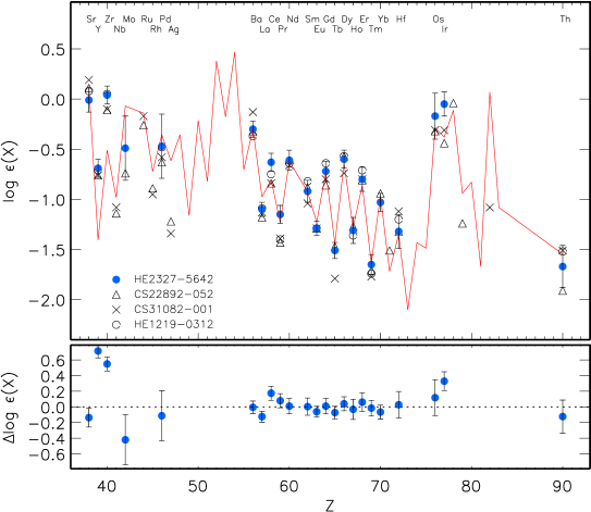
Figure 7: The heavy-element abundance pattern of HE 2327$-$5642 (filled circles) compared to the Solar system $r$-process (SSr) abundance pattern (continuous curve) scaled to match Ba–Hf. For comparison, the heavy element abundances of the benchmark r-II stars CS 22892-052 (open triangles), CS 31082-001 (crosses), and HE 1219-0312 (open circles) are shown. They have been normalized to the value derived for $\log\varepsilon_{\rm Eu}$ in HE 2327$-$5642. The bottom panel displays the difference between HE 2327$-$5642 and SSr defined as $\Delta\log\varepsilon(X)=\log\varepsilon_{\rm HE\,2327-5642}(X)-\log\varepsilon_{\rm SSr}(X)$.

Now we explore the abundance patterns of elements in the three $r$-process peaks.

4.4.2 The light trans-iron elements

Five elements with $38\leq Z\leq 46$ were measured in the region of the first peak. The only molybdenum line in the visible spectrum, Mo i 3864 Å, can be used to determine the element abundance of cool stars. In HE 2327$-$5642, this line is nearly free of blends, but it is weak: the central depth of the line is only $\sim 2$ % of the continuum. With $S/N\simeq 50$ of the observed spectrum in this wavelength region, the uncertainty of the derived Mo abundance was estimated to be $0.3$ dex.

A similar uncertainty is expected for palladium, which was detected in a single line, Pd i 3404 Å. In HE 2327$-$5642, this line is free of blends and is stronger compared to Mo i 3864 Å, but it is located in a spectral range where the $S/N$ is only 20 to 25.

Strontium is observed in HE 2327$-$5642 in two strong resonance lines, Sr ii 4077 and 4215 Å. Both lines are affected by HFS of the odd isotope ${}^{87}{\rm Sr}$. The synthetic spectrum was calculated with the ${}^{87}{\rm Sr}$ fraction of 0.22 corresponding to a pure $r$-process production of strontium (Arlandini et al., 1999, stellar model).

4.4.3 The second $r$-process peak elements

With 15 elements measured in the Ba–Hf range (see Fig. 8 for holmium and hafnium), the second $r$-process peak is the best-constrained one among the three peaks,

The barium abundance given in Table 5 was determined from the three subordinate lines, Ba ii 5853, 6141, and 6497 Å, which are nearly free of HFS effects. According to our estimate for Ba ii 6497 Å, neglecting HFS makes a difference in abundance of no more than 0.01 dex. In contrast, the Ba ii 4554 Å resonance line is strongly affected by HFS. The even isotopes are unaffected by HFS, while the odd isotopes show significant HFS, and thus the element abundance derived from this line depends on the Ba isotope mixture adopted in the calculations. Since the odd isotopes ${}^{135}{\rm Ba}$ and ${}^{137}{\rm Ba}$ have very similar HFS, the abundance is essentially dependent on the total fractional abundance of these odd isotopes, $f_{\mathrm{odd}}$. For example, using the Solar Ba isotope mixture with $f_{\mathrm{odd}}=0.18$, we obtained a $0.34$ dex larger abundance from Ba ii 4554 Å compared to the mean abundance of the subordinate lines. In the LTE calculations, the difference was reduced by $0.20$ dex when we adopted a pure $r$-process Ba isotope mixture with $f_{\mathrm{odd}}=0.46$, as predicted by Arlandini et al., (1999, stellar model). The remaining discrepancy between the resonance and subordinate lines has been largely removed by NLTE calculations. Thus, our analysis of HFS affecting the Ba ii 4554 Å resonance line suggests a pure $r$-process production of barium in HE 2327$-$5642.

The lines of Eu ii and Yb ii detected in HE 2327$-$5642 consist of multiple IS and HFS components. To derive the total abundance of the given element, we adopted in our calculations a pure $r$-process isotope mixture from the predictions of Arlandini et al., (1999, stellar model): ${}^{151}{\rm Eu}$ : ${}^{153}{\rm Eu}$ = 39 : 61 and ${}^{171}{\rm Yb}$ : ${}^{172}{\rm Yb}$ : ${}^{173}{\rm Yb}$ : ${}^{174}{\rm Yb}$ : ${}^{176}{\rm Yb}$ = 18.3 : 22.7 : 18.9 : 23.8 : 16.3. All the lines of Nd ii and Sm ii observed in HE 2327$-$5642 are rather weak, and they were treated as single lines.

There is only one hafnium line that can be measured in HE 2327$-$5642. The observed feature is attributed to a combination of the Hf ii 3399.79 Å and NH 3399.79 Å molecular line. With $\log gf=-1.358$ taken from Kurucz, (1993) and scaled down by $-0.3$ dex and the nitrogen abundance $\log\varepsilon_{\rm N}=4.78$, the molecular line contributes approximately 45 % to the 3399 Å blend (Fig. 8). Ignoring the molecular contaminant completely leads to a $0.17$ dex larger hafnium abundance. We therefore estimate the uncertainty of the obtained Hf abundance to be $0.15$ dex.

4.4.4 The heaviest elements

The third peak and actinides were probed for three elements, osmium, iridium, and thorium. The abundance of osmium was determined from a single line, Os i 4260 Å. The line is weak, with a center line depth of 2.5% of the continuum flux, and is nearly free of blends. With a high signal-to-noise ratio ($S/N\simeq 100$) of the observed spectrum, the uncertainty of the derived osmium abundance was estimated as 0.2 dex.

Figure 8: The best fits (continuous curve) of Ho ii 3456 Å (top panel) and Hf ii 3399 Å (bottom panel) in the observed spectrum of HE 2327$-$5642 (bold dots). The dashed curves show the effect of a 0.1 dex variation of the abundance on the synthetic spectrum. The dotted curves show the synthetic spectrum with no holmium and hafnium in the atmosphere.

Figure 9: The same as in Fig. 8, but for Ir i 3513 and 3800 Å.

Figure 10: The same as in Fig. 8, but for Th ii 4019 Å.

Two iridium lines, Ir i 3513 and 3800 Å, were clearly detected in HE 2327$-$5642 (Fig. 9). The theoretical profiles were calculated with taking HFS effect into account and iridium isotope abundance ratio ${}^{191}{\rm Ir}$:${}^{193}{\rm Ir}$ = 37 : 63, which is obtained to be the same for the Solar system matter (Lodders, 2003) and the matter produced in the $r$-process (Arlandini et al., 1999). The Ir i 3800 Å line was measured in two observed spectra, BLUE390 and 437BLUE, (Table 2) and seems reasonably reliable. With its equivalent width of 5.8 mÅ and $S/N\simeq 100$ of the observed spectrum, the uncertainty of the derived iridium abundance was estimated as 0.08 dex. The Ir i 3513 Å line served as a verification of that it agrees with the other line. The blend at 3513.6 Å is well fitted with $\log\varepsilon_{\rm Ir}=-0.05$ found from Ir i 3800 Å, as shown in Fig. 9.

The radioactive element thorium was clearly detected in HE 2327$-$5642 in the Th ii 4019 Å line (Fig. 10), but proved rather challenging for the determination of stellar age of HE 2327$-$5642. Unhappily, the observed spectrum around Th ii 4019 Å has low signal-to-noise ratio ($S/N\simeq 50$), and the uncertainty of the derived thorium abundance was estimated as 0.2 dex.

4.5 Error budget

We performed a detailed error analysis on HE 2327$-$5642, in order to estimate the uncertainties of the abundance measurements for the heavy elements beyond the iron group. Stochastic errors ($\sigma_{obs}$) arising from random uncertainties of the continuum placement, line profile fitting, and $gf$-values, are represented by a dispersion of the measurements of multiple lines around the mean ($\sigma_{\log\varepsilon}$), as given in Table 5 when $N\geq 2$ lines of an element are observed. Observational errors of the species with a single line used in abundance analysis were discussed in Sect. 4.4. Systematic uncertainties include those which exist in the adopted stellar parameters, in the used hydrostatic model atmospheres, and in the LTE line formation calculations. As argued in Sect. 4.4, the latter is not expected to influence the abundance pattern of the elements in the range from La to Th.

It is difficult to estimate the uncertainty introduced by using the 1D model atmosphere. The elements in the La–Th range, for example, are observed in the lines of their majority species. The detected lines arise from either the ground or low-excitation levels, and most of them are relatively weak; i.e., $W_{\lambda}<30$ mÅ. This means that they all are formed in the same atmospheric layers. It would therefore be rather unexpected if there were significantly different 3D effects for individual elements in the La–Th range. This is different from the case of the elements in the Sr–Pd range, Ba, and Yb, which are observed in either the strong lines (e.g. Sr ii 4215Å, Ba ii 6141Å, Yb ii 3694Å) or the lines of the minority species Mo i and Pd i. Both NLTE and 3D effects may have a strong influence on their derived abundance. Hence we examined here only those uncertainties linked to our choice of stellar parameters. These were estimated by varying $T_{\mbox{\scriptsize eff}}$ by $-70$ K, $\log g$ by $-0.1$ dex, and $\xi$ by $-0.1$ km s^-1 in the stellar atmosphere model.

Table 6: Error budget for neutron-capture elements in HE 2327$-$5642.

El.	$\Delta T$	$\Delta\log g$	$\Delta\xi$	$\Delta$	$\sigma_{obs}$	$\sigma_{tot}$
	$-70$ K	$-0.1$ dex	$-0.1$ km s-1	($T,g,\xi$)
(1)	(2)	(3)	(4)	(5)	(6)	(7)
Sr II	$-0.08$	$-0.01$	0.09	0.12	0.00	0.12
Y II	$-0.05$	$-0.03$	0.02	0.06	0.06	0.09
Zr II	$-0.06$	$-0.03$	0.02	0.07	0.05	0.09
Mo I	$-0.10$	$<0.01$	$<0.01$	0.10	0.3	0.32
Pd I	$-0.10$	$<0.01$	$<0.01$	0.10	0.3	0.32
Ba II	$-0.06$	$-0.03$	0.03	0.07	0.03	0.08
La II	$-0.06$	$-0.03$	$<0.01$	0.07	0.02	0.07
Ce II	$-0.06$	$-0.03$	$<0.01$	0.07	0.06	0.09
Pr II	$-0.06$	$-0.03$	$<0.01$	0.07	0.06	0.09
Nd II	$-0.06$	$-0.03$	0.01	0.07	0.08	0.10
Sm II	$-0.06$	$-0.03$	$<0.01$	0.07	0.09	0.11
Eu II	$-0.06$	$-0.03$	0.01	0.07	0.02	0.07
Gd II	$-0.06$	$-0.03$	0.01	0.07	0.07	0.10
Tb II	$-0.07$	$-0.03$	0.01	0.08	0.03	0.08
Dy II	$-0.06$	$-0.03$	0.03	0.07	0.06	0.09
Ho II	$-0.07$	$-0.03$	$<0.01$	0.08	0.10	0.13
Er II	$-0.07$	$-0.03$	$<0.01$	0.08	0.09	0.12
Tm II	$-0.06$	$-0.03$	0.01	0.07	0.08	0.10
Yb II	$-0.04$	$-0.03$	0.07	0.09	0.02	0.09
Hf II	$-0.07$	$-0.03$	0.01	0.08	0.15	0.17
Os I	$-0.11$	$<0.01$	$<0.01$	0.11	0.2	0.23
Ir I	$-0.09$	$-0.01$	$<0.01$	0.09	0.08	0.12
Th II	$-0.07$	$-0.03$	$<0.01$	0.08	0.2	0.21

Table 6 summarizes the various sources of uncertainties. The quantity $\Delta(T,g,\xi)$ listed in Col. 5 is the total impact of varying each of the three parameters, computed as the quadratic sum of Cols. 2, 3, and 4. The total uncertainty $\sigma_{tot}$ (Col. 7) of the absolute abundance of each element is computed by the quadratic sum of the stochastic ($\sigma_{obs}$) and systematic ($\Delta(T,g,\xi)$) errors.

5 Comparison to other r-II stars and Solar r-process abundances

The abundance pattern of the neutron-capture elements in the range from Sr to Os in HE 2327$-$5642 is very similar to that of other well-studied r-II stars. Figure 7 shows comparisons with CS 22892-052 (Sneden et al., 2003), CS 31082-001 (Hill et al., 2002; Plez et al., 2004), and HE 1219-0312 (Hayek et al., 2009). For example, the dispersion around the mean of the quantities $(\log\varepsilon_{\rm HE\,2327-5642}-\log\varepsilon_{\rm CS\,22892-052})$ amounts to $0.10$ dex, which is at the level of $1\sigma$ error bars in the abundance determinations of the individual elements.

Iridium in HE 2327$-$5642 seems to be overabundant with respect to CS 22892-052 and CS 31082-001. Roederer et al., (2009) compiled and/or revised the neutron-capture element abundances for a sample of $r$-process rich stars including CS 22892-052 and CS 31082-001, and they obtained a mean iridium to europium ratio of $\log(\mathrm{Ir}/\mathrm{Eu})=0.90\pm 0.09$ for 15 stars. For HE 2327$-$5642, we derived $\log(\mathrm{Ir}/\mathrm{Eu})=1.24$. We investigated possible sources of the difference between our analysis and that of Roederer et al., (2009), and found one which could at least partly explain it. The iridium abundances in the Roederer et al., (2009) study were underestimated by approximately 0.2 dex due to using the partition functions of Ir ii as implemented in the MOOG code (C. Sneden, private communication), which are about a factor of two lower compared to the ones we used in our study. We have compared the partition functions thoroughly and are satisfied that our new data, which are based on the best available energy level data, are more accurate. In all other relevant respects (i.e., $gf$-values, HFS data, ionization potential of Ir i), our data and methods and those of Roederer et al., (2009) are identical. The difference in the codes used for the abundance determination cannot play a role only for iridium, leaving all the other determinations unaffected. Hence, we are left with a discrepancy of 0.14 dex in $\log(\mathrm{Ir}/\mathrm{Eu})$ between HE 2327$-$5642 and the stellar sample of Roederer et al., (2009). However, in order to draw a firm conclusion on this point, the abundance determinations have to confirmed from better measurements and from new detections of the third $r$-process peak elements.

In Fig. 7, we also plot the Solar $r$-process residuals. The decomposition of the $s$- and $r$-process contributions is based on the meteoritic abundances of Lodders et al., (2009) and the $s$-process abundances of Arlandini et al., (1999, stellar model). The absolute $s$-process abundances were obtained by Arlandini et al., (1999) by normalization to the Solar abundance of the pure $s$-process isotope ${}^{150}{\rm Sm}$ taken from Anders & Grevesse, (1989). The difference in the Sm abundance between Anders & Grevesse, (1989) and Lodders et al., (2009) was taken into account. Hereafter, the Solar $r$-residuals are referred to as the Solar system $r$-process (SSr) abundance pattern.

The elements in the range from Ba to Hf in HE 2327$-$5642 were found to match the scaled Solar $r$-process pattern very well, with a dispersion of 0.07 dex around the mean of the differences $(\log\varepsilon_{\rm HE\,2327-5642}-\log\varepsilon_{\rm SSr})$. This is in line with earlier results obtained for other $r$-process rich stars, e.g. CS 22892-052 (Sneden et al., 2003), CS 31082-001 (Hill et al., 2002), HD 221170 (Ivans et al., 2006), CS 29491-069 and HE 1219-0312 (Hayek et al., 2009), and it gives further evidence for an universal production ratio of these elements during the Galaxy history. It is worth noting that the use of the partition function of Ho ii from Bord & Cowley, (2002) improves the comparison to the scaled Solar $r$-process for holmium.

For the lighter elements in HE 2327$-$5642, the difference $\Delta\log\varepsilon(X)=\log\varepsilon_{\rm obs}(X)-\log\varepsilon_{\rm SSr}(X)$ reveals a large spread of the data, between $-0.4$ dex (Mo) and $+0.7$ dex (Y). In the following we will show that at least a major fraction of the departures from the Solar $r$-process found for the light trans-iron elements is likely to be due to inaccurate Solar $r$-residuals.

For a given element, the $r$-residual is obtained by subtracting theoretical $s$-process yields from the observed total Solar abundance. Consider, e.g., the $s$-process abundances from Arlandini et al., (1999, stellar model) and use the Solar total abundances from two different sources, Lodders et al., (2009, meteoritic) and Asplund et al., (2009, photospheric). The 0.02 dex increase of the yttrium abundance as one changes from Lodders et al., (2009) to the Asplund et al., (2009) data leads to a 0.65 dex increase of the $r$-residual. A notable difference between two sets of the Solar $r$-process abundances was found for all elements with dominant $s$-process contribution to their Solar abundances; for example, $-0.58$ dex for Sr, $-0.40$ dex for Zr, $-0.31$ dex for La, etc. (see Fig. 11). This is because the calculation of the $r$-residuals involves the subtraction of a large number from another large number, so that any small variations of one of them leads to a dramatic change of the difference.

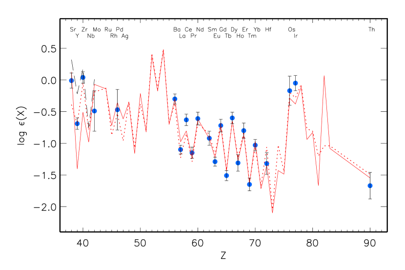
Figure 11: The heavy-element abundance pattern of HE 2327$-$5642 (filled circles) compared to the $r$-residuals calculated with various Solar total abundances and $s$-process abundances. Continuous and dotted curves correspond to the predicted $s$-process abundances of Arlandini et al., (1999, stellar model) and the Solar total abundances from Lodders et al., (2009) and Asplund et al., (2009), respectively. The dashed curve (only Sr–Mo) corresponds to the $s$-process abundances of Travaglio et al., (2004) and the Solar total abundances of Lodders et al., (2009). Each $r$-process abundance pattern was scaled to match the Ba–Hf in HE 2327$-$5642.

Significant uncertainties in the $r$-residual arise also from differences between $s$-process calculations. For example, Arlandini et al., (1999) obtained the $s$-process abundance distribution as a best-fit to the Solar main s-component using stellar AGB models of 1.5 $M_{\odot}$ and 3 $M_{\odot}$ with half-Solar metallicity. Travaglio et al., (1999, 2004) calculated the $s$-process contribution to the Solar abundances by integration of the $s$-process yields of different generations of AGB stars, i.e. considering the whole range of Galactic metallicities. In both studies, very similar results were found for Ba and Eu; however, Travaglio et al., (2004) predicted lower $s$-process abundances for the elements in the Sr–Mo range. Consequently, their Solar $r$-residuals were significantly increased, as shown in Fig. 11. From this discussion, it is clear that no solid conclusion can be drawn with respect to the existence of departures from the scaled Solar $r$-process pattern in the Sr–Pd region in r-II stars.

Observations of metal-poor halo stars give evidence for the existence of a distinct production mechanism for the light trans-iron (Sr–Zr) and heavy elements beyond Ba in the early Galaxy (Aoki et al., 2005; François et al., 2007; Mashonkina et al., 2007). We have chosen strontium and europium as representative elements of the first and second neutron-capture element peaks and inspected the Sr/Eu abundance ratios in a pre-selected sample of halo stars with a dominant contribution of the $r$-process to the production of heavy elements beyond Ba, i.e. with $\mathrm{[Ba/Eu]}\leq-0.4$. The stars are separable into three groups, depending on the observed europium enhancement. Nine r-II stars ($\mathrm{[Eu/Fe]}>1.0$) were taken from Hill et al., (2002); Sneden et al., (2003); Christlieb et al., (2004); Honda et al., (2004); Barklem et al., (2005); François et al., (2007); Lai et al., (2008); Hayek et al., (2009), 32 r-I stars ($0.2\geq\mathrm{[Eu/Fe]}<1.0$) from Cowan et al., (2002); Honda et al., (2004); Barklem et al., (2005); Ivans et al., (2006); François et al., (2007); Mashonkina et al., (2007); Lai et al., (2008); Hayek et al., (2009), and 12 stars with $\mathrm{[Eu/Fe]}\leq 0.06$ (hereafter Eu-poor stars) from Honda et al., (2004, 2006, 2007); Barklem et al., (2005); François et al., (2007).

As expected, each group of stars reveals very similar Ba/Eu abundance ratios, as shown in the bottom panel of Fig. 12, with mean Ba/Eu ratios of $\log(\mathrm{Ba}/\mathrm{Eu})=1.05\pm 0.10$ (r-II stars), $1.06\pm 0.13$ (r-I stars), and $1.14\pm 0.08$ (Eu-poor stars). Note that $\log(\mathrm{Ba}/\mathrm{Eu})_{r}=0.93$ for a pure $r-$process production of heavy elements (Arlandini et al., 1999). This suggests that only a small number of $s$-nuclei (including those of strontium) existed in the matter out of which these stars formed. The Sr/Eu abundance ratios reveal a clear separation between each of these three groups (Fig. 12). Note that the Zr/Eu ratios exhibit very similar behavior. The mean Zr/Eu abundance ratios are $\log(\mathrm{Zr}/\mathrm{Eu})=1.42\pm 0.19$ (r-II stars), $1.75\pm 0.15$ (r-I stars), and $2.30\pm 0.20$ (Eu-poor stars). HE 2327$-$5642, having $\log(\mathrm{Ba}/\mathrm{Eu})=1.01$, $\log(\mathrm{Sr}/\mathrm{Eu})=1.28$ (crossed circle in Fig. 12), and $\log(\mathrm{Zr}/\mathrm{Eu})=1.33$, clearly belongs to the group of r-II stars.

From Figs. 7 and 12, it is clear that the first and second $r$-process peak elements in the r-II stars are of common origin. However, the origin of the first neutron-capture peak elements in the r-I and Eu-poor stars is still unclear, despite of a number of studies (Truran et al., 2002; Travaglio et al., 2004; Farouqi et al., 2009).

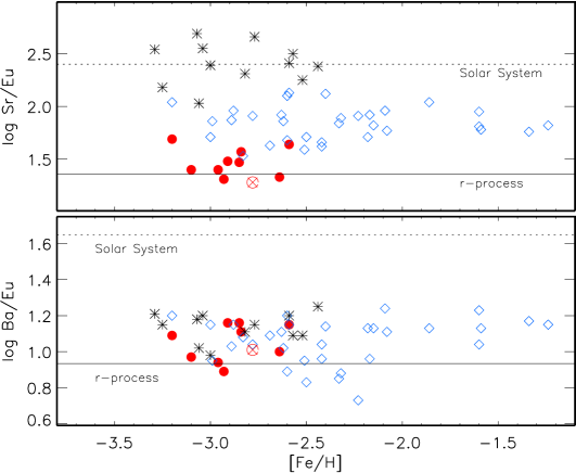
Figure 12: The Sr/Eu (top panel) and Ba/Eu (bottom panel) abundance ratios in r-II (filled circles), r-I (open rombs), and Eu-poor (asterisks) stars (for the sources of the data, see text). HE 2327$-$5642 is shown by a crossed open circle. The solid and dotted lines indicate the pure $r$-process and Solar system ratios, respectively.

6 Age determination

The detection of thorium permits a nucleo-chronometric age estimation of HE 2327$-$5642 by means of a comparison of the observed Th-to-stable neutron capture element abundance ratios with $\log$(Th/$X$)₀, the corresponding initial values at the time when the star was born:

$$\tau=46.7\,\mathrm{Gyr}\,\left[\log({\rm Th}/X)_{0}-\log({\rm Th}/X)_{obs}\right].$$

Considering the uncertainty of the thorium abundance of 0.2 dex, which translates into an age uncertainty of 9.3 Gyr, a precise age estimation is not possible. Nevertheless, we investigated how the results depend on the adopted values of $\log$(Th/$X$)₀, and which Th/$X$ pairs are possibly reliable chronometers. We assume that thorium was produced together with the lighter elements in the range between Ba and Hf.

We first determined the age of the star using the initial abundance ratios from the dynamical network calculations of Farouqi et al., (2008). They considered a core-collapse supernova (SN II) with an adiabatically expanding high-entropy wind (HEW) as the astrophysical environment for the $r$-process. In the HEW scenario, the total nucleosynthetic yield is the sum of SN ejecta with multiple components in different entropy ranges. Farouqi et al., (2008) found that heavy elements beyond $Z\simeq 52$ are produced in the highest entropy ($S>150$) zones in the so-called “main” $r$-process. The HEW model production ratios, $\mathrm{PR}=\log(\mathrm{Th}/X)_{0}$, as given by Hayek et al., (2009), and the calculated ages for multiple Th/$X$ pairs (where $X$ is one of the elements in the Ba–Ir range for which we determined an abundance) are listed in Table 7.

The age uncertainties introduced by the measurement uncertainties are listed in the column “Error”. They were calculated as $\sigma_{\tau}=46.7\,\sqrt{\sigma^{2}_{obs}(X)+\sigma^{2}_{obs}({\rm Th})}$ Gyr with $\sigma_{obs}$ from Table 6. Variations of the stellar parameters $T_{\mbox{\scriptsize eff}}$ and $\log g$ yielded an uncertainty of 1.5 Gyr in the final age. It can be seen that individual pairs reveal a large spread of stellar ages. The mean value is $\tau=15.1\pm 7.4$ Gyr. As noted by Hayek et al., (2009), the estimate for hafnium is bracketed for the HEW model due to problems with the nuclear data. Neglecting hafnium and also osmium in the view of its less reliable stellar abundance yields $\tau=13.3\pm 6.2$ Gyr, which agrees well with the expectation of the age of an extremely metal-poor star which formed in the early Galaxy. Note that the cosmic age derived from the results of the Wilkinson Microwave Anisotropy Probe (WMAP) experiment is $13.7\pm 0.2$ Gyr (Spergel et al., 2003).

For an additional estimate of the age of HE 2327$-$5642, we employed the Solar $r$-residual ratios $(\mathrm{Th}/X)_{0}$ for the elements for which the $r$-process fraction exceeds 70 % (columns SSr in Table 7). Since these are measured values, they depend only weakly on theoretial predictions and their associated nuclear physics uncertainties. Since the Sun is approximately 4.5 Gyr old, the corresponding correction accounting for the thorium radiative decay was introduced to the Solar current thorium abundance. The resulting mean age of HE 2327$-$5642, $\tau=7.4\pm 5.5$ Gyr, calculated using all stable elements from Sm to Ir seems low for a halo star. If we neglect the estimate based on Th/Ir, which is clearly an outlier (i.e., $\tau=21.0$ Gyr), we come to even lower stellar age of $\tau=5.9\pm 2.8$ Gyr.

Note that the stochastic error of the stellar age based on the HEW model predictions is large compared to that for the Solar $r$-residual ratios. This is most likely due to the uncertainty of the theoretical yields for individual elements.

Table 7: Logarithmic production ratios (PR) for the HEW model and Solar system $r$-process (SSr) and corresponding radioactive decay ages in HE 2327$-$5642.

Element	Stellar	HEW $S=10\dots 300$			SSr
pair	ratio	PR	age,	Error,	PR	age,
			Gyr	Gyr		Gyr
Th/Ba	$-1.37$	$-0.96$	19.1	9.4
Th/La	$-0.57$	$-0.22$	16.3	9.4
Th/Ce	$-1.04$	$-0.62$	19.6	9.8
Th/Pr	$-0.52$	$-0.20$	14.9	9.8
Th/Nd	$-1.06$	$-0.87$	8.9	10.0
Th/Sm	$-0.75$	$-0.71$	1.9	10.2	$-0.62$	6.1
Th/Eu	$-0.38$	$-0.32$	2.8	9.4	$-0.32$	2.8
Th/Gd	$-0.95$	$-0.73$	10.3	9.9	$-0.82$	6.1
Th/Tb	$-0.16$				$-0.11$	2.3
Th/Dy	$-1.07$	$-0.69$	17.7	9.8	$-0.91$	7.5
Th/Ho	$-0.36$	$0.04$	18.7	10.4	$-0.27$	4.2
Th/Er	$-0.87$	$-0.48$	18.2	10.2	$-0.69$	8.4
Th/Tm	$-0.02$	$0.22$	11.2	10.0	$0.08$	4.7
Th/Hf	$-0.35$	$0.20$	25.7	11.7
Th/Os	$-1.50$	$-0.93$	26.6	13.2	$-1.26$	11.2
Th/Ir	$-1.62$			10.1	$-1.17$	21.0
mean(Ba–Ir)			15.1$\pm$7.4		7.4$\pm$5.5
final			13.3$\pm$6.2		5.9$\pm$2.8
			(Ba–Tm)		(Sm–Os)

7 Conclusions

The high-quality VLT/UVES spectra of HE 2327$-$5642 enabled the determination of accurate abundances for 40 elements, including 23 elements in the nuclear charge range between $Z=38$–$90$. We confirmed that HE 2327$-$5642 is strongly $r$-process enhanced, having $[r/\mathrm{Fe}]=0.99\pm 0.03$ where $r$ denotes the average of the abundances of seven elements (i.e., Eu, Gd, Tb, Dy, Ho, Er, and Tm), with an $r$-process contribution to the Solar system matter of more than 85 % according to the $r$-residuals of Arlandini et al., (1999). HE 2327$-$5642 and three benchmark r-II stars, CS 22892-052 (Sneden et al., 2003), CS 31082-001 (Hill et al., 2002), and HE 1219-0312 (Hayek et al., 2009), have very similar abundance patterns of the elements in the range from Sr to Os. Hence, HE 2327$-$5642 is a member of the small sample of currently- known r-II stars.

The elements in the range from Ba to Hf in HE 2327$-$5642 match the scaled Solar $r$-process pattern very well. We showed that the Solar $r$-residuals for the first $r$-process peak elements are rather uncertain. They may vary as much as 0.5 dex or even more, depending on the adopted Solar total abundances and $s$-process fractions. Therefore, no firm conclusion can be drawn with respect to a relation of the light trans-iron elements in HE 2327$-$5642 and other r-II stars to the Solar $r$-process.

We found a clear distinction in Sr/Eu abundance ratios between the halo stars with different europium enhancement and suggest using the [Sr/Eu] ratio in addition to [Eu/Fe] to separate the strongly $r$-process enhanced (r-II) stars from the other halo stars with dominant contribution of the $r$-process to heavy element production. The r-II stars, whose stellar matter presumably has experienced a single nucleosynthesis event, have $\mathrm{[Eu/Fe]}>1\pm 0.1$, $\mathrm{[Ba/Eu]}=-0.60\pm 0.10$, and a low Sr/Eu abundance ratio of $\mathrm{[Sr/Eu]}=-0.92\pm 0.13$. Stars with very similar Ba/Eu ratios have two times (0.36 dex) larger Sr/Eu ratios if their Eu/Fe ratio is in the range $1.0<\mathrm{[Eu/Fe]}<0.2$ (i.e., r-I stars), and nearly an order of magnitude (0.93 dex) higher Sr/Eu ratios if $\mathrm{[Eu/Fe]}<0$ (Eu-poor stars). The origin of the first neutron-capture peak elements in the r-I stars and Eu-poor stars is still unclear. Further theoretical studies will be needed to elucidate this problem.

Only two elements, Os and Ir, of the third $r$-process peak were detected in HE 2327$-$5642. Iridium appears to be overabundant compared to the Ir abundance determined in other $r$-process enhanced stars. However, due to the uncertainty of the Ir abundance we cannot yet draw a firm conclusion on this point.

The detection of thorium permitted an estimate of the radioactive decay age of HE 2327$-$5642, although the age uncertainty of 9.3 Gyr introduced by the uncertainty of the thorium abundance is rather large. Employing multiple Th/$X$ chronometers and initial production ratios based on the Solar $r$-residuals, an age of $5.9\pm 2.8$ Gyr was obtained from nine Th/$X$ pairs, involving elements in the Sm–Os range. Using the predictions of the HEW $r$-process model, as given by Hayek et al., (2009), we obtained $\tau=13.3\pm 6.2$ Gyr from 12 Th/$X$ pairs.

Based on our high-resolution spectra, covering $\sim 4.3$ years, we suspect that HE 2327$-$5642 is radial-velocity variable with a highly elliptical orbit of the system. Determination of the orbital period would provide the unique opportunity to determine a lower limit for the mass of the secondary in this system. Scenarios for the site of the $r-$process include a high-entropy wind from a type-II supernova (e.g. Woosley et al., 1994; Takahashi et al., 1994), ejecta from neutron star mergers (e.g. Freiburghaus et al., 1999), or the neutrino-driven wind of a neutron star newly-formed in an accretion induced collapse (AIC) event (e.g. Woosley & Baron, 1992; Qian & Wasserburg, 2003). According to these scenarios, it is expected that the secondary is a neutron-star. With a lower limit for the mass of the secondary it might be possible to constrain a scenario, because in the AIC case the neutron star is expected to have a mass just slightly above the Chandrasekhar mass, while core-collapse supernovae or neutron star mergers would result in remants of significantly higher mass.

Table 8: Line data and abundances from an analysis of HE 2327$-$5642. $\Gamma_{6}$ corresponds to 10 000 K. Column 6 gives references to the adopted $gf-$values. Column 13 gives references to the sources of the used IS and HFS data and adopted $\Gamma_{6}-$values.

Z	Atom/	$\lambda$	$E_{exc}$	$\log gf$	Ref	$\log\varepsilon$			[X/Fe]	$W_{\lambda}$	$\log\Gamma_{6}/N_{\rm H}$	Note, Ref.
	mol	(Å)	(eV)			Solar	LTE	NLTE		(mÅ)	(rad/s$\cdot$cm3)
1	2	3	4	5	6	7	8	9	10	11	12	13
3	Li 1	6707.80	0.00	0.167	NIST8	1.10	0.99		2.67	Syn	-7.574	IS:SRE95
												$\Gamma_{6}$:ABO
6	CH	4310.0 - 4312.5			BCB05	8.39	5.74		0.13	Syn
6	CH	4313.4 - 4313.8			BCB05	8.39	5.74		0.13	Syn
6	CH	4362.4 - 4364.6			BCB05	8.39	5.76		0.15	Syn
6	CH	4366.0 - 4367.0			BCB05	8.39	5.73		0.12	Syn
7	NH	3358 - 3361			K94	7.86	4.78		-0.30	Syn
11	Na 1	5889.96	0.00	0.110	NIST8	6.30	3.28	2.89	-0.63	Syn	-7.712	$\Gamma_{6}$:GLS04
11	Na 1	5895.93	0.00	-0.190	NIST8	6.30	3.24	2.96	-0.56	Syn	-7.712	the same
12	Mg 1	4571.10	0.00	-5.620	NIST8	7.54	4.86	4.98	0.22	Syn	-7.856	$\Gamma_{6}$:GLS04
12	Mg 1	4702.99	4.33	-0.440	NIST8	7.54	4.79	4.90	0.14	Syn	-6.956	the same
12	Mg 1	5528.41	4.33	-0.498	NIST8	7.54	4.84	4.96	0.20	Syn	-7.152	the same
13	Al 1	3961.52	0.01	-0.340	NIST8	6.47	2.50	3.02	-0.67	Syn	-7.552	$\Gamma_{6}$:GLS04
14	Si 1	3905.53	1.91	-1.041	BL91	7.52	4.85		0.11	Syn	-7.440	$\Gamma_{6}$:ABO
20	Ca 1	4425.44	1.88	-0.358	SON75	6.33	3.52	3.76	0.20	23.7	-7.432	$\Gamma_{6}$:MKP07
20	Ca 1	5349.46	2.71	-0.310	SR81	6.33	3.52	3.78	0.21	4.6	-7.652	$\Gamma_{6}$:S81
20	Ca 1	5588.75	2.53	0.358	SR81	6.33	3.57	3.86	0.26	22.8	-7.628	$\Gamma_{6}$:S81
20	Ca 1	5857.45	2.93	0.240	SR81	6.33	3.67	3.86	0.36	11.2	-7.316	$\Gamma_{6}$:S81
20	Ca 1	6122.22	1.89	-0.315	SON75	6.33	3.68	3.90	0.36	29.5	-7.189	$\Gamma_{6}$:ABO
20	Ca 1	6162.17	1.90	-0.089	SON75	6.33	3.63	3.84	0.32	38.6	-7.189	$\Gamma_{6}$:ABO
20	Ca 1	6169.56	2.53	-0.478	SR81	6.33	3.52	3.81	0.21	4.7	-7.264	$\Gamma_{6}$:S81
20	Ca 1	6439.08	2.53	0.390	SR81	6.33	3.63	3.80	0.31	27.4	-7.704	$\Gamma_{6}$:S81
20	Ca 2	8498.02	1.69	-1.416	Th89	6.33	-	3.82	0.27	Syn	-7.676	IS:NBI98
												$\Gamma_{6}$:ABO
21	Sc 2	4246.82	0.32	0.240	LD89	3.10	0.08		-0.24	Syn		HFS:MPS95
21	Sc 2	4400.39	0.60	-0.540	LD89	3.10	0.08		-0.24	Syn		the same
21	Sc 2	4415.56	0.60	-0.670	LD89	3.10	0.13		-0.19	Syn		the same
21	Sc 2	5031.02	1.36	-0.400	LD89	3.10	0.09		-0.23	Syn		the same
22	Ti 1	3998.64	0.05	-0.056	WF75	4.90	2.14		0.02	37.3	-7.654	$\Gamma_{6}$:ABO
22	Ti 1	4533.25	0.85	0.476	WF75	4.90	2.06		-0.06	19.7	-7.593	the same
22	Ti 1	4534.78	0.84	0.280	WF75	4.90	2.01		-0.11	12.5	-7.596	the same
22	Ti 1	4981.73	0.85	0.504	WF75	4.90	2.15		0.03	25.6	-7.626	the same
22	Ti 1	4991.06	0.84	0.380	WF75	4.90	2.15		0.03	21.0	-7.629	the same
22	Ti 1	5022.87	0.83	-0.434	WF75	4.90	2.14		0.02	3.9	-7.633	the same
22	Ti 1	5024.85	0.82	-0.602	WF75	4.90	2.32		0.20	4.1	-7.635	the same
22	Ti 1	5039.96	0.02	-1.130	WF75	4.90	2.09		-0.03	5.7	-7.720	the same
22	Ti 1	5064.66	0.05	-0.991	WF75	4.90	2.18		0.06	8.8	-7.719	the same
22	Ti 1	5210.39	0.05	-0.884	WF75	4.90	2.21		0.09	11.8	-7.724	the same
22	Ti 2	3913.47	1.12	-0.420	PTP01	4.90	2.29		0.17	87.4
22	Ti 2	4028.34	1.89	-0.960	PTP01	4.90	2.25		0.13	21.8
22	Ti 2	4053.83	1.89	-1.130	PTP01	4.90	2.11		-0.01	11.9
22	Ti 2	4290.22	1.16	-0.850	PTP01	4.90	2.16		0.04	66.5
22	Ti 2	4300.05	1.18	-0.440	PTP01	4.90	2.41		0.29	93.3
22	Ti 2	4394.05	1.22	-1.780	PTP01	4.90	2.24		0.12	20.5
22	Ti 2	4395.03	1.08	-0.540	PTP01	4.90	2.22		0.10	88.0
22	Ti 2	4395.85	1.24	-1.930	PTP01	4.90	2.29		0.17	16.2
22	Ti 2	4399.77	1.24	-1.190	PTP01	4.90	2.29		0.17	51.4
22	Ti 2	4417.72	1.16	-1.190	PTP01	4.90	2.23		0.11	53.0
22	Ti 2	4418.33	1.24	-1.970	PTP01	4.90	2.23		0.11	13.3
22	Ti 2	4443.79	1.08	-0.720	PTP01	4.90	2.22		0.10	79.9
22	Ti 2	4444.56	1.12	-2.240	PTP01	4.90	2.29		0.17	11.7
22	Ti 2	4450.48	1.08	-1.520	PTP01	4.90	2.24		0.12	40.2
22	Ti 2	4464.45	1.16	-1.810	PTP01	4.90	2.33		0.21	26.0
22	Ti 2	4468.51	1.13	-0.600	BHN93	4.90	2.20		0.08	81.8
22	Ti 2	4470.86	1.16	-2.020	PTP01	4.90	2.07		-0.05	10.6
22	Ti 2	4501.27	1.12	-0.770	PTP01	4.90	2.23		0.11	77.5
22	Ti 2	4533.97	1.24	-0.530	PTP01	4.90	2.10		-0.02	76.0
22	Ti 2	4563.76	1.22	-0.690	PTP01	4.90	2.05		-0.07	67.7
22	Ti 2	4571.97	1.57	-0.320	PTP01	4.90	2.08		-0.04	67.7
22	Ti 2	5185.91	1.89	-1.490	PTP01	4.90	2.14		0.02	7.3
22	Ti 2	5188.70	1.58	-1.050	PTP01	4.90	2.20		0.08	36.4
22	Ti 2	5226.55	1.57	-1.260	PTP01	4.90	2.21		0.09	26.9
22	Ti 2	5336.79	1.58	-1.590	PTP01	4.90	2.20		0.08	14.3
22	Ti 2	5381.01	1.57	-1.920	PTP01	4.90	2.15		0.03	6.6
23	V 2	3530.76	1.07	-0.600	FW96	4.00	0.84		-0.38	Syn
23	V 2	3545.19	1.10	-0.390	FW96	4.00	0.84		-0.38	Syn
23	V 2	3592.03	1.10	-0.370	FW96	4.00	0.88		-0.34	Syn
23	V 2	4005.71	1.82	-0.460	FW96	4.00	1.01		-0.21	Syn
24	Cr 1	4254.33	0.00	-0.114	MFW88	5.64	2.22		-0.64	80.4	-7.675	$\Gamma_{6}$:ABO
24	Cr 1	4274.80	0.00	-0.230	MFW88	5.64	2.16		-0.70	73.9	-7.675	the same
24	Cr 1	5206.04	0.94	0.019	MFW88	5.64	2.31		-0.55	45.1	-7.597	the same
24	Cr 1	5345.81	1.00	-0.980	MFW88	5.64	2.43		-0.43	8.7	-7.620	the same
24	Cr 1	5348.33	1.00	-1.290	FW96	5.64	2.34		-0.52	3.6	-7.620	the same
24	Cr 1	5409.80	1.03	-0.720	MFW88	5.64	2.44		-0.42	14.1	-7.620	the same
25	Mn 1	4030.75	0.00	-0.470	BBP84	5.37	1.53		-1.06	Syn	-7.552	HFS:LGB03
												$\Gamma_{6}$:ABO
25	Mn 1	4033.06	0.00	-0.620	BBP84	5.37	1.53		-1.06	Syn	-7.552	the same
25	Mn 1	4034.48	0.00	-0.810	BBP84	5.37	1.53		-1.06	Syn	-7.552	the same
25	Mn 1	4041.35	2.11	0.280	BBP84	5.37	1.89		-0.70	Syn	-7.701	$\Gamma_{6}$:ABO
25	Mn 2	3460.31	1.81	-0.640	KG00	5.37	1.91		-0.68	Syn		HFS:HSR99
25	Mn 2	3482.90	1.83	-0.840	KG00	5.37	1.94		-0.65	Syn		HFS:HSR99
25	Mn 2	3488.67	1.85	-0.950	KG00	5.37	2.10		-0.49	Syn		HFS:HSR99
26	Fe 1	3917.18	0.99	-2.155	OWL91	7.45	4.61	4.69	0.02	65.3	-7.695	$\Gamma_{6}$:ABO
26	Fe 1	3949.95	2.18	-1.251	OWL91	7.45	4.39	4.47	-0.19	36.8	-7.820	the same
26	Fe 1	4005.24	1.56	-0.580	OWL91	7.45	4.66	4.72	0.07	96.1	-7.620	the same
26	Fe 1	4132.06	1.61	-0.675	OWL91	7.45	4.61	4.68	0.02	94.3	-7.620	the same
26	Fe 1	4132.90	2.85	-1.006	OWL91	7.45	4.53	4.61	-0.06	19.4	-7.659	the same
26	Fe 1	4143.87	1.56	-0.511	OWL91	7.45	4.53	4.59	-0.06	98.0	-7.636	the same
26	Fe 1	4147.67	1.49	-2.074	OWL91	7.45	4.68	4.76	0.10	40.3	-7.648	the same
26	Fe 1	4202.03	1.49	-0.708	FMW88	7.45	4.64	4.67	0.05	98.4	-7.648	the same
26	Fe 1	4216.18	0.00	-3.356	FMW88	7.45	4.66	4.75	0.08	69.5	-7.797	the same
26	Fe 1	4250.79	1.56	-0.714	OWL91	7.45	4.69	4.73	0.10	95.9	-7.648	the same
26	Fe 1	4260.47	2.40	0.080	OWL91	7.45	4.45	4.51	-0.14	86.1	-7.274	the same
26	Fe 1	4415.12	1.61	-0.615	FMW88	7.45	4.56	4.61	-0.02	99.0	-7.652	the same
26	Fe 1	4427.31	0.05	-2.924	OWL91	7.45	4.77	4.86	0.18	87.6	-7.813	the same
26	Fe 1	4602.94	1.49	-2.209	OWL91	7.45	4.55	4.63	-0.04	36.3	-7.790	the same
26	Fe 1	4647.43	2.95	-1.351	OWL91	7.45	4.49	4.57	-0.10	7.9	-7.685	the same
26	Fe 1	4966.09	3.33	-0.871	OWL91	7.45	4.59	4.69	0.00	11.4	-7.218	the same
26	Fe 1	4994.13	0.92	-2.970	OWL91	7.45	4.63	4.72	0.04	31.4	-7.744	the same
26	Fe 1	5001.86	3.88	0.010	FMW88	7.45	4.57	4.67	-0.02	13.9	-7.273	the same
26	Fe 1	5014.94	3.94	-0.303	OWL91	7.45	4.59	4.68	0.00	8.7	-7.268	$\Gamma_{6}$:ABO
26	Fe 1	5051.63	0.92	-2.765	OWL91	7.45	4.71	4.80	0.12	48.0	-7.746	the same
26	Fe 1	5068.77	2.94	-1.042	OWL91	7.45	4.56	4.65	-0.03	14.1	-7.265	the same
26	Fe 1	5150.84	0.99	-3.040	OWL91	7.45	4.67	4.75	0.08	23.0	-7.742	the same
26	Fe 1	5166.28	0.00	-4.200	OWL91	7.45	4.69	4.78	0.10	33.5	-7.826	the same
26	Fe 1	5171.60	1.49	-1.720	OWL91	7.45	4.81	4.89	0.22	63.8	-7.687	the same
26	Fe 1	5192.34	3.00	-0.421	OWL91	7.45	4.53	4.61	-0.06	34.7	-7.266	the same
26	Fe 1	5194.94	1.56	-2.020	OWL91	7.45	4.67	4.75	0.08	41.0	-7.680	the same
26	Fe 1	5216.27	1.61	-2.080	OWL91	7.45	4.69	4.77	0.10	37.3	-7.674	the same
26	Fe 1	5281.79	3.04	-0.830	OWL91	7.45	4.65	4.73	0.06	18.4	-7.266	the same
26	Fe 1	5283.62	3.24	-0.520	OWL91	7.45	4.48	4.57	-0.11	21.8	-7.221	the same
26	Fe 1	5324.18	3.21	-0.100	BKK91	7.45	4.35	4.44	-0.24	35.1	-7.235	the same
26	Fe 1	5339.93	3.27	-0.720	OWL91	7.45	4.48	4.57	-0.11	14.5	-7.221	the same
26	Fe 1	5364.87	4.45	0.228	OWL91	7.45	4.47	4.58	-0.12	5.3	-7.136	the same
26	Fe 1	5367.47	4.41	0.440	OWL91	7.45	4.56	4.67	-0.03	8.9	-7.153	the same
26	Fe 1	5369.96	4.37	0.536	OWL91	7.45	4.58	4.69	-0.01	12.3	-7.179	the same
26	Fe 1	5383.37	4.31	0.645	OWL91	7.45	4.57	4.69	-0.02	16.8	-7.219	the same
26	Fe 1	5393.17	3.24	-0.720	BKK91	7.45	4.56	4.64	-0.03	15.2	-7.235	the same
26	Fe 1	5410.91	4.47	0.398	OWL91	7.45	4.62	4.73	0.03	7.5	-7.132	the same
26	Fe 1	5415.20	4.39	0.642	OWL91	7.45	4.52	4.63	-0.07	13.4	-7.182	the same
26	Fe 1	5434.52	1.01	-2.130	OWL91	7.45	4.77	4.85	0.18	80.4	-7.749	the same
26	Fe 1	5445.04	4.39	-0.020	FMW88	7.45	4.58	4.69	-0.01	5.7	-7.189	the same
26	Fe 1	5506.78	0.99	-2.797	OWL91	7.45	4.70	4.79	0.11	44.6	-7.753	the same
26	Fe 1	5586.76	3.37	-0.100	BKK91	7.45	4.42	4.51	-0.17	29.4	-7.221	the same
26	Fe 1	5615.64	3.33	0.050	BKK91	7.45	4.41	4.50	-0.18	37.2	-7.234	the same
26	Fe 1	6136.62	2.45	-1.410	OWL91	7.45	4.50	4.58	-0.09	25.2	-7.609	the same
26	Fe 1	6137.69	2.59	-1.350	OWL91	7.45	4.46	4.54	-0.13	19.1	-7.589	the same
26	Fe 1	6191.56	2.43	-1.417	OWL91	7.45	4.55	4.63	-0.04	24.4	-7.615	the same
26	Fe 1	6393.60	2.43	-1.570	OWL91	7.45	4.44	4.52	-0.14	20.0	-7.622	the same
26	Fe 1	6400.00	3.60	-0.290	BKK91	7.45	4.46	4.55	-0.13	14.0	-7.232	the same
26	Fe 1	6430.85	2.18	-1.950	OWL91	7.45	4.63	4.71	0.04	18.0	-7.704	the same
26	Fe 2	4508.29	2.86	-2.440	MB09	7.45	4.64	4.64	-0.03	22.6	-7.870	the same
26	Fe 2	4515.34	2.84	-2.600	MB09	7.45	4.81	4.81	0.14	21.2	-7.880	the same
26	Fe 2	4520.22	2.81	-2.650	MB09	7.45	4.61	4.61	-0.06	17.6	-7.880	the same
26	Fe 2	4923.93	2.89	-1.260	MB09	7.45	4.59	4.58	-0.07	68.5	-7.890	the same
26	Fe 2	5018.44	2.89	-1.100	MB09	7.45	4.64	4.63	-0.02	77.9	-7.890	the same
26	Fe 2	5197.58	3.23	-2.220	MB09	7.45	4.69	4.69	0.03	14.6	-7.880	the same
26	Fe 2	5234.62	3.22	-2.180	MB09	7.45	4.70	4.70	0.03	17.6	-7.880	the same
26	Fe 2	5284.11	2.89	-3.110	MB09	7.45	4.73	4.73	0.06	5.6	-7.890	the same
27	Co 1	3412.33	0.51	0.030	CSS82	4.92	1.87		-0.27	Syn	-7.666	HFS:P96
												$\Gamma_{6}$:ABO
27	Co 1	3417.16	0.58	-0.470	CSS82	4.92	1.97		-0.17	Syn	-7.657	$\Gamma_{6}$:ABO
27	Co 1	3489.40	0.92	0.150	CSS82	4.92	1.86		-0.28	Syn	-7.610	HFS:P96
												$\Gamma_{6}$:ABO
27	Co 1	3894.07	1.05	0.090	NKW99	4.92	1.98		-0.16	Syn	-7.648	HFS:P96
												$\Gamma_{6}$:ABO
27	Co 1	4118.77	1.05	-0.470	NKW99	4.92	2.05		-0.09	Syn	-7.710	$\Gamma_{6}$:ABO
27	Co 1	4121.31	0.92	-0.300	NKW99	4.92	2.05		-0.09	Syn	-7.724	HFS:P96
												$\Gamma_{6}$:ABO
28	Ni 1	3413.47	0.16	-1.480	HS80	6.23	3.18		-0.27	Syn	-7.690	$\Gamma_{6}$:ABO
28	Ni 1	3413.93	0.11	-1.720	FMW88	6.23	3.26		-0.19	Syn	-7.785	the same
28	Ni 1	3519.76	0.28	-1.420	BBP89	6.23	3.08		-0.37	Syn	-7.689	the same
28	Ni 1	3783.52	0.42	-1.310	HS80	6.23	3.00		-0.45	Syn	-7.780	the same
28	Ni 1	3807.14	0.42	-1.220	BBP89	6.23	3.00		-0.45	Syn	-7.694	the same
28	Ni 1	3858.29	0.42	-0.950	BBP89	6.23	2.98		-0.47	Syn	-7.700	the same
28	Ni 1	5035.37	3.63	0.290	WL97a	6.23	3.09		-0.36	Syn	-7.231	$\Gamma_{6}$:ABO
28	Ni 1	5476.90	1.83	-0.890	FMW88	6.23	3.20		-0.25	Syn
30	Zn 1	4722.16	4.01	-0.390	BG80	4.62	1.82		-0.02	Syn
30	Zn 1	4810.54	4.06	-0.170	BG80	4.62	1.84		0.00	Syn
38	Sr 2	4077.72	0.00	0.150	RCW80	2.92	-0.01	-0.16	-0.30	Syn	-7.792	HFS:BBH83
												$\Gamma_{6}$:MZG08
38	Sr 2	4215.54	0.00	-0.170	RCW80	2.92	-0.01	-0.16	-0.30	Syn	-7.792	the same
39	Y 2	3549.01	0.13	-0.280	HLG82	2.21	-0.74		-0.17	Syn
39	Y 2	3600.74	0.18	0.280	HLG82	2.21	-0.67		-0.10	Syn
39	Y 2	3611.04	0.13	0.010	HLG82	2.21	-0.73		-0.16	Syn
39	Y 2	3774.33	0.13	0.210	HLG82	2.21	-0.67		-0.10	Syn
39	Y 2	3788.69	0.10	-0.070	HLG82	2.21	-0.66		-0.09	Syn
39	Y 2	3950.35	0.10	-0.490	HLG82	2.21	-0.56		0.01	Syn
39	Y 2	4883.68	1.08	0.070	HLG82	2.21	-0.66		-0.09	Syn
39	Y 2	5087.43	1.08	-0.170	HLG82	2.21	-0.75		-0.18	Syn
39	Y 2	5205.73	1.03	-0.340	HLG82	2.21	-0.75		-0.18	Syn
40	Zr 2	3404.83	0.36	-0.490	LNA06	2.58	-0.01	0.07	0.26	Syn
40	Zr 2	3430.53	0.47	-0.160	LNA06	2.58	-0.03	0.08	0.28	Syn
40	Zr 2	3457.56	0.56	-0.470	MBM06	2.58	0.06	0.14	0.34	Syn
40	Zr 2	3479.39	0.71	-0.180	LNA06	2.58	0.02	0.16	0.36	Syn
40	Zr 2	3499.57	0.41	-1.060	LNA06	2.58	-0.02	0.02	0.22	Syn
40	Zr 2	3505.67	0.16	-0.390	LNA06	2.58	-0.02	0.03	0.23	Syn
40	Zr 2	3551.95	0.09	-0.360	LNA06	2.58	0.01	0.07	0.27	Syn
40	Zr 2	3573.08	0.32	-0.910	MBM06	2.58	0.09	0.18	0.38	Syn
40	Zr 2	3766.82	0.41	-0.830	LNA06	2.58	0.12	0.16	0.36	Syn
40	Zr 2	3998.97	0.56	-0.520	LNA06	2.58	0.07	0.15	0.35	Syn
40	Zr 2	4161.21	0.71	-0.590	LNA06	2.58	0.08	0.16	0.36	Syn
40	Zr 2	4208.98	0.71	-0.510	LNA06	2.58	0.07	0.15	0.35	Syn
42	Mo 1	3864.11	0.00	-0.010	FW96	1.92	-0.49		0.37	Syn
46	Pd 1	3404.58	0.81	0.330	XSD06	1.66	-0.72		0.40	Syn
56	Ba 2	4554.03	0.00	0.167	RCW80	2.17	-0.16	-0.25	0.36	Syn	-7.732	HFS:M98
												$\Gamma_{6}$:MZG08
56	Ba 2	5853.67	0.60	-1.000	RCW80	2.17	-0.29	-0.23	0.38	Syn	-7.584	$\Gamma_{6}$:ABO
56	Ba 2	6141.71	0.70	-0.076	RCW80	2.17	-0.34	-0.36	0.25	Syn	-7.584	$\Gamma_{6}$:ABO
56	Ba 2	6496.90	0.60	-0.377	RCW80	2.17	-0.28	-0.32	0.29	Syn	-7.584	$\Gamma_{6}$:ABO
57	La 2	3849.01	0.00	-0.450	LBS01	1.14	-1.11		0.53	Syn		HFS:LBS01
57	La 2	3949.10	0.40	0.490	LBS01	1.14	-1.13		0.51	Syn		HFS:LBS01
57	La 2	3988.51	0.40	0.210	LBS01	1.14	-1.13		0.51	Syn		HFS:LBS01
57	La 2	3995.74	0.17	-0.060	LBS01	1.14	-1.09		0.55	Syn		HFS:LBS01
57	La 2	4077.34	0.24	-0.060	LBS01	1.14	-1.11		0.53	Syn		HFS:LBS01
57	La 2	4086.71	0.00	-0.070	LBS01	1.14	-1.06		0.58	Syn		HFS:LBS01
57	La 2	4196.55	0.32	-0.300	LBS01	1.14	-1.11		0.53	Syn		HFS:LBS01
57	La 2	4920.98	0.13	-0.580	LBS01	1.14	-1.08		0.56	Syn		HFS:LBS01
58	Ce 2	3942.15	0.00	-0.220	LSC09	1.61	-0.60		0.57	Syn
58	Ce 2	3992.38	0.45	-0.220	LSC09	1.61	-0.57		0.60	Syn
58	Ce 2	3993.82	0.91	0.290	LSC09	1.61	-0.59		0.58	Syn
58	Ce 2	3999.24	0.30	0.060	LSC09	1.61	-0.67		0.50	Syn
58	Ce 2	4073.47	0.48	0.210	LSC09	1.61	-0.69		0.48	Syn
58	Ce 2	4075.70	0.70	0.230	LSC09	1.61	-0.68		0.49	Syn
58	Ce 2	4083.22	0.70	0.270	LSC09	1.61	-0.58		0.59	Syn
58	Ce 2	4127.36	0.68	0.310	LSC09	1.61	-0.70		0.47	Syn
58	Ce 2	4137.64	0.52	0.400	LSC09	1.61	-0.55		0.62	Syn
58	Ce 2	4222.60	0.12	-0.150	LSC09	1.61	-0.59		0.58	Syn
58	Ce 2	4562.36	0.48	0.210	LSC09	1.61	-0.68		0.49	Syn
58	Ce 2	4628.16	0.52	0.140	LSC09	1.61	-0.63		0.54	Syn
59	Pr 2	4143.12	0.37	0.610	ILW01	0.76	-1.21	-1.13	0.89	Syn		HFS:G89
59	Pr 2	4179.40	0.20	0.480	ILW01	0.76	-1.09	-1.01	1.01	Syn		HFS:G89
59	Pr 2	4408.82	0.00	0.180	ILW01	0.76	-1.14	-1.07	0.95	Syn		HFS:G89
60	Nd 2	3784.25	0.38	0.150	DLS03	1.45	-0.78		0.55	Syn
60	Nd 2	3838.98	0.00	-0.240	DLS03	1.45	-0.68		0.65	Syn
60	Nd 2	3900.22	0.47	0.100	DLS03	1.45	-0.70		0.63	Syn
60	Nd 2	3941.51	0.06	-0.020	DLS03	1.45	-0.64		0.69	Syn
60	Nd 2	3990.10	0.47	0.130	DLS03	1.45	-0.68		0.65	Syn
60	Nd 2	3991.74	0.00	-0.260	DLS03	1.45	-0.63		0.70	Syn
60	Nd 2	4012.70	0.00	-0.600	DLS03	1.45	-0.58		0.75	Syn
60	Nd 2	4018.82	0.06	-0.850	DLS03	1.45	-0.58		0.75	Syn
60	Nd 2	4021.33	0.32	-0.100	DLS03	1.45	-0.53		0.80	Syn
60	Nd 2	4023.00	0.56	0.040	DLS03	1.45	-0.48		0.85	Syn
60	Nd 2	4059.95	0.20	-0.520	DLS03	1.45	-0.58		0.75	Syn
60	Nd 2	4061.08	0.47	0.550	DLS03	1.45	-0.61		0.72	Syn
60	Nd 2	4069.26	0.06	-0.570	DLS03	1.45	-0.61		0.72	Syn
60	Nd 2	4109.07	0.06	-0.160	DLS03	1.45	-0.63		0.70	Syn
60	Nd 2	4109.45	0.32	0.350	DLS03	1.45	-0.63		0.70	Syn
60	Nd 2	4135.32	0.63	-0.070	DLS03	1.45	-0.53		0.80	Syn
60	Nd 2	4156.08	0.18	0.160	DLS03	1.45	-0.63		0.70	Syn
60	Nd 2	4177.33	0.06	-0.100	DLS03	1.45	-0.62		0.71	Syn
60	Nd 2	4385.66	0.20	-0.300	DLS03	1.45	-0.62		0.71	Syn
60	Nd 2	4462.98	0.56	0.040	DLS03	1.45	-0.48		0.85	Syn
60	Nd 2	4706.54	0.00	-0.710	DLS03	1.45	-0.56		0.77	Syn
60	Nd 2	5212.35	0.20	-0.960	DLS03	1.45	-0.65		0.68	Syn
60	Nd 2	5255.51	0.20	-0.670	DLS03	1.45	-0.53		0.80	Syn
60	Nd 2	5319.82	0.55	-0.140	DLS03	1.45	-0.67		0.66	Syn
62	Sm 2	3568.26	0.48	0.290	LDS06	1.00	-1.09		0.69	Syn
62	Sm 2	3760.71	0.19	-0.400	LDS06	1.00	-0.89		0.89	Syn
62	Sm 2	4318.94	0.28	-0.250	LDS06	1.00	-0.86		0.92	Syn
62	Sm 2	4434.32	0.38	-0.070	LDS06	1.00	-0.96		0.82	Syn
62	Sm 2	4467.34	0.66	0.150	LDS06	1.00	-0.84		0.94	Syn
62	Sm 2	4519.63	0.54	-0.350	LDS06	1.00	-0.86		0.92	Syn
63	Eu 2	3819.67	0.00	0.510	LWD01	0.52	-1.32	-1.17	1.09	Syn		HFS:LWD01
63	Eu 2	3907.11	0.21	0.170	LWD01	0.52	-1.27	-1.07	1.19	Syn		HFS:LWD01
63	Eu 2	4129.72	0.00	0.220	LWD01	0.52	-1.27	-1.12	1.14	Syn		HFS:LWD01
63	Eu 2	4205.02	0.00	0.210	LWD01	0.52	-1.29	-1.14	1.12	Syn		HFS:LWD01
64	Gd 2	3358.62	0.03	0.250	DLS06	1.11	-0.79		0.88	Syn
64	Gd 2	3422.46	0.24	0.710	DLS06	1.11	-0.63		1.04	Syn
64	Gd 2	3481.80	0.49	0.110	DLS06	1.11	-0.83		0.84	Syn
64	Gd 2	3768.40	0.08	0.210	DLS06	1.11	-0.69		0.98	Syn
64	Gd 2	3796.38	0.03	0.020	DLS06	1.11	-0.66		1.01	Syn
64	Gd 2	4085.57	0.73	-0.010	DLS06	1.11	-0.77		0.90	Syn
64	Gd 2	4130.37	0.73	0.140	DLS06	1.11	-0.73		0.94	Syn
64	Gd 2	4215.02	0.43	-0.440	DLS06	1.11	-0.66		1.01	Syn
65	Tb 2	3509.14	0.00	0.700	LWC01	0.28	-1.53		0.97	Syn		HFS:LWB01
65	Tb 2	3848.73	0.00	0.280	LWC01	0.28	-1.49		1.01	Syn
66	Dy 2	3407.80	0.00	0.180	WLN00	1.13	-0.68		0.97	Syn
66	Dy 2	3445.57	0.00	-0.150	WLN00	1.13	-0.56		1.09	Syn
66	Dy 2	3454.32	0.10	-0.140	WLN00	1.13	-0.61		1.04	Syn
66	Dy 2	3460.97	0.00	-0.070	WLN00	1.13	-0.56		1.09	Syn
66	Dy 2	3506.81	0.10	-0.600	WLN00	1.13	-0.71		0.94	Syn
66	Dy 2	3531.71	0.00	0.770	WLN00	1.13	-0.63		1.02	Syn
66	Dy 2	3534.96	0.10	-0.040	WLN00	1.13	-0.51		1.14	Syn
66	Dy 2	3536.02	0.54	0.530	WLN00	1.13	-0.64		1.01	Syn
66	Dy 2	3538.52	0.00	-0.020	WLN00	1.13	-0.64		1.01	Syn
66	Dy 2	3550.22	0.59	0.270	WLN00	1.13	-0.54		1.11	Syn
66	Dy 2	3563.15	0.10	-0.360	WLN00	1.13	-0.59		1.06	Syn
66	Dy 2	3694.81	0.10	-0.110	WLN00	1.13	-0.66		0.99	Syn
66	Dy 2	3944.68	0.00	0.110	WLN00	1.13	-0.57		1.08	Syn
66	Dy 2	3996.69	0.59	-0.260	WLN00	1.13	-0.57		1.08	Syn
66	Dy 2	4077.96	0.10	-0.040	WLN00	1.13	-0.51		1.14	Syn
67	Ho 2	3398.94	0.00	0.410	LSC04	0.51	-1.37		0.90	Syn		HFS:LSC04
67	Ho 2	3416.44	0.08	0.260	LSC04	0.51	-1.45		0.82	Syn		HFS:LSC04
67	Ho 2	3456.00	0.00	0.760	LSC04	0.51	-1.30		0.97	Syn		HFS:LSC04
67	Ho 2	3796.67	0.00	0.160	LSC04	0.51	-1.19		1.08	Syn		HFS:LSC04
67	Ho 2	3810.00	0.00	0.190	LSC04	0.51	-1.22		1.05	Syn		HFS:LSC04
68	Er 2	3499.10	0.06	0.290	LSC08	0.96	-0.89		0.93	Syn
68	Er 2	3559.89	0.00	-0.690	LSC08	0.96	-0.90		0.92	Syn
68	Er 2	3616.57	0.00	-0.310	LSC08	0.96	-0.73		1.09	Syn
68	Er 2	3633.54	0.00	-0.530	LSC08	0.96	-0.91		0.91	Syn
68	Er 2	3692.65	0.06	0.280	LSC08	0.96	-0.79		1.03	Syn
68	Er 2	3729.52	0.00	-0.590	LSC08	0.96	-0.66		1.16	Syn
68	Er 2	3786.84	0.00	-0.520	LSC08	0.96	-0.73		1.09	Syn
68	Er 2	3830.48	0.00	-0.220	LSC08	0.96	-0.84		0.98	Syn
68	Er 2	3896.23	0.06	-0.120	LSC08	0.96	-0.89		0.93	Syn
68	Er 2	3906.31	0.00	0.120	LSC08	0.96	-0.74		1.08	Syn
68	Er 2	3938.63	0.00	-0.520	KB95	0.96	-0.76		1.06	Syn
69	Tm 2	3462.20	0.00	0.030	WL97b	0.14	-1.68		0.96	Syn
69	Tm 2	3700.26	0.03	-0.380	WL97b	0.14	-1.61		1.03	Syn
69	Tm 2	3701.36	0.00	-0.540	WL97b	0.14	-1.63		1.01	Syn
69	Tm 2	3795.76	0.03	-0.230	WL97b	0.14	-1.55		1.09	Syn
69	Tm 2	3848.02	0.00	-0.140	WL97b	0.14	-1.76		0.88	Syn
70	Yb 2	3694.19	0.00	-0.300	BDM98	0.86	-1.03		0.89	Syn		HFS:MGH94
72	Hf 2	3399.79	0.00	-0.570	LDL07	0.88	-1.32		0.58	Syn
76	Os 1	4260.85	0.00	-1.430	IAN03	1.45	-0.17		1.16	Syn
77	Ir 1	3513.65	0.00	-1.210	IAN03	1.38	-0.04		1.36	Syn		HFS:CSB05
77	Ir 1	3800.12	0.00	-1.440	IAN03	1.38	-0.05		1.35	Syn		HFS:CSB05
90	Th 2	4019.13	0.00	-0.228	NZL02	0.08	-1.67		1.03	Syn

Table 8: continued.

ABO	Anstee & O’Mara, (1995); Barklem & O’Mara, (1997); Barklem et al., (1998);
	Barklem & O’Mara, (1998); Barklem & Aspelund-Johansson, (2005);
BBP89	Blackwell et al., (1989);
BBH83	Borghs et al., (1983);
BCB05	Barklem et al., (2005);
BDM98	Biémont et al., (1998);
BG80	Biémont & Godefroid, (1980);
BHN93	Bizzarri et al., (1993);
BKK91	Bard et al., (1991);
BL91	O’Brian & Lawler, (1991);
CSB05	Cowan et al., (2005);
CSS82	Cardon et al., (1982);
DLS03	Den Hartog et al., (2003);
DLS06	Den Hartog et al., 2006 ;
FMW88	Fuhr et al., (1988);
FW96	Fuhr & Wiese, (1996);
G89	Ginibre, (1989);
GLS04	Gehren et al., (2004);
HLG82	Hannaford et al., (1982);
HS80	Huber & Sandeman, (1980);
HSR99	Holt et al., (1999);
IAN03	Ivarsson et al., (2003);
ILW01	Ivarsson et al., (2001);
K94	Kurucz, (1994);
KB95	Kurucz & Bell, (1995);
KG00	Kling & Griesmann, (2000);
LBS01	Lawler et al., 2001a ;
LD89	Lawler & Dakin, (1989);
LDL07	Lawler et al., (2007);
LDS06	Lawler et al., (2006);
LGB03	Lefébvre et al., (2003);
LSC04	Lawler et al., (2004);
LSC08	Lawler et al., (2008);
LSC09	Lawler et al., (2009);
LNA06	Ljung et al., (2006);
LWB01	Lawler et al., 2001d ;
LWC01	Lawler et al., 2001c ;
LWD01	Lawler et al., 2001b ;
M98	McWilliam, (1998);
MB09	Meléndez & Barbuy, (2009);
MBM06	Malcheva et al., (2006);
MFW88	Martin et al., (1988);
MGH94	Mårtensson-Pendrill et al., (1994);
MKP07	Mashonkina et al., (2007);
MPS95	McWilliam et al., (1995);
MZG08	Mashonkina et al., (2008);
NBI98	Nörtershäuser et al., (1998);
NIST8	Ralchenko et al., (2008);
NKW99	Nitz et al., (1999);
NZL02	Nilsson et al., (2002);
OWL91	O’Brian et al., (1991);
P96	Pickering, (1996);
PTP01	Pickering et al., (2001);
RCW80	Reader et al., (1980);
S81	Smith, (1981);
SON75	Smith & O’Neil, (1975);
SR81	Smith & Raggett, (1981);
SRE95	Sansonetti et al., (1995);
Th89	Theodosiou, (1989);
WF75	Wiese & Fuhr, (1975);
WL97a	Wickliffe & Lawler, 1997a ;
WL97b	Wickliffe & Lawler, 1997b ;
WLN00	Wickliffe et al., (2000);
XSD06	Xu et al., (2006);