Stimulated Raman adiabatic passage in an open quantum system: Master equation approach

Abstract

A master equation approach to the study of environmental effects in the adiabatic population transfer in three-state systems is presented. A systematic comparison with the non-Hermitian Hamiltonian approach [N. V. Vitanov and S. Stenholm, Phys. Rev. A 56, 1463 (1997)] shows that in the weak coupling limit the two treatments lead to essentially the same results. Instead, in the strong damping limit the predictions are quite different: in particular the counterintuitive sequences in the STIRAP scheme turn out to be much more efficient than expected before. This point is explained in terms of quantum Zeno dynamics.

I Introduction

Stimulated Raman adiabatic passage (STIRAP) is a powerful technique for coherent population transfer in a three-state chainwise connected system 1-2-3 STIRAP original 1 ; STIRAP original 2 ; STIRAP review AAMOP ; STIRAP review ARPC ; STIRAP review RMP 1 ; STIRAP review RMP 2 . In the most common $\Lambda$ linkage pattern, states $\left|1\right\rangle$ and $\left|3\right\rangle$ are ground or metastable levels, while the intermediate state $\left|2\right\rangle$ is a decaying excited electronic level. The unique advantage of STIRAP over other population transfer techniques is that in the adiabatic limit this intermediate state $\left|2\right\rangle$ does not receive even transient population during the transition $\left|1\right\rangle\to\left|3\right\rangle$. This feature derives from the fact that STIRAP proceeds via a dark state, which is a superposition of states $\left|1\right\rangle$ and $\left|3\right\rangle$ only. A two-photon resonance between states $\left|1\right\rangle$ and $\left|3\right\rangle$ ensures the emergence of such an eigenstate of the Hamiltonian. A counterintuitive pulse sequence, Stokes-pump (with the Stokes driving the 2-3 transition and the pump driving the 1-2 transition), aligns initially state $\left|1\right\rangle$ with the dark state, Finally, adiabatic evolution, which is enforced by selecting sufficiently large pulse areas, ensures that the three-level system remains in the dark state at all times until it aligns with the target state $\left|3\right\rangle$ in the end.

In the adiabatic limit, the properties of the intermediate state $\left|2\right\rangle$, including its detuning and loss rates (e.g., spontaneous emission within and outside the system), are irrelevant because it is decoupled from the dynamics. However, these factors cannot be ignored completely because first, in a real experiment the evolution is never perfectly adiabatic, and second, these factors affect the adiabatic condition itself. The robustness of STIRAP against the intermediate-level detuning has been quantified in ref:Vitanov1997b . The effects of dephasing STIRAP dephasing and spontaneous emission within the system STIRAP spontaneous emission have also been scrutinized.

The effect of irreversible population loss from the intermediate state $\left|2\right\rangle$ has been studied in ref:Vitanov1997 wherein the decay has been introduced phenomenologically, adding an imaginary diagonal term in the lossless Hamiltonian. Nevertheless, because of the rapidly increasing popularity of STIRAP as a quantum control tool in dissipative environments, it is interesting, instructive and important to treat the problem with greater mathematical rigor, starting from a microscopic model, which explicitly takes into account the coupling between the system and an external environment.

For time-independent models, there are well established techniques which allow for a description of the open dynamics of the system of interest by means of master equations, which can be systematically derived from the system Hamiltonian ref:Gardiner ; ref:Petru . However, for time-dependent Hamiltonian models the derivation of the master equation requires more attention. A fully satisfactory and very simple theory of master equations for such systems has been developed by Davies in the late 70’s ref:Davies1978 . The main feature of this approach is that, under the hypothesis of very short reservoir correlation times, one obtains a time-dependent master equation describing jumps between instantaneous eigenstates of the system Hamiltonian. This approach has been used recently in the study of quantum logic gates based on the accumulation of geometric phases in adiabatic evolutions ref:Florio2006 . Similar time-dependent master equations have been used by other authors in problems involving quantum adiabatic evolution ref:Carollo ; ref:Lidar .

We emphasize that in general the microscopic derivation of a master equation for a given physical system may give rise to predictions which differ from the ones obtained from phenomenological models, as recently seen for example in the context of lossy cavity QED ref:Turku-1 ; ref:Turku-2 ; ref:Czachor-1 ; ref:Czachor-2 and two-qubit dynamics ref:JPAScala .

In this paper, we present a microscopic model from which we derive a master equation describing the dissipative dynamics of a system subjected to a STIRAP scheme. In order to perform a systematic comparison between our model and the phenomenological model in ref:Vitanov1997 , we move to a description of the dynamics by means of an effective non-Hermitian Hamiltonian, in this case equivalent to the master equation approach. Comparing the predictions coming from the two non-Hermitian Hamiltonian models, we find that, according to our effective model, the population transfer is more efficient than previously expected. The discrepancy is more evident in the limit of strong damping, where the new effects found can be easily understood in terms of quantum Zeno dynamics.

The paper is structured as follows. In the next section we recall the main properties of the system under scrutiny which has been described in ref:Vitanov1997 and derive the master equation starting from a microscopic model of system-reservoir coupling. In the third section we derive the relevant effective Hamiltonian, while in the fourth section we compare the predictions from the effective and the phenomenological Hamiltonian models. Finally, in the last section some conclusive remarks are given.

II Master Equation

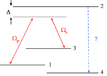
Figure 1: (Color online) Level scheme and coupling scheme. Level $4$ is very far from the other three.

We model the irreversible population decay from the intermediate state $\left|2\right\rangle$ by introducing an additional state $\left|4\right\rangle$, to which state $\left|2\right\rangle$ decays (see figure 1). In the absence of such a decay the Hamiltonian describing the enlarged four-state system reads (with $\hbar=1$):

$$H_{0}(t)=\left[\begin{array}[]{cccc}\omega_{1}&\Omega_{p}(t)e^{i(\omega_{21}-\Delta)t}&0&0\\ \Omega_{p}(t)e^{-i(\omega_{21}-\Delta)t}&\omega_{2}&\Omega_{s}(t)e^{-i(\omega_{23}-\Delta)t}&0\\ 0&\Omega_{s}(t)e^{i(\omega_{23}-\Delta)t}&\omega_{3}&0\\ 0&0&0&\omega_{4}\\ \end{array}\right]\,,$$ (1)

with $\omega_{4}<0$ well separated from the other levels, and $\omega_{mn}=\omega_{m}-\omega_{n}$. The population decay of state $\left|2\right\rangle$ to state $\left|4\right\rangle$ is modeled by a system-bath coupling Hamiltonian involving these two states, which in the non-rotating frame is given by:

$$H_{\text{dec}}=\left(\left|2\right\rangle\left\langle 4\right|+\left|4\right\rangle\left\langle 2\right|\right)\otimes\sum_{k}g_{k}\left(a_{k}+a_{k}^{\dagger}\right)\,.$$ (2)

In the rotating frame, the transformation to which is given by $T(t)=e^{i\omega_{1}t}\left|1\right\rangle\left\langle 1\right|+e^{i(\omega_{2}-\Delta)t}\left|2\right\rangle\left\langle 2\right|+e^{i\omega_{3}t}\left|3\right\rangle\left\langle 3\right|$, the Hamiltonian of the system becomes

$$H_{s}(t)=\left[\begin{array}[]{cccc}0&\Omega_{p}(t)&0&0\\ \Omega_{p}(t)&\Delta&\Omega_{s}(t)&0\\ 0&\Omega_{s}(t)&0&0\\ 0&0&0&\omega_{4}\\ \end{array}\right]\,,$$ (3)

and $H_{\text{dec}}$ changes accordingly:

$$H_{\text{dec}} = \left[e^{i(\omega_{2}-\Delta)t}\left|2\right\rangle\left\langle 4\right|+e^{-i(\omega_{2}-\Delta)t}\left|4\right\rangle\left\langle 2\right|\right]$$ (4)

$$\otimes \sum_{k}g_{k}\left(a_{k}+a_{k}^{\dagger}\right)\,.$$

The instantaneous eigenstates of the Hamiltonian $H_{s}(t)$ are ref:Vitanov1997 :

$$\left|+\right\rangle =\sin\varphi\sin\theta\left|1\right\rangle+\cos\varphi\left|2\right\rangle+\sin\varphi\cos\theta\left|3\right\rangle\,,$$ (5a)

$$\left|0\right\rangle =\cos\theta\left|1\right\rangle-\sin\theta\left|3\right\rangle\,,$$ (5b)

$$\left|-\right\rangle =\cos\varphi\sin\theta\left|1\right\rangle-\sin\varphi\left|2\right\rangle+\cos\varphi\cos\theta\left|3\right\rangle\,,$$ (5c)

where

$$\tan\theta(t) =\frac{\Omega_{p}(t)}{\Omega_{s}(t)}\,,$$ (6a)

$$\tan{2\varphi(t)} =\frac{2\Omega_{0}(t)}{\Delta(t)}\,,$$ (6b)

$$\Omega_{0}(t) =\sqrt{\Omega_{p}(t)^{2}+\Omega_{s}(t)^{2}}\,,$$ (6c)

and state $\left|4\right\rangle$ which is left unchanged by the transformation. The corresponding eigenvalues are $\omega_{+}=\Omega_{0}\cot\varphi$, $0$, $\omega_{-}=-\Omega_{0}\tan\varphi$ and $\omega_{4}$.

In the ideal case (in the absence of $H_{\text{dec}}$), perfect population transfer from $\left|1\right\rangle$ to $\left|3\right\rangle$ takes place. In particular, two different pulse sequences are possible, the intuitive and the counterintuitive sequences. In the intuitive sequence, the pump pulse $\Omega_{p}(t)$ precedes the Stokes pulse $\Omega_{s}(t)$; then for nonzero single-photon detuning $\Delta$ it can be shown that in the adiabatic limit the population remains at all times in state $\left|-\right\rangle$, which at $t=-\infty$ is equal to state $\left|1\right\rangle$ and at $t=\infty$ it is equal to state $\left|3\right\rangle$. Therefore, in the adiabatic limit there is a perfect population transfer from $\left|1\right\rangle$ to $\left|3\right\rangle$ ref:Vitanov97 analytic ; this process has recently been termed b-STIRAP (because it proceeds via the bright state $\left|-\right\rangle$) ref:b-STIRAP . For the counterintuitive pulse sequence, the pump pulse follows the Stokes pulse. Then the population is transferred through the dark state $\left|0\right\rangle$, which again is equal to $\left|1\right\rangle$ at $t=-\infty$ and to $\left|3\right\rangle$ at $t=\infty$.

In the non-ideal case of decaying state $\left|2\right\rangle$, the predictions change. In ref. ref:Vitanov1997 it has been shown that the instability of the intermediate state reduces the efficiency of the scheme. In particular it turns out that the intuitive sequence is more fragile than the counterintuitive one. Since these results have been obtained by means of a phenomenological Hamiltonian approach, it is natural to ask whether these results may change when a microscopic master equation approach is used. In the following we give the master equation describing the dissipative dynamics of the system.

According to the general theory by Davies ref:Davies1978 , recently applied to some time-dependent systems ref:Florio2006 , under the assumption of bath correlation times much smaller than the time of variation of the Hamiltonian, the master equation describes jumps between the instantaneous eigenstates of the time-dependent Hamiltonian. Since the Hamiltonian (4) involves only states $\left|2\right\rangle$ and $\left|4\right\rangle$, and since state $\left|2\right\rangle$ is not involved in the dark state $\left|0\right\rangle$, the only jumps allowed are $\left|+\right\rangle\leftrightarrows\left|4\right\rangle$ and $\left|-\right\rangle\leftrightarrows\left|4\right\rangle$. Therefore the master equation of our system is given by

$$\frac{\mathrm{d}\rho}{\mathrm{d}t} = -i[H_{s}(t),\rho]$$ (7)

$$+ \gamma_{+}(t)\left(\left|4\right\rangle\left\langle+\right|\rho\left|+\right\rangle\left\langle 4\right|-\tfrac{1}{2}\left\{\left|+\right\rangle\left\langle+\right|,\rho\right\}\right)$$

$$+ \gamma_{-}(t)\left(\left|4\right\rangle\left\langle-\right|\rho\left|-\right\rangle\left\langle 4\right|-\tfrac{1}{2}\left\{\left|-\right\rangle\left\langle-\right|,\rho\right\}\right)$$

$$+ \gamma_{+}^{exc}(t)\left(\left|+\right\rangle\left\langle 4\right|\rho\left|4\right\rangle\left\langle+\right|-\tfrac{1}{2}\left\{\left|4\right\rangle\left\langle 4\right|,\rho\right\}\right)$$

$$+ \gamma_{-}^{exc}(t)\left(\left|-\right\rangle\left\langle 4\right|\rho\left|4\right\rangle\left\langle-\right|-\tfrac{1}{2}\left\{\left|4\right\rangle\left\langle 4\right|,\rho\right\}\right)\,.$$

Here

$$\gamma_{+}(t) =\cos^{2}\varphi(t)|g(\tilde{\omega}_{+})|^{2}D(\tilde{\omega}_{+})(N(\tilde{\omega}_{+})+1)\,,$$ (8a)

$$\gamma_{-}(t) =\sin^{2}\varphi(t)|g(\tilde{\omega}_{-})|^{2}D(\tilde{\omega}_{-})(N(\tilde{\omega}_{-})+1)\,,$$ (8b)

are the decay rates of the states $\left|+\right\rangle$ and $\left|-\right\rangle$ toward state $\left|4\right\rangle$, corresponding to the Bohr frequencies $\tilde{\omega}_{\pm}=\omega_{\pm}+\omega_{2}-\omega_{4}$. The quantities $D(\tilde{\omega}_{\pm})$ and $N(\tilde{\omega}_{\pm})$ are respectively the densities of modes and the average numbers of photons in the reservoir at the relevant frequencies. The parameter $g(\tilde{\omega}_{\pm})$ gives the continuum-limit system-reservoir coupling strengths. We note that the factors $\cos^{2}\varphi$ and $\sin^{2}\varphi$ in Eq. (8) come from the calculation of the square moduli of the matrix elements of the system operator $\left|2\right\rangle\left\langle 4\right|+\left|4\right\rangle\left\langle 2\right|$ appearing in $H_{\text{dec}}$ between states $\left|4\right\rangle$ and $\left|+\right\rangle$, and between $\left|4\right\rangle$ and $\left|-\right\rangle$, respectively. Finally, the excitation rates are given by $\gamma_{\pm}^{exc}(t)=\gamma_{\pm}(t)N(\tilde{\omega}_{\pm})/(N(\tilde{\omega}_{\pm})+1)$ and vanish at zero temperature. This will be the case in the following sections.

III Rate Equations and Effective Hamiltonian

Introducing the density matrix decomposition in terms of the instantaneous eigenstates of the Hamiltonian $H_{s}(t)$,

$$\rho(t)=\sum_{ij}\rho_{ij}(t)\left|i(t)\right\rangle\left\langle j(t)\right|,$$ (9)

and substituting it into the master equation (7), one obtains a set of rate equations,

$$\dot{\rho}_{ij}(t)=\sum_{k}A_{ijkl}(t)\rho_{kl}(t)\,.$$ (10)

On the other hand, introducing the matrix of the density operator matrix elements in the time-dependent basis, i.e.

$$\bar{\rho}=\left[\rho_{ij}(t)\right]\,,$$ (11)

with $i,j=\pm,0$, one can prove (see appendix A) that the same rate equations can be obtained with a pseudo-Liouville equation, restricted to the subspace $\left|+\right\rangle$, $\left|0\right\rangle$, $\left|-\right\rangle$:

$$\dot{\bar{\rho}}=-i\left(H_{\text{eff}}\bar{\rho}-\bar{\rho}H_{\text{eff}}^{\dagger}\right)\,,$$ (12)

with

$$H_{\text{eff}}=\left[\begin{array}[]{cccc}\Omega_{0}\cot\varphi-i\Gamma\cos^{2}\varphi&i\dot{\theta}\sin\varphi&i\dot{\varphi}\\ -i\dot{\theta}\sin\varphi&0&-i\dot{\theta}\cos\varphi\\ -i\dot{\varphi}&i\dot{\theta}\cos\varphi&-\Omega_{0}\tan\varphi-i\Gamma\sin^{2}\varphi\\ \end{array}\right]\,,$$ (13)

where, reminding that $N(\tilde{\omega}_{\pm})=0$ at zero temperature and assuming flat reservoir spectrum ref:Petru , we have set $\Gamma=|g(\tilde{\omega}_{+})|^{2}D(\tilde{\omega}_{+})=|g(\tilde{\omega}_{-})|^{2}D(\tilde{\omega}_{-})$.

The comparison of this Hamiltonian with the phenomenological Hamiltonian of Eq. (4) of ref:Vitanov1997 , i.e.:

$$\dot{\bar{\rho}}=-i\left(H_{\text{phen}}\bar{\rho}-\bar{\rho}H_{\text{phen}}^{\dagger}\right)\,,$$ (14)

where

$$H_{\text{phen}}=\left[\begin{array}[]{cccc}\Omega_{0}\cot\varphi-i\Gamma\cos^{2}\varphi&i\dot{\theta}\sin\varphi&i\dot{\varphi}+\frac{i}{2}\Gamma\sin 2\varphi\\ -i\dot{\theta}\sin\varphi&0&-i\dot{\theta}\cos\varphi\\ -i\dot{\varphi}+\frac{i}{2}\Gamma\sin 2\varphi&i\dot{\theta}\cos\varphi&-\Omega_{0}\tan\varphi-i\Gamma\sin^{2}\varphi\\ \end{array}\right]\,,$$ (15)

shows that the only difference is in terms (1,3) and (3,1). The two Hamiltonians (13) and (15) are written down in the basis $\left|+\right\rangle$, $\left|0\right\rangle$, $\left|-\right\rangle$ (not $\left|1\right\rangle$, $\left|2\right\rangle$, $\left|3\right\rangle$).

More details of the derivation of the effective Hamiltonian are given in Appendix A.

IV Comparison of the two approaches

We shall now compare the two models, the one using the effective Hamiltonian (13) derived from the master equation, and the phenomenological one using the Hamiltonian (15). We shall consider, as in ref:Vitanov1997 , two pulses of the form

$$\Omega_{1}(t)=\frac{\alpha}{T\sqrt{2}}\,\mathrm{sech}\left(\frac{t}{T}\right)\cos\left[\frac{\pi}{4}\left(\tanh\frac{t}{T}+1\right)\right]\,,$$ (16a)

$$\Omega_{2}(t)=\frac{\alpha}{T\sqrt{2}}\,\mathrm{sech}\left(\frac{t}{T}\right)\sin\left[\frac{\pi}{4}\left(\tanh\frac{t}{T}+1\right)\right]\,,$$ (16b)

where $T$ determines the widths of the pulses while $\alpha$ their intensities, so that $\alpha T$ gives a measure of each pulse area.

IV.1 Weak damping ($\Gamma T\ll 1$)

Intuitive pulse sequence – For the intuitive sequence (i.e., when $\Omega_{p}=\Omega_{1}$ and $\Omega_{s}=\Omega_{2}$), the effective and phenomenological models deliver essentially the same results. This feature derives from the fact that the adiabatically transferred population is that of state $\left|-\right\rangle$. In the weak-damping limit, the dominant source of decay is the population decay of $\left|-\right\rangle$ itself due to the term (3,3) in both the Hamiltonians $H_{\text{eff}}$ and $H_{\text{phen}}$, thereby diminishing the effects of the off-diagonal terms and in particular of $\frac{i}{2}\Gamma\sin 2\varphi$ in (1,3) and (3,1), which are the only difference between the two models. Hence the decay of the final state, with a good approximation, is given by

$$P_{3}\simeq\exp\left[-2\Gamma\int_{-\infty}^{\infty}\sin^{2}\varphi(t)\text{d}t\right].$$ (17)

Figure 2 shows the asymptotic value of $P_{3}$ as a function of $\Gamma$ for both models, and shows the nearly perfect agreement of the two predictions, in particular the exponential dependence on $\Gamma$.

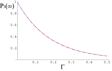
Figure 2: (Color online) Asymptotic values of population $P_{3}$ for the phenomenological and effective (perfectly superimposed) model for the intuitive sequence, as functions of $\Gamma$ (in units of $T^{-1}$), for $\alpha T=10$, $\Delta T=1$.

Counterintuitive pulse sequence – For the counterintuitive sequence ($\Omega_{s}=\Omega_{1}$ and $\Omega_{p}=\Omega_{2}$), still under the weak damping conditions, we can study the evolution through the adiabatic elimination, assuming that the states $\left|+\right\rangle$ and $\left|-\right\rangle$ are not very much populated during the process. We decompose the state vector in the adiabatic basis as $\left|\psi\right\rangle=a_{+}\left|+\right\rangle+a_{0}\left|0\right\rangle+a_{-}\left|-\right\rangle$, and the Schrödinger equation becomes a set of linear differential equations for the probability amplitudes,

$$i\frac{\text{d}}{\text{d}t}\left[\begin{array}[]{c}a_{+}\\ a_{0}\\ a_{-}\end{array}\right]=H\,\left[\begin{array}[]{c}a_{+}\\ a_{0}\\ a_{-}\end{array}\right],$$ (18)

with $H=H_{\text{eff}}$ or $H=H_{\text{phen}}$, depending on the model considered. By setting $\dot{a}_{+}\approx\dot{a}_{-}\approx 0$, we find $a_{+}$ and $a_{-}$ as functions of $a_{0}$, and substitute these expressions in the equation for $\dot{a}_{0}$, which assumes the form

$$\dot{a}_{0}(t)=-A(t)a_{0}(t)\,,$$ (19)

where $A(t)$ has one of the following expressions depending on the model one is considering:

$$A^{\text{phen}}(t)=\frac{\dot{\theta}^{2}(\Gamma+2i\Omega_{0}\cot 2\varphi)}{(i\Omega_{0}\cot\varphi+\Gamma\cos^{2}\varphi)(-i\Omega_{0}\tan\varphi+\Gamma\sin^{2}\varphi)+\dot{\varphi}^{2}-\frac{1}{4}\Gamma^{2}\sin^{2}2\varphi}$$ (20)

for the phenomenological model, and

$$A^{\text{eff}}(t)=\frac{\dot{\theta}^{2}[\Gamma(\cos^{4}\varphi+\sin^{4}\varphi)+2i\Omega_{0}\cot 2\varphi]}{(i\Omega_{0}\cot\varphi+\Gamma\cos^{2}\varphi)(-i\Omega_{0}\tan\varphi+\Gamma\sin^{2}\varphi)+\dot{\varphi}^{2}}$$ (21)

for the effective model.

Equation (19) has the very simple solution

$$a_{0}(t)=a_{0}(-\infty)\exp\left[-\int_{-\infty}^{t}A(t^{\prime})\mathrm{d}t^{\prime}\right]\,,$$ (22)

which corresponds to the dark-state population

$$P_{0}(t)=\exp\left[-2\int_{-\infty}^{t}\Re(A(t^{\prime}))\mathrm{d}t^{\prime}\right]\,.$$ (23)

For the phenomenological model, according to ref:Vitanov1997 , at the first order in the parameter $\Gamma$, we find

$$P_{3}^{\text{phen}}(\infty)=\exp\left[-2\Gamma\int_{-\infty}^{\infty}\frac{\dot{\theta}^{2}}{\Omega_{0}^{2}+\dot{\varphi}^{2}}\,\mathrm{d}t^{\prime}\right]\,,$$ (24)

while for the effective model the result is

$$P_{3}^{\text{eff}}(\infty)=\exp\bigg{[}-2\Gamma\int_{-\infty}^{\infty}\frac{\dot{\theta}^{2}\left(\sin^{4}\varphi+\cos^{4}\varphi\right)}{\Omega_{0}^{2}+\dot{\varphi}^{2}}\mathrm{d}t^{\prime}\bigg{]},$$ (25)

where we have taken into account the fact that for the counterintuitive sequence, we have $P_{0}(-\infty)=P_{1}(-\infty)=1$ and $P_{0}(\infty)=P_{3}(\infty)$.

Since $\sin^{4}\varphi+\cos^{4}\varphi\leq 1$, it is evident that $P_{3}^{\text{eff}}(\infty)>P_{3}^{\text{phen}}(\infty)$. Numerical results agree with this prediction, as shown in Fig.  3.

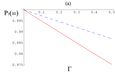
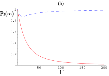
Figure 3: (Color online) Post-pulse values of population $P_{3}$ for the phenomenological (solid red line) and effective (dashed blue line) model for the counterintuitive pulse sequence, as functions of $\Gamma$ (in units of $T^{-1}$) for weak damping only (a) and in a wide range (b). Relevant parameters: $\alpha T=10$, $\Delta T=1$.

It can be shown that as $\alpha$ increases the agreement between the results obtained in the adiabatic approximation and the numerical results improves. Indeed, generally speaking, higher $\alpha$ means higher Rabi frequencies between the states, which put the system more under adiabatic conditions ref:Vitanov1997b . It is also worth nothing that the higher $\alpha$ the closer to unity are the values of $P_{3}$ for $\Gamma=0$. Again, this depends on the validity of the adiabatic approximation, according to which the levels $\left|+\right\rangle$ and $\left|-\right\rangle$ are not populated, so that the population transfer by $\left|0\right\rangle$ is more and more efficient, without losses of population to the other two levels.

IV.2 Strong damping: numerical simulations

Figure 3b shows the complete dependence of $P_{3}^{\text{eff}}(\infty)$ and $P_{3}^{\text{phen}}(\infty)$ on $\Gamma$ and, in particular, the strong damping limit. While $P_{3}^{\text{phen}}(\infty)$ decays as $\Gamma$ increases, it is well visible that $P_{3}^{\text{eff}}(\infty)$ reaches higher values and in particular approaches $1$ for high values of $\Gamma$. Such a behavior can be explained in terms of generalized quantum Zeno effect ref:QZE1 ; ref:QZE2 , meaning that the strong decay produces a separation of the Hilbert space into Zeno subspaces. If $\Gamma$ is much larger than other quantities ($\Omega_{0}$, $\dot{\varphi}$, $\dot{\theta}$), we can split the Hamiltonian $H_{\text{eff}}$ as a sum of the unperturbed one, which contains only terms proportional to $\Gamma$, and a perturbation, that is

$$H_{\text{eff}}= \ +\left[\begin{array}[]{cccc}-i\Gamma\cos^{2}\varphi&0&0\\ 0&0&0\\ 0&0&-i\Gamma\sin^{2}\varphi\\ \end{array}\right]$$ (29)

$$+\left[\begin{array}[]{cccc}\Omega_{0}\cot\varphi&i\dot{\theta}\sin\varphi&i\dot{\varphi}\\ -i\dot{\theta}\sin\varphi&0&-i\dot{\theta}\cos\varphi\\ -i\dot{\varphi}&i\dot{\theta}\cos\varphi&-\Omega_{0}\tan\varphi\\ \end{array}\right]\,.$$ (33)

The three eigenvalues of the unperturbed (first) part of the Hamiltonian are $\lambda=-i\Gamma\cos^{2}\varphi,-i\Gamma\sin^{2}\varphi$ and 0, corresponding to the eigenstates $\left|+\right\rangle$, $\left|-\right\rangle$, $\left|0\right\rangle$. Since $\Gamma$ is very high, for $\varphi\not=\pi/4$ the three eigenstates correspond to very different eigenvalues and the presence of the perturbation only slightly changes the eigenvalues and eigenstates of the total Hamiltonian, so that the three states turn out to be essentially uncoupled throughout the process. On the contrary, when $\varphi=0$ the states $\left|0\right\rangle$ and $\left|-\right\rangle$ could be coupled by the terms $\mp i\dot{\theta}\cos\varphi$. However, it is easy to see that when $\varphi=0$, $\theta(t)$ is a constant function and $\dot{\theta}=0$. Moreover, when $\varphi=\pi/4$ the states $\left|+\right\rangle$ and $\left|-\right\rangle$ are coupled by the terms $\pm i\dot{\varphi}$, but the relevant transitions are unimportant since the only state with nonzero population is $\left|0\right\rangle$. Therefore, there are no transitions between the adiabatic states, and $\left|0\right\rangle$ can transfer the population from level $\left|1\right\rangle$ to level $\left|3\right\rangle$ without decay since the corresponding eigenvalue is essentially zero.

In the phenomenological model, we have

$$H_{\text{phen}}= \ \left[\begin{array}[]{cccc}-i\Gamma\cos^{2}\varphi&0&\frac{i}{2}\Gamma\sin 2\varphi\\ 0&0&0\\ \frac{i}{2}\Gamma\sin 2\varphi&0&-i\Gamma\sin^{2}\varphi\\ \end{array}\right]$$ (37)

$$+\left[\begin{array}[]{cccc}\Omega_{0}\cot\varphi&i\dot{\theta}\sin\varphi&i\dot{\varphi}\\ -i\dot{\theta}\sin\varphi&0&-i\dot{\theta}\cos\varphi\\ -i\dot{\varphi}&i\dot{\theta}\cos\varphi&-\Omega_{0}\tan\varphi\\ \end{array}\right]\,,$$ (41)

and the eigenvalues of the unperturbed (first) part of the Hamiltonian are $\lambda=0,0$ and $-i\Gamma$, corresponding to the eigenstates $\left|0_{1}\right\rangle=\left|0\right\rangle$, $\left|0_{2}\right\rangle=\sin\varphi\left|+\right\rangle+\cos\varphi\left|-\right\rangle$ and $\left|-i\Gamma\right\rangle=\cos\varphi\left|+\right\rangle-\sin\varphi\left|-\right\rangle$, respectively. Since $\Gamma$ is very large, the perturbation does not couple the state $\left|-i\Gamma\right\rangle$ to the doublet (the other two states in the degenerate subspace), but the states of the doublet can be coupled by the perturbation. In fact, the restriction of the perturbation to the doublet is

$$H_{\text{doublet}}=\left[\begin{array}[]{cc}0&-i\dot{\theta}\\ i\dot{\theta}&0\end{array}\right]\,,$$ (42)

and since $\theta$ in the counterintuitive sequence varies from $0$ to $\pi/2$, there is complete population inversion in the doublet. Therefore, since $\left|0_{1}\right\rangle(-\infty)=\left|0\right\rangle(-\infty)=\left|1\right\rangle$, the final state of the system is $\left|0_{2}\right\rangle(\infty)=\left|-\right\rangle(\infty)=\left|1\right\rangle$, and there is no population transfer to level $\left|3\right\rangle$. Summarizing, in the strong coupling for a counterintuitive pulse sequence, the effective model predicts a complete population transfer whereas the phenomenological model predicts essentially no transfer.

Let us now turn to the intuitive pulse sequence. We have already seen that for small values of $\Gamma$ the population transfer from $\left|1\right\rangle$ to $\left|3\right\rangle$ is very low. This feature, which is common to the two models, relies on very different physical mechanisms. Let us start considering that in the intuitive sequence, for the phenomenological model, at $t=-\infty$ we have $\left|1\right\rangle=\left|-\right\rangle=\left|0_{2}\right\rangle$, which, according to the previous analysis, undergoes a complete transition toward state $\left|0_{1}\right\rangle$, so that the final state is $\left|0_{1}\right\rangle(\infty)=\left|0\right\rangle(\infty)=\left|1\right\rangle$, and there is no transfer to state $\left|3\right\rangle$. Figure 4a shows this behavior. In the effective model, the system starts from $\left|-\right\rangle(-\infty)=\left|1\right\rangle$ and there are transitions between states $\left|+\right\rangle$ and $\left|-\right\rangle$ around $\varphi=\pi/4$; the entire subspace spanned by these two states decays. Therefore, a complete loss of probability of the system characterizes the dynamics in this case. Figure 4b illustrates this feature.

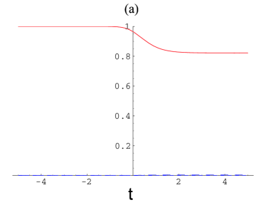
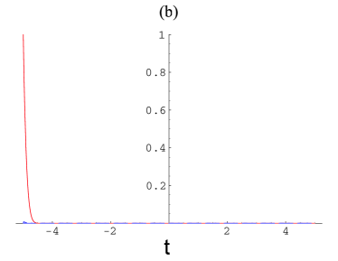
Figure 4: (Color online) Evolution of the populations in the strong damping limit, according to the effective model in the intuitive sequence (a) and in the phenomenological model in the counterintuitive sequence (b): $P_{1}$ as a solid (red) line, $P_{2}$ as a dotted (green) line and $P_{3}$ as a dashed (blue) line. Populations $P_{2}$ and $P_{3}$ are essentially zero everywhere. Time is measured in units of $T$. Relevant parameters are $\alpha T=10$, $\Gamma T=500$, $\Delta T=1$.

V Conclusions

In this paper we have shown that the phenomenological and effective models for a laser-driven three-state $\Lambda$-system under dissipative dynamics give different descriptions.

We have shown that the two relevant non-Hermitian Hamiltonian models differ, in the adiabatic basis, in off-diagonal terms which couple levels 1 and 3 and which are proportional to the decay constant $\Gamma$. This suggests that the discrepancy between predictions coming from the two models may increase as the decay rate increases. Both analytical and numerical results confirm this insight. Indeed, for weak damping the predictions from both models are essentially the same, while in the strong damping limit the difference is evident. Specifically, in the strong damping limit, for the counterintuitive pulse sequence, there is a significant difference in the values of the post-pulse population of the target state: according to the phenomenological model there should be no transfer from state $1$ to state $3$, while the effective model predicts almost complete population transfer as $\Gamma$ increases. We note that, even though for the intuitive pulse sequence the predictions for the post-pulse population of level $3$ are the same for both models, the physical mechanisms that lead to this result are very different for large $\Gamma$. In fact, in the phenomenological model the population is kept in state $1$, while in the effective model there is no final population in state $3$ because all the states have undergone a total decay.

The most important result in this paper is the prediction of a complete population transfer for the counterintuitive sequence in the strong damping limit; this result is of potential interest in applications of STIRAP schemes in the manipulation of quantum states.

Appendix A Derivation of the Effective Model

In this appendix we derive the effective Hamiltonian model in (13) from the master equation (7).

Substituting (9) into (7), and assuming zero temperature ($\tilde{\gamma}$’s $=0$) one obtains the following set of rate equations in the adiabatic basis:

$$\dot{\rho}_{00}=-\dot{\theta}\sin\varphi\,\rho_{+0}-\dot{\theta}\sin\varphi\,\rho_{0+}-\dot{\theta}\cos\varphi\,\rho_{-0}-\dot{\theta}\cos\varphi\,\rho_{0-}\,,$$ (43a)

$$\dot{\rho}_{++}=-\gamma_{+}\,\rho_{++}+\dot{\varphi}\,\rho_{-+}+\dot{\varphi}\,\rho_{+-}+\dot{\theta}\sin\varphi\,\rho_{0+}+\dot{\theta}\sin\varphi\,\rho_{+0}\,,$$ (43b)

$$\dot{\rho}_{--}=-\gamma_{-}\,\rho_{--}-\dot{\varphi}\,\rho_{-+}-\dot{\varphi}\,\rho_{+-}+\dot{\theta}\cos\varphi\,\rho_{0+}+\dot{\theta}\cos\varphi\,\rho_{+0}\,,$$ (43c)

$$\dot{\rho}_{+0}=\left(-i\omega_{+0}-\frac{\gamma_{+}}{2}\right)\rho_{+0}+\dot{\theta}\sin\varphi\,\rho_{00}+\dot{\varphi}\rho_{-0}-\dot{\theta}\sin\varphi\,\rho_{++}-\dot{\theta}\cos\varphi\,\rho_{+-}\,,$$ (43d)

$$\dot{\rho}_{+-}=\left(-i\omega_{+-}-\frac{\gamma_{+}+\gamma_{-}}{2}\right)\rho_{+-}+\dot{\theta}\sin\varphi\,\rho_{0-}+\dot{\varphi}\rho_{--}+\dot{\theta}\cos\varphi\,\rho_{+0}-\dot{\varphi},\rho_{++}\,,$$ (43e)

$$\dot{\rho}_{0-}=\left(-i\omega_{0-}-\frac{\gamma_{-}}{2}\right)\rho_{0-}-\dot{\theta}\sin\varphi\,\rho_{+-}-\dot{\theta}\cos\phi\,\rho_{--}-\dot{\varphi}\,\rho_{0+}+\dot{\theta}\cos\varphi\,\rho_{00}-\dot{\varphi}\,\rho_{++}\,,$$ (43f)

and the Hermitian conjugates of the last three equations. Equations involving level $4$ are not shown, since they don’t play any role in the effective model. As a consequence the effective model does not conserve the total probability. It is straightforward to see that substituting the Hamiltonian model in (13) into (12), one obtains exactly the same rate equations. Therefore we conclude that $H_{\text{eff}}$ represents the effective Hamiltonian of the system.

Appendix B Strong damping in the bare basis

In this appendix we show how to treat the strong damping dynamics in the bare basis $\{\left|1\right\rangle,\left|2\right\rangle,\left|3\right\rangle\}$. In ref. ref:Vitanov1997 the starting point of the treatment is to give the phenomenological Hamiltonian:

$$H_{phen}^{bare}=\left[\begin{array}[]{ccc}0&\Omega_{p}(t)&0\\ &&\\ \Omega_{p}(t)&\Delta-i\Gamma&\Omega_{s}(t)\\ &&\\ 0&\Omega_{s}(t)&0\\ \end{array}\right]\,,$$ (44)

which, transformed to the adiabatic basis $\{\left|+\right\rangle,\left|0\right\rangle,\left|-\right\rangle\}$, gives Eq. (15). Equation (44) clearly indicates that in the strong damping limit state $\left|2\right\rangle$ is well separated from the other states, so that the coupling scheme does not allow to transfer population from state $\left|1\right\rangle$ to state $\left|3\right\rangle$.

In the master equation approach, the effective Hamiltonian in the bare basis assumes a much more complicated form which does not allow to separate the three bare states. Indeed, since the effective Hamiltonian is related to the phenomenological one by the relation

$$H_{\text{eff}}=H_{\text{phen}}-i\frac{\Gamma}{2}\sin 2\varphi\left[\begin{array}[]{ccc}0&0&1\\ 0&0&0\\ 1&0&0\\ \end{array}\right]\,,$$ (45)

we find that the inverse transformation from the adiabatic to the bare basis gives:

$$H_{\text{eff}}^{\text{bare}}=H_{\text{phen}}^{\text{bare}}-i\frac{\Gamma}{2}\sin 2\varphi\left[\begin{array}[]{ccc}2\sin\varphi\cos\varphi\sin^{2}\theta&\cos 2\varphi\sin\theta&2\sin\varphi\cos\varphi\sin\theta\cos\theta\\ \cos 2\varphi\sin\theta&-\sin 2\varphi&\cos 2\varphi\cos\theta\\ 2\sin\varphi\cos\varphi\sin\theta\cos\theta&\cos 2\varphi\cos\theta&2\sin\varphi\cos\varphi\cos^{2}\theta\\ \end{array}\right],$$ (46)

which clearly shows the impossibility of separating state $\left|2\right\rangle$ from the other ones. Therefore the only basis in which the strong-damping dynamics can be easily explained is the adiabatic one.

References

(1) U. Gaubatz, P. Rudecki, S. Schiemann, K. Bergmann, J. Chem. Phys. 92, 5363
(1990).
(2) S. Schiemann, A. Kuhn, S. Steuerwald, K. Bergmann, Phys. Rev. Lett. 71, 3637 (1993).
(3) N. V. Vitanov, M. Fleischhauer, B. W. Shore and K. Bergmann, Adv. At. Mol. Opt. Phys. 46, 55 (2001).
(4) N. V. Vitanov, T. Halfmann, B. W. Shore and K. Bergmann, Ann. Rev. Phys. Chem. 52, 763 (2001).
(5) K. Bergmann, H. Theuer, and B. W. Shore, Rev. Mod. Phys. 70, 1003 (1998).
(6) P. Král, I. Thanopoulos, and M. Shapiro, Rev. Mod. Phys. 79, 53 (2007).
(7) N. V. Vitanov and S. Stenholm, Opt. Commun. 135, 394 (1997).
(8) P. A. Ivanov, N. V. Vitanov, and K. Bergmann, Phys. Rev. A 70, 063409 (2004).
(9) P. A. Ivanov, N. V. Vitanov, and K. Bergmann, Phys. Rev. A 72, 053412 (2005).
(10) N. V. Vitanov and S. Stenholm, Phys. Rev. A 56, 1463 (1997).
(11) C. W. Gardiner and P. Zoller, Quantum Noise (Springer-Verlag, Berlin, 2000).
(12) H.-P. Breuer and F. Petruccione, The Theory of Open Quantum Systems (Oxford University Press, Oxford, 2002).
(13) E. B. Davies and H. Spohn, J. Stat. Phys. 19, 511 (1978).
(14) G. Florio, P. Facchi, R. Fazio, V. Giovannetti, and S.Pascazio, Phys. Rev. A 73, 022327
(2006).
(15) A. Carollo, M. França Santos and V. Vedral, Phys. Rev. Lett. 96, 020403 (2006).
(16) M.S. Sarandy and D.A. Lidar, Phys. Rev. Lett. 95, 250503 (2005).
(17) M. Scala, B. Militello, A. Messina, J. Piilo and S. Maniscalco, Phys. Rev. A 75, 013811
(2007).
(18) M. Scala, B. Militello, A. Messina, S. Maniscalco, J. Piilo and
K.-A Suominen, Phys. Rev. A 77, 043827 (2008).
(19) M. Wilczewski and M. Czachor, Phys. Rev. A 80, 013802
(2009).
(20) M. Wilczewski and M. Czachor, Phys. Rev. A 79, 033836 (2009).
(21) M. Scala, R. Migliore and Messina, J. Phys. A: Math. Theor. 41, 435304 (2008).
(22) N. V. Vitanov and S. Stenholm, Phys. Rev. A 55, 648 (1997).
(23)
J. Klein, F. Beil, and T. Halfmann, Phys. Rev. A 78, 033416 (2008).
(24) B. Militello, A. Messina and A. Napoli, Fortschr. Phys. 49, 1041 (2001).
(25)P. Facchi and S. Pascazio, Phys. Rev. Lett. 89, 080401 (2002).