Quasi-two dimensional dipolar scattering

Abstract

We study two body dipolar scattering with one dimension of confinement. We include the effects of confinement by expanding this degree of freedom in harmonic oscillator states. We then study the properties of the resulting multi-channel system. We study the adiabatic curves as a function of $D/l$, the ratio of the dipolar and confinement length scales. There is no dipolar barrier for this system when $D/l<0.34$. We also study the WKB tunneling probability as a function of $D/l$ and scattering energy. This can be used to estimate the character of the scattering.

I introduction

There has been great progress in the production of ultracold polar molecules gspm ; carr and ultracold dipolar collisions have now been experimentally observed ni . The dipolar interaction is: $V_{dd}=d^{2}{1-3(\hat{z}\cdot\vec{r})^{2}\over r^{3}}$, where $d$ is the induced dipole moment along the field axis ($z$). When this is included in the ultracold environment the scattering properties are intriguing universal ; roudnev ; NJP . For example, dipolar collisions are not Wigner suppressed at threshold; rather non-zero partial wave cross sections go to a constant as energy goes to zero threshold . These ultracold molecular systems present exciting avenues to study chemical reactions at ultracold temperatures with unprecedented control hudson ; chem ; chemkrems . There is a down side to chemical reactions, it may shorten trapping lifetimes and prevent the production of degenerate dipolar gases. To further control the collisions one could use confinement and produce lower dimensional quantum gases. By placing the ultracold molecules in a 1D optical lattice aligned with the polarization axis, one would remove the possibility of the molecules approaching each other along the attractive configuration of the interaction. In the strong trapping limit, this would make the interaction a purely repulsive $d^{2}/\rho^{3}$ potential. This would inhibit the particles from reaching the short range where they would chemically react. Beyond few body physics, ultracold 2D systems have been used to study the BKT phase transition BKT and quasi-condensation 2dnist . Adding dipoles to these systems could lead to exotic dipolar many body systems buchler and quantum memories rabl .

The production of 2D dipolar gases would be a valuable addition to the study of ultracold gases. They will offer further control over collisions and enable production of exotic many body systems. In an effort to bolster their production, we study basic properties of the 2D dipolar system. We are most interested in understanding when there is a dipolar barrier and how resilient a barrier it is. Previous studies of ultracold 2D scattering have focused on ultracold atoms petrov and inelastic collisions li . These theories were based on the assumption that the short range interaction is much smaller than the confinement length. We will use the same assumption here, but we allow the dipolar length scale to be both large or small compared to the confinement length scale. Confined dipolar systems have been considered in 1D dipolar sing , but to the knowledge of the author, no one has yet studied quasi 2D dipolar scattering. Here we study the scattering of two point dipoles under 1 dimension of confinement. By considering channels formed by the eigenstates of the confinement Hamiltonian which are coupled to each other by the dipolar interaction, we are able to study a standard multi-channel scattering problem. With this model we address an important issue: when can the particles be prevented from reaching short range. This work shows when confinement can be used to effectively shield the molecules from short range chemical reaction processes chem . In addition, we offer an estimate of character of the scattering, i.e. threshold or semi-classical. This will be important to understand the interactions and the properties of the resulting many body system. Furthermore, we address whether or not this system behaves similarly to a pure 2D system. This comparison allows one to predict the 2 body scattering properties of the system easily. The rest of the paper contains a review of the scattering equations, then a study of the adiabatic curves, and finally a study of the WKB tunneling probability. This allows rough scattering characteristics to be determined about the 2D dipolar system.

II Equations of motion

The Schrödinger Equation for two dipoles with 1 dimension of confinement is

$$\left(-{\nabla^{2}\over 2}+{z^{2}\over 2l^{4}}+D{1-3(\hat{z}\cdot\hat{r})^{2}\over r^{3}}\right)\psi={\mu E}\psi.$$ (1)

Here we assume the particles are polarized along the confinement axis ($z$). The length scales of this system are the dipolar length $D=\mu d^{2}/\hbar^{2}$ and the confinement length $l=\sqrt{\hbar/\mu\omega}$ where $\mu$ is the reduced mass and $\omega$ is the frequency. The corresponding energy scales are $E_{D}=\hbar^{2}/2\mu D^{2}$ and $\hbar\omega$. Additionally, there is the scattering energy $E$, and this has a length scale of $k^{-1}$ where $k^{2}=2\mu E/\hbar^{2}$. The parameters of interest in this system will be the ratio of the length scales $\bar{D}=D/l$ and the scattering energy. By varying $\bar{D}$, one will achieve the collisional control.

To study this system, we expand the wavefunction in harmonic oscillator states in the confinement direction, $\chi_{n}(z)$, and partial waves in the azimuthal coordinate, $e^{im\varphi}$. Using these expansions the total wavefunction is: $\psi=\sum_{mn}e^{im\varphi}\chi_{n}(z){\phi_{mn}(\rho)\over\sqrt{\rho}}$ gu , and this allows us to integrate out $z$. Now using $D$ to rescale Eq. (1), we obtain a multi-channel radial Schrödinger equation describing quasi 2D dipolar scattering:

$$\left(-{1\over 2}{d^{2}\over d\tilde{\rho}^{2}}+{m^{2}-1/4\over 2\tilde{\rho}^{2}}+\bar{D}^{2}n-{E\over E_{D}}\right)\phi_{mn}(\tilde{\rho})=$$

$$-\sum_{mn^{\prime}}U_{nn^{\prime}}(\tilde{\rho})\phi_{mn^{\prime}}(\tilde{\rho})$$ (2)

where $\tilde{\rho}=\rho/D$ and

$$\langle\chi_{n}|V_{dd}|\chi_{n^{\prime}}\rangle=d^{2}U_{nn^{\prime}}(\rho)$$

$$U_{nn^{\prime}}(\rho)=\int dz\chi^{*}_{n}(z){1-3(\hat{z}\cdot\vec{r})^{2}\over(z^{2}+\rho^{2})^{3/2}}\chi_{n^{\prime}}(z).$$

We set the lowest threshold to zero and consider only even or odd $n$ because parity is conserved by the interaction. The short range length scale is assumed to be much smaller than both $l$ and $D$. This length scale is where the interaction deviates from the dipolar interaction, and is typically of order 100$a_{0}$ ($\sim$5nm). This length scale will most likely be the depolarization length where the molecules reorient relative to each other. Once the particles reach this length scale more complex interaction dynamics occur, such as chemical reactions and are far beyond the scope of this work.

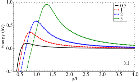
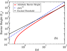
Figure 1: (Color Online) (a) The adiabatic potential energy curves, $V_{0}(\rho/l)$, are shown for $\bar{D}=0.5$ (solid black), $\bar{D}=1$ (red circles), $\bar{D}=2$ (blue x), and $\bar{D}=5$ (green square) in harmonic oscillator units. (b) The height of the dipolar barrier as a function of $\bar{D}$. The first excited threshold, $2\bar{D}^{2}$ (solid black) and $\bar{D}^{5/2}$ (blue dashed) are plotted in dipolar energy units.

To study the character of the system, we first look at the adiabatic curves. These are obtained by diagonalizing the potentials in Eq. (2) as a function of $\rho$. We also include the standard diagonal correction from the kinetic energy which is ${-\hbar^{2}\over 2\mu}\langle 0|d^{2}/d\rho^{2}|0\rangle$ where $|0\rangle$ is the lowest adiabatic eigenstate and depends on $\rho$. First we will look at the adiabatic potentials in confinement units. In Fig. 1 (a) the lowest $m=0$ adiabatic potential energy curves are shown for $\bar{D}=0.5$ (solid black), $\bar{D}=1$ (red circles), $\bar{D}=2$ (blue x), and $\bar{D}=5$ (green square). This figure shows that as $\bar{D}$ is increased the barrier becomes higher and moves out in $\rho/l$. In Fig. 1 (b) we have shown the height of the adiabatic barrier as a function of $\bar{D}$ (solid red) in dipolar units, which more readily translate to scattering physics. We have also plotted the energy of the first excited threshold, $2\bar{D}^{2}$ (solid black) and $\bar{D}^{5/2}$ (blue dashed) buchler . In this figure the barrier height goes to zero at non-zero $\bar{D}$. This will be explored below.

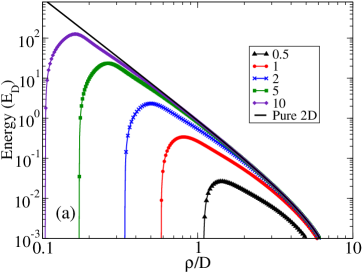
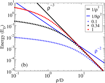
Figure 2: (Color Online) (a) The lowest adiabatic curve on a log-log scale for various values of $\bar{D}$, which are: 0.5 (black triangle), 1 (red circles), 2 (blue x), 5 (green square), and 10 (violet diamond). Compared with the pure 2D scattering potential (solid black). (b) The lowest diabatic curve is shown for $\bar{D}$=0.1 (blue +), 0.34 (black triangle), and 1 (red circles) as a function of $\tilde{\rho}$. Also shown is pure dipolar repulsion (solid black) and the absolute value of the attractive 2D centrifugal term (solid blue).

To relate these adiabatic potentials to the scattering character it is convenient to look at them in dipolar units; in these units the long range interaction has a simple form: $(m^{2}-1/4)/2\tilde{\rho}^{2}+1/\tilde{\rho}^{3}$. The scattering on this potential is understood and has a universal form ticknor2d . Thus it will be important to see when the adiabatic curves deviate from the pure 2D potential and this will offer an idea of when the scattering deviates from the pure 2D case.

The adiabatic potentials in the dipole units are shown in Fig. 2 (a) for $\bar{D}$ equal to: 0.5 (black triangle), 1 (red circles), 2 (blue x), 5 (green square), and 10 (violet diamond), and the pure 2D case is solid black. For large values of $\bar{D}$, there is a large dipolar barrier. The kinetic energy correction makes a significant contribution for large $\bar{D}$. Importantly the dipolar barrier closely mimics the pure 2D case. As $\bar{D}$ is decreased, the region where the potential deviates from the repulsive $1/\tilde{\rho}^{3}$ moves out in $\tilde{\rho}$. This deviation from the pure 2D case is very clear at $\bar{D}=0.5$ (black). If $\bar{D}$ is further decreased, eventually there is no barrier below $0.34$ $(\equiv\bar{D}_{c})$.

In Fig. 2 (b), we illustrate why there is no barrier below $\bar{D}_{c}$, and it is essentially a signal channel phenomena. We plot the diabatic curves, $U_{00}(\tilde{\rho})$, for different values of $\bar{D}$=0.1 (blue +), 0.25 (green dashed), 0.5 (black triangle), and 1 (red circles) as a function of $\tilde{\rho}$. The pure 2D repulsion ($1/\tilde{\rho}^{3}$) is shown as a solid black line and the absolute value of the attractive centrifugal term is show as solid blue ($1/8\tilde{\rho}^{2}$). At small values of $\rho/l$, the ground state mode samples a large portion of the dipolar interaction. This softens the interaction, making it less repulsive than the centrifugal term at small $\rho$. When $\bar{D}$ is decreased, the softened interaction is pushed to larger $\tilde{\rho}$. If $\bar{D}$ is small enough the dipolar interaction entirely looses the competition with the attractive centrifugal term and there is no barrier. For collisions in the first excited state ($n=1$ and $m=0$), $\bar{D}_{c}^{1}=0.95$. This is important for identical for fermions, which will be able to collide in this channel without Wigner suppression.

III tunneling probability

We now investigate the tunneling behavior and some scattering properties of the quasi 2D system. To do this we assume that the scattering energy is smaller than the confinement energy and this means there is only one open channel (a unique combination of $n$ and $m$). We solve Eq. (2) with the Johnson Log-derivative johnson and match to energy normalized Bessel functions. The cross section is $\sigma={4\over k}\sin^{2}(\delta)$ where $\delta$ is the scattering phase shift. For pure threshold dipolar scattering the system behaves as a system with a 2D scattering length verhaar of $a_{s}/D=e^{2\gamma+ln(2)}\sim 6.344$, where $\gamma$ is Euler constant Arnecke . The $m$=0 cross section diverges as energy goes to zero. Furthermore, in contrast to 3D the non-zero partial waves are Wigner suppressed and go to zero as energy goes to zero threshold ; ticknor2d .

 

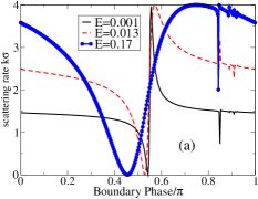
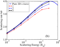
Figure 3: (Color Online) (a) The scattering rate, $4\sin^{2}(\delta)$, as a function of the inner boundary phase for $\bar{D}$=1 at different energies: 0.001 (solid red), 0.013 (black dashed), and 0.17 (blue with circles). (b) The background scattering rate as a function of the scattering energy for $\bar{D}$ equal to 1 (red circles), 2 (open blue squares), and 5 (black triangle). The pure 2D scattering is shown as a solid blue curve.

To explore the long range scattering of this system as a function of $\bar{D}$ and the scattering energy, we use the inner boundary condition to study the influence of the short range on the scattering. In future studies we envision a full 3D solution combined with a frame transformation frame to capture the short range dynamics of the scattering. This would resemble the formalism used in quantum defect theory QDT . For this study, we simply place an inner wall behind the adiabatic barrier where the short range dynamics occur. A good example of the information provided by varying inner boundary condition is shown in Fig. 3 (a). In this figure $\bar{D}=1$ and the energies are: 0.001 (solid black), 0.013 (red dashed), and 0.17 (blue circles). The central feature is the shape resonance we want to analyze, and the other two resonances are narrow multi-channel Feshbach resonances. We use up to $n=8$ to converge these scattering calculations.

The scattering phase shift can be written as $\delta\approx\delta_{bg}+\tan^{-1}\left[\Gamma\cot(\phi_{SR}-\pi/2)\right]$ where $\delta_{bg}$ is the back ground phase shift, $\Gamma$ is resonance width, and $\phi_{SR}$ is the phase acquired inside the barrier. $\delta_{bg}$ is the scattering phase shift acquired by the long range scattering and $\phi_{SR}$ is the impact of the short range dynamics on the scattering. Here we directly alter $\phi_{SR}$ with the inner boundary condition. This leads to a direct method to estimate the width of the resonance produced by the dipolar barrier in a scattering process for a given $\bar{D}$ and energy. From curves like those in Fig. 3 (a) we are able to extract both $\delta_{bg}$ and $\Gamma$ as a function of $\phi_{SR}$. We first look at the background scattering rate, which is shown in Fig. 3 (b) as a function of the scattering energy for $\bar{D}$ equal to 1 (red circles), 2 (open blue squares), and 5 (black triangle). The important feature of this figure is that as $\bar{D}$ is increased, the cross section becomes more like the pure 2D case (solid blue). Additionally as energy is lowered, the systems becomes more like the pure 2D case. Restating the important point, for small $\bar{D}$ the scattering rate is smaller than the pure 2D scattering rate. This allows it to be used as an upper estimate of the scattering proprieties.

We will now study the WKB tunnelling probability, and use this quantity to estimate of how likely the system is to access short range. Additionally the WKB tunnelling probability can be used to estimate $\Gamma$ berry . Resonances in this system will be connected to the threshold resonances which occur in dipolar scattering as the polarization is increased You ; CTPR ; roudnev . The confinement will modify the resonant character of the system, especially when there is a barrier to the scattering process. As $\bar{D}$ is increased, the system gains another bound state and there will be a resonance. We can estimate $\Gamma$ when the system is tunneling dominated. The WKB tunneling estimate will not be accurate when the system is scattering near the top of the barrier where much more complex scattering dynamic occur.

The WKB tunnelling probability is:

$$P_{T}=e^{-2\gamma},\gamma=\int_{cf}d\rho\kappa(\rho)$$ (3)

where $\kappa=\sqrt{2\mu(V_{0}^{L}(\rho)-E)}$, where $V_{0}^{L}$ is the lowest adiabatic potential including the Langer correction $(m^{2}-{1\over 4}\rightarrow m^{2})$. The integral is over the classically forbidden ($cf$) region for a given energy. In Fig. 4 (a) $P_{T}$ is shown as a function energy for $\bar{D}$ equal to 1 (black line), 2 (red circles), 3 (blue triangles), 4 (maroon squares), and 5 (violet diamond). We also show the fitted widths from the scattering calculations for $\bar{D}$ =1 (black solid circles), 2 (red open circles), and 3 (large blue triangle) as a function of energy. The important feature of this data is that the energy dependence of the resonance width is correct; as the energy is decreased the width also decreases. One short coming of this analysis is that the tunneling width depends on the short range scattering. We try to avoid this impact by placing the hard wall near where the adiabatic potentials predict the barrier to end. However we only include the widths for $\bar{D}$ = 1, 2, and 3 because for larger $\bar{D}$ the widths are very sensitive to the location of the inner boundary as channel couplings become very large. The resonances become more narrow the further back the wall is placed and requires many more channels to be converged.

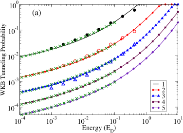
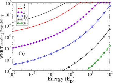
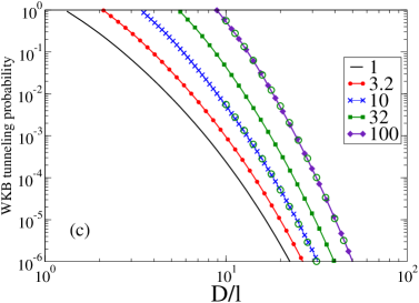
Figure 4: (Color Online) (a) The WKB tunneling probability is shown as a function of energy for $\bar{D}$ equal to 1 (black line), 2 (red circles), 3 (blue triangles), 4 (maroon squares), and 5 (violet diamond). The fitted resonance widths from the scattering calculations are shown for $\bar{D}$= 1 (black circles), 2 (red open circles), 3 (blue open triangle). The green x’s in each plot are the fitted $P_{T}$ from Eq. (4). (b) The WKB tunneling probability is shown as a function of energy for $\bar{D}$ equal to 1 (black line), 2 (red circles), 5 (violet diamond), 10 (open blue circles), 20 (open black triangle), and 30 (open green squares). (c) $P_{T}$ is shown as a function of $\bar{D}$ for the energies: 1 (black), 3.2 (red with circles), 10 (blue x), 32 (green square), and 100 (violet diamond). The open green circles are the fit: $139.3({E\over E_{D}})^{2}e^{-5.86\bar{D}^{2/5}}$ for $E/E_{D}$=10 and 100 and show very good agreement.

Here we provide an estimate of the WKB probability with a fit to the numerical data:

$$\ln(P_{T})=a\bar{D}^{2/5}+b\bar{D}^{-1/10}$$ (4)

$$a=-5.17436+0.143167y+0.0093433y^{2}$$

$$b=5.16437+1.61799y+0.135513y^{2}$$

where $y=\log(E/E_{D})$. This fit is accurate to better than 15$\%$ for $\bar{D}$ between 1 to 10 and energies between $10^{-6}$ to $10^{-1}$. This was to capture the tunneling probability in the threshold regime and is much better for low energy. Ref. buchler obtained an energy independent tunneling probability proportional to $e^{-5.86\bar{D}^{2/5}}$, the numerical $P_{T}$ strongly deviates from this form as $\bar{D}$ becomes small and when the scattering energy is near the top of the barrier. This fit will be useful when estimating the nature of the scattering.

In the semi-classical regime, $E/E_{D}>1$, there are many partial waves scattering and the scattering rate approaches $4\sqrt{\pi Dk}$ ticknor2d . The s-wave contribution is only a fraction of the scattering events. For non-zero $m$, the system has a repulsive centrifugal barrier in addition to the dipolar repulsion; this will greatly suppress the tunnelling to short range. However to calculate the WKB tunneling probability, the short range interaction must be taken into account and for this reason it will be omitted here.

As $\bar{D}$ is increased the impact of the s-wave reaching short range becomes much smaller. To illustrate the suppression of the tunnelling rates for $m=0$, we have plotted $P_{T}$ as a function of both energy and $\bar{D}$ in Fig. 4 (c). The WKB tunneling probability is shown as a function of energy for $\bar{D}$ equal to 1 (black line), 2 (red circles), 5 (violet diamond), 10 (open blue circles), 20 (open black triangle), and 30 (open green squares). This figure demonstrates that as $\bar{D}$ is increased the tunneling rate will dramatically drop. The functional form of $P_{T}$ is nearly $c_{E}e^{-5.86\bar{D}^{2/5}}$. For $\bar{D}$ between 10 and 100 and energy between 10 and 100, we find:

$$P_{T}=139.3(E/E_{D})^{2}e^{-5.86\bar{D}^{2/5}}$$ (5)

This reproduces $P_{T}$ to within about 30$\%$ over the stated parameter range. The fit is best when the energy is not near the top of the barrier. In Fig. 4 (c) this fit is shown as green circles for both $E/E_{D}$ =10 and 100. Between the regimes when the energy is near the top of the barrier, the tunneling behavior is complex and will in fact involve much more than just tunneling dynamics to understand. For this reason, we omit the parameter region from the fit. We have used up to $n$=8 and this is enough to converge $P_{T}$ for the parameter range shown.

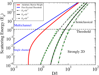
Figure 5: (Color Online)The character of the quasi 2D scattering as a function of $E/E_{D}$ vs. $\bar{D}$. The excited threshold (solid blue) and the height of adiabatic barrier (solid red) are shown. The WKB tunneling probability contour for $P_{T}=$ $10^{-2}$ (dashed black), $10^{-3}$ (solid black), and $10^{-4}$ (dash dot black) are plotted. The green x’s in each plot are the fitted $P_{T}$ from Eq. (4) and the greens circles are the fit for the semi-classical energy regime from Eq. (5).

Fig. 5 shows an estimate of effectiveness of the barrier and the character of quasi 2D scattering as a function of $E/E_{D}$ vs. $\bar{D}$. The curves in this figure are: the first excited threshold (solid blue), the height of adiabatic barrier (red curve), the WKB tunneling probability contour for $P_{T}=10^{-2}$ (dashed black), $10^{-3}$ (solid black), and $10^{-4}$ (dash dot black). Additionally in Fig. 5 the green x’s and open circles are the contours from the fits, they agree well with the full data. The important feature of this figure is that it offers a quick estimate of whether or not a quasi 2D dipolar system will effectively produce a barrier to the short range. Once the parameters are below the dipolar barrier (red line), the system must tunnel to reach the short range interaction. When the parameters of the system are among or below the black contours the dipolar barrier will suppress the systems ability to reach short range where inelastic collisions occur. More contours indicating higher levels of suppression were omitted because they offered little additional information. In this case of highly suppressed tunneling systems, their behavior will be like the pure 2D dipolar scattering, especially at threshold ticknor2d . If the systems is near or above the dipolar barrier or if there is no dipolar barrier ($\bar{D}<\bar{D}_{c}$), the scattering dynamics will be rich and require the short range interaction to be included. For parameters above the solid blue line there will be many open confinement thresholds and the scattering dynamics will be very complex with many possible inelastic processes between confinement thresholds.

In Fig. 5 the thin horizontal dashed line at $E/E_{D}=1$ denotes the transition between threshold and semi-classical scattering behavior. Above this line, many non-zero partial waves will contribute to the scattering and the cross section will behave as $k\sigma\propto\sqrt{Dk}$ (total scattering rate). When the scattering is in this regime, the s-wave scattering will be a fraction of total scattering events, and the larger number of non-zero partial wave scattering events might further suppress the inelastic losses. To know this for sure, one would have to include the short range interaction.

IV Conclusions

In this paper we have studied quasi 2 dimensional dipolar scattering. We included the effects of confinement by expanding this degree of freedom in harmonic oscillator states, and studied the properties of the resulting multi-channel system. We examined the adiabatic curves as a function of $\bar{D}$, and found there is a dipolar barrier only when $\bar{D}>\bar{D}_{c}=0.34$. We used the lowest adiabatic curve to obtain the WKB tunneling probability of this system. We found fits of $P_{T}$ in the threshold and semi-classical scattering regime. When the system is tunneling dominated these will be good estimates of how likely particles are to make it to the short range. This might also be related to the width of resonances in the system. Fig. 5 offers a quick means to estimate whether an effective barrier will be produced by a molecular system in an optical lattice.

The physical implications of this work are simple, try to maximize $\bar{D}={\mu^{3/2}d^{2}\omega^{1/2}\over\hbar^{5/2}}$. $\bar{D}$ must exceed 0.34 for there to be a dipolar barrier, and should be much larger to significantly inhibit the particles from reaching the short range. If one desires to have a gas in the threshold regime, one must also keep $E/E_{D}={\mu^{3}d^{4}E\over\hbar^{6}}$ less than 1. This will leads to an optimal value of $d$, which is set by the external electric field. To give a physical example, set $E\sim 100$nK and $\omega\sim 50$kHz. Then for LiCs, $\bar{D}$ can exceed 100. However the cost of this would be to make $E_{D}$ minuscule, less than 1nK, and this would lead to semi-classical scattering. To maintain the thresholds scattering one would have set the field to $d_{b}{\cal E}/B\sim 0.2$ where $B$ is the rotational constant of ${}^{1}\Sigma$ molecule and $d_{b}$ is the bare dipole moment. At this field $\bar{D}\sim 2.7$ and $E/E_{D}\sim 0.2$, which is in the threshold regime and produces $P_{T}\sim 2\cdot 10^{-2}$. An important physical example is RbK gspm ; ni , for this system if the field is $d_{b}{\cal E}/B\sim 5$, the field will produce $\bar{D}\sim 2$, $E/E_{D}\sim 0.1$ and $P_{T}\sim 3\cdot 10^{-2}$. To further decrease $P_{T}$ lowering the scattering energy might be more feasible than producing a tighter trap. This system will have threshold dipolar scattering and will help suppress the chemical reactions chem . There are several important future directions of this research. For example how does the scattering behave when $E/\hbar\omega>2$ and there are many open confinement thresholds? How are the resonances in this quasi 2D systems related to the threshold resonances in 3D dipolar systems? To address this question a short range interaction must be included. This will also open up many avenues for further and more complete studies of these collisions.

^∗Current Address: Theoretical Division, Los Alamos National Laboratory, Los Alamos, New Mexico 87545, USA

References

- (1) K.-K. Ni, et al., Science 322 231, (2008).
- (2) For a recent review see: L. D. Carr et al. New J. Phys. 11, 055049 (2009).
- (3) K.-K. Ni et al., arXiv:1001.2809.
- (4) C. Ticknor, Phys. Rev. Lett., 100 133202 (2008); Phys. Rev. A 76, 052703 (2007).
- (5) V. Roudnev and M. Cavagnero, Phys. Rev. A, 79 014701 (2009); J. Phys. B, 42, 044017 (2009).
- (6) J. L. Bohn, M. Cavagnero, and C. Ticknor, New J. Phys. 11 055039 (2009).
- (7) H. R. Sadeghpour, et al., J. Phys. B 33, R93 (2000).
- (8) E. R. Hudson, et al., Phys. Rev. A 73, 063404 (2006).
- (9) S. Ospelkaus, et al., arXiv:0912.3854.
- (10) R. V. Krems, Physical Chemistry Chemical Physics 10, 4079 (2008).
- (11) Z. Hadzibabic, et al., Nature (London) 441, 1118 (2006)
- (12) P. Clade, C. Ryu, A. Ramanathan, K. Helmerson, and W. D. Phillips, Phys. Rev. Lett. 102, 170401 (2009).
- (13) H. P. Büchler, et al., Phys. Rev. Lett. 98, 060404 (2007).
- (14) P. Rabl and P. Zoller, Phys. Rev. A 76, 042308 (2007).
- (15) D. S. Petrov and G. V. Shlyapnikov, Phys. Rev. A, 64, 012706 (2001); D. S. Petrov, M. Holzmann, and G. V. Shlyapnikov, Phys. Rev. Lett. 84, 2551 (2000).
- (16) Z. Li et al., Phys. Rev. Lett., 100, 073202 (2008); Z. Li and R. V. Krems, Phys. Rev. A 79, 050701(R) (2009).
- (17) S. Sinha and L. Santos, Phys. Rev. Lett. 99, 140406 (2007).
- (18) Z.-Y. Gu and S. W. Quian, Phys. Lett. A 136, 6 (1989).
- (19) C. Ticknor, Phys. Rev. A. 80 052702 (2009).
- (20) B. R. Johnson, J. Comput. Phys. 13, 445 (1973).
- (21) B. J. Verhaar, et al., J. Phys. A: Math. Gen. 17, 595 (1984).
- (22) F. Arnecke, H. Friedrich, and P. Rabb, Phys. Rev. A, 78, 052711 (2008).
- (23) C. H. Greene, Phys. Rev. A 36 4236 (1987); B. E. Granger and D. Blume Phys. Rev. Lett. 92 133202 (2004).
- (24) M. Aymar, C. H. Greene, and E. Luc-Koenig Rev. Mod. Phys. 68 1015 (1996); B. Gao, Phys. Rev. A 78, 012702 (2008).
- (25) M. V. Berry, Proc. Phys. Soc., 88, 285 (1966).
- (26) M. Marinescu and L. You, Phys. Rev. Lett. 81, 4596 (1998).
- (27) C. Ticknor and J. L. Bohn Phys. Rev. A 72, 032717 (2005).