K-Shell Photoabsorption Studies of the Carbon Isonuclear Sequence

Abstract

K-shell photoabsorption cross sections for the isonuclear C I - C IV ions have been computed using the R-matrix method. Above the K-shell threshold, the present results are in good agreement with the independent-particle results of Reilman & Manson (1979). Below threshold, we also compute the strong $1s\rightarrow np$ absorption resonances with the inclusion of important spectator Auger broadening effects. For the lowest $1s\rightarrow 2p,3p$ resonances, comparisons to available C II, C III, and C IV experimental results show good agreement in general for the resonance strengths and positions, but unexplained discrepancies exist. Our results also provide detailed information on the C I K-shell photoabsorption cross section including the strong resonance features, since very limited laboratory experimental data exist. The resultant R-matrix cross sections are then used to model the Chandra X-ray absorption spectrum of the blazar Mkn 421.

1 Introduction

The inner-shell excitation and ionization features of cosmically abundant elements fall in the spectral ranges covered by the high-resolution X-ray spectrometers onboard the Chandra and XMM-Newton observatories. The detailed structure and wavelengths of absorption resonances of a given element depend on its ionization and chemical state. High resolution X-ray spectroscopy of these features can in principle be used to probe the physics and chemistry of astrophysical plasmas. Inner-shell photoabsorption resonances have proven particularly useful for investigating the chemical composition of the interstellar gas in the line-of-sight toward bright sources of X-ray continuum radiation, as demonstrated in the pioneering study of Schattenburg & Canizares (1986) (see also Paerels et al., 2001; Takei et al., 2002; de Vries et al., 2003; Juett et al., 2004, 2006; Ueda et al., 2005; Yao & Wang, 2006; Yao et al., 2009; Kaastra et al., 2009).  Ness et al. (2007) were able to identify several ionization stages of oxygen in the post-outburst circumstellar material of the recurrent nova RS Oph based on the prominent $1s\rightarrow 2p$ resonance.

These studies have all employed oxygen and higher $Z$ elements. Carbon is the fourth most abundant element in the Galaxy (after H, He, and O), but has not yet been exploited as an X-ray photoabsorption diagnostic. It presents a special challenge for X-ray transmission spectroscopy. X-ray instruments often employ visible/UV light blocking filters based on carbon compounds that are robust to space deployment. These filters imprint strong C K-edge absorption signatures on X-ray spectra, rendering difficult the disentanglement of weaker astrophysical absorption features. The task is hampered further still by a current lack of data describing the expected absorption edge structure and resonances for neutral and ionized C.

In order to investigate C absorption features, we perform detailed R-matrix calculations of the K-shell photoabsorption cross-sections of C I - C IV. These cross sections are then used to interpret the x-ray spectra from a high-quality Chandra observation of the blazar Mkn 421 and determine relative carbon-ion abundances.

2 Theoretical Methodology

The specific processes of interest are the K-shell photoexcitation of the carbon-ion ground state,

$$h\nu+1s^{2}2l^{q} \rightarrow 1s2l^{q}np\ ,$$ (1)

followed by two competing decay routes. First, there is participator Auger decay

$$1s2l^{q}np \rightarrow 1s^{2}2l^{q-1}+e^{-}\ ,$$ (2)

where the valence electron $np$ takes part in the autoionization process; the decay width therefore scales as $1/n^{3}$ and goes to zero near the K-shell threshold. There is also the more important spectator Auger decay

$$1s2l^{q}np \rightarrow 1s^{2}2l^{q-2}np+e^{-}\ ,$$ (3)

where the valence electron $np$ does not take part in the autoionization process, giving instead a decay width that is independent of $n$. Spectator Auger decay is therefore the dominant decay route as $n\rightarrow\infty$ and gives a smooth cross section as the K-shell threshold is approached; above each threshold, K-shell photoionization to the $1s2l^{q}$ states occurs instead. We note that for $n=2$, there is no distinction between spectator and participator channels.

To account for photoionization to the participator channels, we use the standard R-matrix method (Burke & Berrington, 1993; Berrington et al., 1995) and expand the total wavefunction in a basis consisting of free electron orbitals $\epsilon l^{\prime}$ coupled to each of the ground-state and singly-excited $1s^{2}2l^{q-1}$ target wavefunctions, plus bound orbitals $np$ coupled to the K-shell vacancy target wavefunctions $1s2l^{q}$. However, the infinite number of $1s^{2}2l^{q-2}np+e^{-}$ spectator decay channels are impossible to include implicitly in such an R-matrix expansion; instead, they are accounted for via an optical potential approach (Gorczyca & Robicheaux, 1999). The target energy for each closed channel $1s2l^{q}np$ is modified within a multi-channel quantum defect theory approach as

$$E_{1s2l^{q}}\rightarrow E_{1s2l^{q}}-i\Gamma_{1s2l^{q}}/2\ ,$$ (4)

where $\Gamma_{1s2l^{q}}$ is the $1s2l^{q}\rightarrow 1s^{2}2l^{q-2}+e^{-}$ Auger width. This enhanced R-matrix method was shown to be successful in describing experimental synchrotron measurements for Ar I (Gorczyca & Robicheaux, 1999), O I (Gorczyca & McLaughlin, 2000), and Ne I (Gorczyca, 2000), and Chandra high-resolution spectroscopic observations for oxygen ions (Juett et al., 2004; Garcia et al., 2005) and neon ions (Juett et al., 2006). We compute the $1s2l^{q}$ Auger widths by applying the Smith time-delay method (Smith, 1960) to the photoabsorption R-matrix calculation of the neighboring $1s^{2}2l^{q-1}$ carbon ion. Since $1s\rightarrow 2p$ photoabsorption of the $1s^{2}2l^{q-1}$ ion gives an intermediate $1s2l^{q}$ resonance, the subsequent Auger decay to the $1s^{2}2l^{q-2}+e^{-}$ channel can be analyzed to obtain the Auger width.

It is also important to obtain accurate target wavefunctions using a single orthogonal orbital basis, and this is problematic since orbital relaxation occurs when the $1s^{2}2l^{q-1}$ states are excited to the $1s2l^{q}$ K-shell-vacancy states (the $2l$ electrons are now only screened by one, not two, $1s$ electrons). We account for orbital relaxation by using additional pseudoorbitals as follows. A basis of physical $1s$, $2s$, and $2p$ orbitals is first constructed by performing Hartree-Fock calculations for the $1s^{2}2l^{q-1}$ ground states. Then multiconfiguration Hartree-Fock (MCHF) calculations (Fischer et al., 1997) are performed for the $1s2l^{q}$ K-shell-excited states, including all configurations obtained from single and double promotions to the $n=3$ shell, to obtain $\overline{3s}$, $\overline{3p}$, and $\overline{3d}$ pseudoorbitals. All target states are then described by a configuration-interaction (CI) expansion using all configurations consistent with single and double promotions out of the $1s^{2}2l^{q-1}$ and $1s2l^{q}$ states, using the six $1s$, $2s$, $2p$, $\overline{3s}$, $\overline{3p}$, and $\overline{3d}$ orbitals. Our computed R-matrix C II - C V target energies are shown in Tables I-IV, respectively, and compared to the currently recommended NIST values for the $1s^{2}2l^{q-1}$ singly-excited states. To our knowledge, there are no experimental or theoretical values for the K-shell-excited $1s2l^{q}$ energies for comparison except for the $1s2s^{2}2p^{2}(^{4}P)$ state of C II. The energy of this state corresponds to the K-shell threshold in the photoabsorption of C I and was measured to be $296.07\pm 0.2$ eV by (Bruch et al., 1985), which is in good agreement with our predicted value of 296.096 eV.

Given target wavefunctions, we construct total wavefunctions by coupling an additional electron orbital. Standard R-matrix calculations were then performed including only the participator channels, and by investigating the behavior near the $1s2l^{q-1}$ resonances, the Auger widths of Eq. 4 are determined. These R-matrix Auger widths are listed in Tables V-VIII and compared to multiconfiguration Breit-Pauli (MCBP) and multiconfiguration Dirac-Fock (MCDF) results. Given the Auger widths, the spectator Auger channels are also included in the optical potential R-matrix calculations for C I - C IV to yield cross sections with the correct resonance widths for $n>2$.

3 Cross Section Results

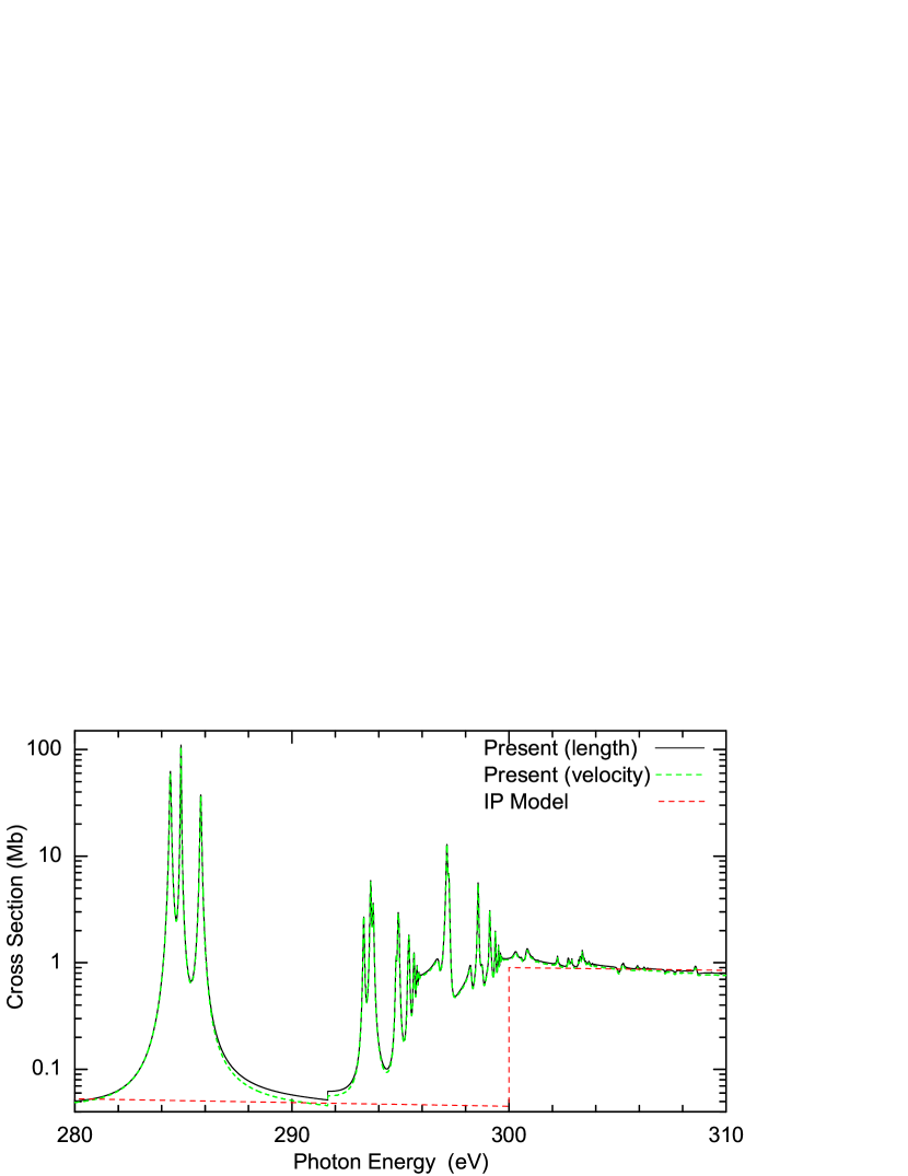
Figure 1: C I photoabsorption cross sections: R-matrix length and velocity results compared to the independent-particle results of Reilman & Manson (1979).

Our results for the C I photoabsorption cross section are shown in Fig. 1. To our knowledge, there is very limited experimental data for comparison purposes available in the literature (Jannitti et al., 1990; Nicolosi et al., 1991; Henke et al., 1993) and primarily from dual laser plasma experiments. From their Dual Laser Plasma (DLP) experiments Jannitti and co-workers (Jannitti et al., 1990; Nicolosi et al., 1991) were able to make preliminary identifications of the $1s\rightarrow 2p$ resonances in the vicinity of the K-edge. However, it should be stressed that experimental data on atomic carbon that does exists in the literature was obtained at very low resolution and performed using the Dual Laser Plasma (DLP) technique as pioneered by Carroll & Kennedy (1977). The dual plasma technique is useful for obtaining absorption spectra over a wide energy range (Jannitti et al., 1990; O’Sullivan et al., 1996). Their interpretation, however, can be extremely complicated due to ions being distributed over various charge states in both the ground and metastable-states, and the presence of a plasma can affect energy levels, as can post-collision interactions (PCI).

Theoretical cross-sections are available in the literature from the independent-particle (IP) model (Reilman & Manson, 1979; Yeh, 1993) that include the direct photoionization continuum (but not the $1s\rightarrow np$ resonance contributions) as does the scaled hydrogenic work of Verner et al. (1993); Verner & Yakovlev (1995). Ab initio work has also been carried out using the R-matrix approach (Petrini & da Silva, 1999; McLaughlin, 2001). Petrini & da Silva (1999) performed R-matrix calculations on this complex at energies above the hole states included in their work. No resonance structure was obtained in their work, since they were mainly interested in determining the shake up process (2s $\rightarrow$ 2p and 3s, and 2p $\rightarrow$ 3p excitations) in the photon energy range 25 to 45 Rydbergs, i.e. $\sim$ 340 eV to 612 eV, which is well above the carbon K-edge. They conclude that the 2s $\rightarrow$ 3s excitation dominates the shake up process and is about a factor of 2 smaller than in the case of boron (Badnell et al., 1997). In addition the 2s shake off process (at most 20%) would lead to the production of C III 1s^-1 hole states which can then Auger decay only to CIV 1s²2p. In contrast to this, the R-matrix work of McLaughlin (2001) catered for resonances in the vicinity of the carbon K-edge and showed strong resonance structure which was missing from various other theoretical approaches.

Our results for the C I photoabsorption cross section, using both length and velocity forms of the dipole operator, are shown in Fig. 1. For exact wavefunctions, the two results will be identical, and the excellent agreement between our two cross sections is an indication that we have obtained fairly accurate R-matrix wavefunctions. We find similar excellent agreement between length and velocity results for C II - C IV photoabsorption and therefore only show length results in the remainder of the paper. IP results are also shown in Fig. 1, which are seen to be in good agreement with our R-matrix cross section above the K-shell threshold.

Our computed $1s2s^{2}2p^{2}(^{4}P)$ K-shell threshold at 296.10 eV is in good agreement with the experimentally observed values of 296.2$\pm$0.5 eV by (Bisgaard et al., 1978) and 296.07$\pm$0.2 eV by (Bruch et al., 1985) and with the theoretical value of 296.02 eV from a UHF-SCF approximation. The discontinuity around 291.6 eV in the R-matrix results is due to the turn-off of Auger broadening below $n=3$ to prevent double counting of the Auger width of the $n=2$ resonance (the $1s2s^{2}2p^{2}$ resonances only decay to participator channels). This discontinuity of $1.1\times 10^{-2}$ Mb is very small compared to the large resonance features of $10^{1}-10^{2}$ Mb.

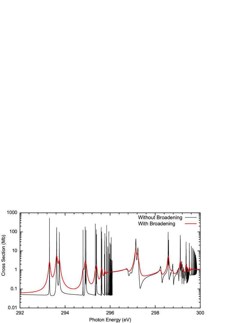
Figure 2: C I photoabsorption cross sections for $n\geq 3$ without (black) and with (red) spectator Auger broadening effects.

The importance of including spectator Auger decay channels via the optical potential approach can be seen in Fig. 2. Our results are shown with and without the spectator broadening effect. Whereas the spectator-broadened results show the physically-correct constant Auger width near threshold, the unbroadened results have widths that approach zero near threshold and are therefore impossible to resolve using a finite set of energy mesh points. Results are not shown for the lowest $1s2s^{2}2p^{2}$ resonances since these are not affected by spectator broadening.

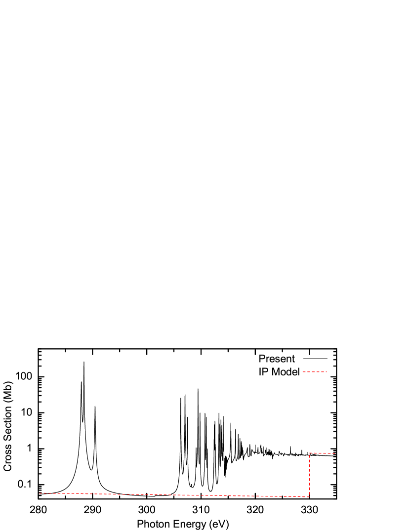
Figure 3: C II photoabsorption cross sections.

The K-shell cross section for C II is shown in Fig. 3 for the entire $1s\rightarrow np$ photoabsorption resonance region, and for the above-threshold $1s\rightarrow e^{-}$ photoionization region, where it is seen to be in fairly good agreement with the IP results of Reilman & Manson (1979). We note that the IP results are tabulated on a sparse grid, and for C I are provided at photon energies of 270 eV, 300 eV, and 330 eV, so that the results shown here are straight-line interpolations and do not exhibit the unsmooth energy dependence found in our R-matrix cross sections.

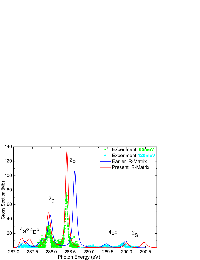
Figure 4: The $1s\to 2p$ photoabsorption for an admixture of $80\%$ ground-state $1s^{2}2s^{2}2p(^{2}P)$ and $20\%$ metastable state $1s^{2}2s2p^{2}(^{4}P)$ C II ions. Experimental measurements (Schlachter et al., 2002) are performed with two separate spectral resolutions of 65 meV and 120 meV. The theoretical cross sections are summed incoherently for an $80\%$ ground-state and $20\%$ metastable state admixture and then convoluted with a 65 meV or 120 meV FWHM Gaussian. Also shown are earlier R-matrix results (Schlachter et al., 2002)

For C II, there also exist experimental and earlier R-matrix results, but only for the $1s\rightarrow 2p$ resonances (Schlachter et al., 2002). In that experiment, in addition to the C II $1s^{2}2s^{2}2p(^{2}P)$ ground state, there was a $\approx 20$% $1s^{2}2s2p^{2}(^{4}P)$ metastable-state fraction, giving additional resonances not included in our calculations for Fig 3. Thus we performed an additional R-matrix photoabsorption calculation from the metastable state, including all quartet, rather than doublet, total symmetries, and then added the ground and metastable cross sections together with weightings of 80% and 20%, respectively. These results are shown in Fig. 4 along with the earlier results. For the two strongest ${}^{2}P$ and ${}^{2}D$ resonances, where the experimental resolution was 65 meV, we find good agreement with the experimental resonance positions, but both present and earlier R-matrix resonance strengths are found to be significantly greater than the measured strengths. The second set of experimental results was taken at 120 meV for the weaker resonances, and here we find that our resonance positions are in error by as much as 0.5 eV and our strengths are again greater than experiment.

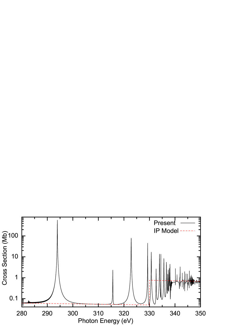
Figure 5: C III photoabsorption cross sections.

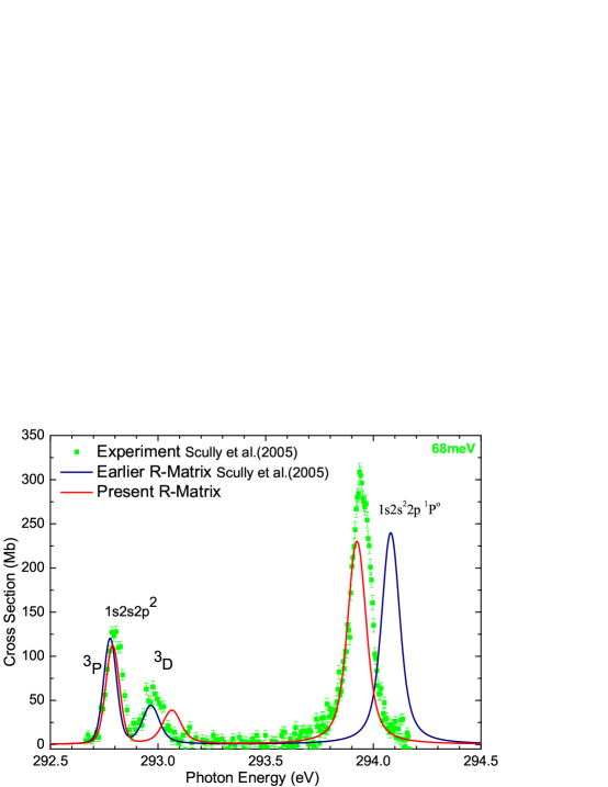
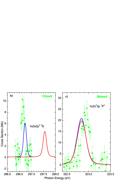
Figure 6: Present R-matrix cross section vs. experimental and earlier R-matrix results (Scully et al., 2005) for the $1s\to 2p,3p$ resonancs of C III. The theoretical curves are determined by considering an admixture of $68\%$ of the ground state and $32\%$ of the metastable state and are convoluted with a FWHM Gaussian given by the experimental resolution. In a), the $1s2s2p^{2}\,(^{3}P,\,^{3}D)$ and $1s2s^{2}2p^{2}\,(^{1}P)$ resonances are shown at a spectral resolution of 68 meV, b) shows the $1s2s2p^{2}\,(^{3}S)$ resonance at a resolution of 133 meV, and c) shows the $1s2s^{2}3p\,(^{1}P)$ resonance at a spectral resolution of 200 meV.

The C III photoabsorption cross section for the entire K-edge region is shown in Fig. 5 and compared to the IP results above threshold, where good agreement is again obtained. Results for the lowest $1s\rightarrow 2p,3p$ resonances are shown in Fig. 6. For the dominant $1s2s^{2}2p(^{1}P)$ resonance, both R-matrix photoabsorption strengths are now less than the experimental value (Scully et al., 2005), but there is good agreement for the second-strongest $1s2s2p^{2}(^{3}P)$ resonance.

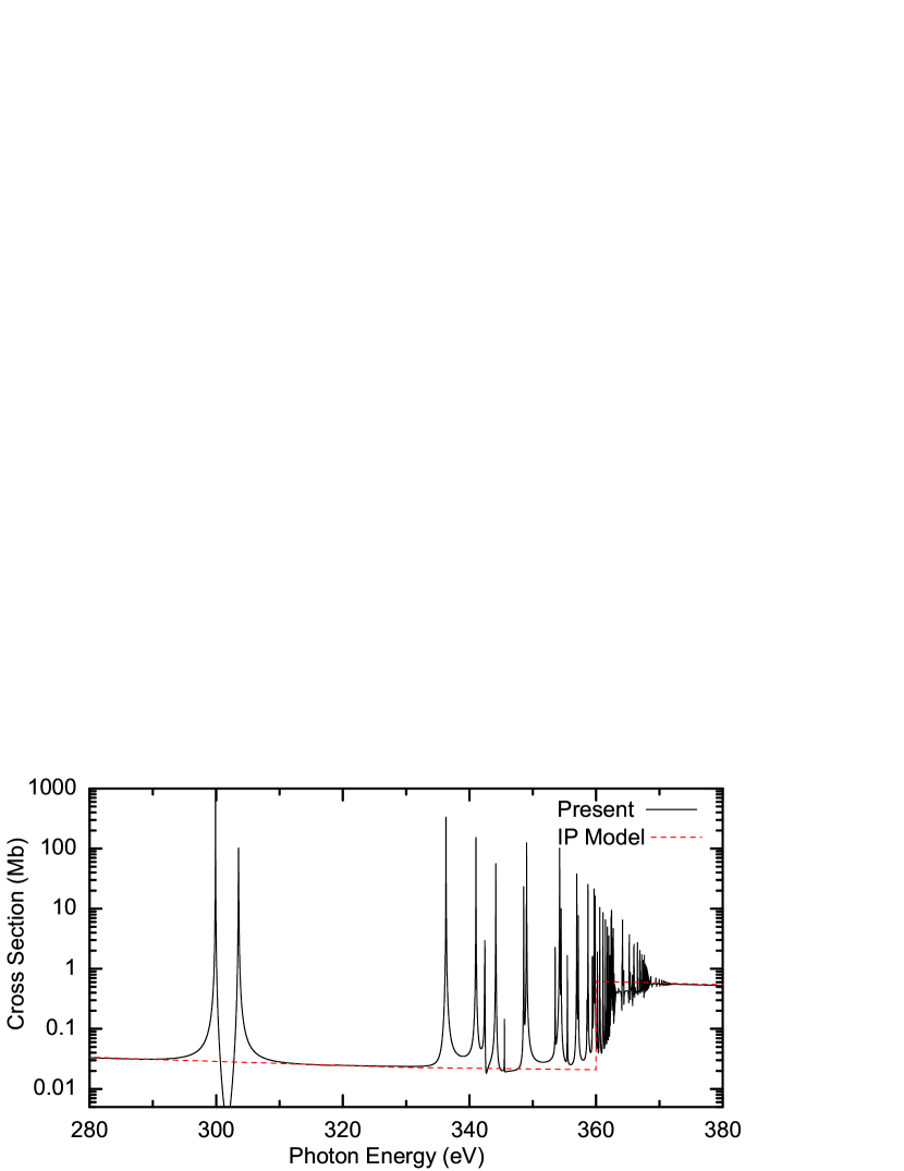
Figure 7: C IV photoabsorption cross sections.

The cross section for C IV is shown in Fig. 7. Here the resonances are given by $h\nu+1s^{2}2s\rightarrow 1s2snp$, and there is no spectator channel. Therefore, in order to be able to resolve the $n\rightarrow\infty$ narrowing resonances as threshold is approached, we artificially broadened the entire series with a spectator width of $\Gamma=0.027$ eV. This is less than the resolution of the ALS experimental measurements, which was given for C II (Schlachter et al., 2002), C III (Scully et al., 2005), and C IV (Müller et al., 2009) as $\Delta E\geq 0.046$ eV, or the astrophysical measurement we describe, which is given as $\Delta\lambda=0.023$ Å, or $\Delta E\approx 0.017$ eV for $E\approx 300$ eV.

4 The C K-Edge in the X-Ray Spectrum of Mkn 421

We have also compared our R-matrix photoabsorption cross sections with the absorption features in the C K-edge structure present in a Chandra LETG+HRC-S spectrum of the blazar Mkn 421. While the LETG+HRC-S instrument has a strong C K-edge feature arising from a polyimide filter approximately 2750 Å thick, there should be additional absorption signatures present from the line-of-sight absorption toward Mkn 421.

Chandra has observed Mkn 421 on several different occasions, but one observation made by the LETG+HRC-S on 2003 July 1-2 (ObsID 4149) caught the object in a particularly bright state and is of much higher quality. The observation and data are described in detail by Nicastro et al. (2005).

We retrieved standard pipeline-processed products from the Chandra archive and constructed effective areas for the overlapping spectral orders 1-10 using standard CIAO tasks. Subsequent analysis was performed using the Interactive Data Language-based Package for Interactive Analysis of Line Emission (PINTofALE; Kashyap & Drake, 2000). The adopted continuum model was optimized to the region around the C K-edge, ignoring the absorption edge structure. A power law continuum with photon index $\Gamma=2$ and interstellar medium (ISM) absorption corresponding to a neutral hydrogen column density of $N_{H}=1.5\times 10^{20}$ cm^-2 computed using the cross sections of Balucinska-Church & McCammon (1992) were adopted. These values are close (but not identical) to the values found by Nicastro et al. (2005); small differences can be ascribed to our optimization to the C K-edge region and to revisions in the instrument calibration between their and our analyses.

While we could obtain a good match to the observations over the continuum regions around the C K-edge, this model systematically underpredicted the data in the 42-44 Å range by about 5-15%. We ascribe this to uncertainty in the calibration—a notoriously difficult task for X-ray instruments in the vicinity of the C K-edge. We applied a smooth broad Gaussian-like correction to the effective area in order to ameliorate this effect. The resulting model fit is illustrated in Figure 9. While the fit is generally very good, there is a clear discrepancy near 43 Å. The Balucinska-Church & McCammon (1992) cross section for carbon is essentially that from the synthesis of Henke et al. (1982, 1993) combined with the C abundance of Anders & Ebihara (1982), and amounts to a simple step-function. We computed a new ISM absorption cross section replacing the neutral and ionized C cross sections with those from our R-Matrix computations. The division of carbon among different charge states was adjusted by eye to obtain a good match to the data. This was achieved with a mixture of 20% C I, 60% C II, and for illustrative purposes, 20% C III. The resulting model spectrum folded through the instrument response is also illustrated in Figure 9. There are no obvious signs of significant C IV absorption in the data.

We do not place great weight on the C ion ratios used for the fit: the instrument calibration would appear to require some revision before quantitative measurements can be made. However, we especially note two aspects of the results. Firstly, the C II resonance structure now provides a good match to the observations in the vicinity of 43 Å and we consider this a reliable detection of this species. To our knowledge, this represents the first X-ray identification of C II absorption in interstellar gas. Secondly, there is a weak absorption feature near 42.15 Å in the observed spectrum that is reasonably close to the C III $1s2s^{2}2p^{2}\,(^{1}P)$ resonance predicted by our R-Matrix calculations. The offset between the two is $\sim 0.05$ Å  or 0.35 eV. Based on the comparison of the R-matrix resonance energy and synchrotron observations illustrated in Figure 9, an offset of 0.35 eV is much too large to be associated with uncertainties in the predicted resonance position. Instead, it is possible that HRC-S imaging non-linearities could give rise to such a discrepancy. Line positions are generally expected to be better than 0.01-0.02 Å, but can occasionally be as far as 0.05 Å out of place. We stop short of identifying this absorption feature but draw attention to its possible interest for future study.

5 Summary and Conclusion

Photoabsorption features of carbon ions (C I-IV)) are studied using the R-matrix method, yielding, detailed information on the carbon K-shell photoabsorption cross section spectra. Furthermore, we computed photoabsorption cross sections for the additional C II, C III, and C IV isonuclear members, for which synchrotron-facility measurements at the ALS and theoretical studies already studied the lowest $1s\to 2p,3p$ resonance transitions. Our computed resonance positions were within about 0.5 eV of the measured values, and our strengths showed good agreement for some of the resonances but were significantly too large or small, compared to experiment, for certain strong resonances. These computed data are of particular importance for absorption studies of cosmic gas. In turn, a more accurate description of the interstellar absorption near the C K-edge in cosmic sources used as in-flight calibration standards should lead to refinements in the calibration of spectrometers such as the Chandra LETGS. Analysis of the LETGS spectrum of Mkn 421 has allowed us to identify interstellar absorption due to C II and estimate ion fractions of C I and C II for the first time using X-rays.

6 Acknowledgment

MFH, ShA, and TWG were supported in part by NASA APRA, NASA SHP SR&T, and Chandra Project grants. JJD was supported by NASA contract NAS8-39073 to the Chandra X-ray Center. BMMcL acknowledges support by the US National Science Foundation through a grant to ITAMP at the Harvard-Smithsonian Center for Astrophysics.

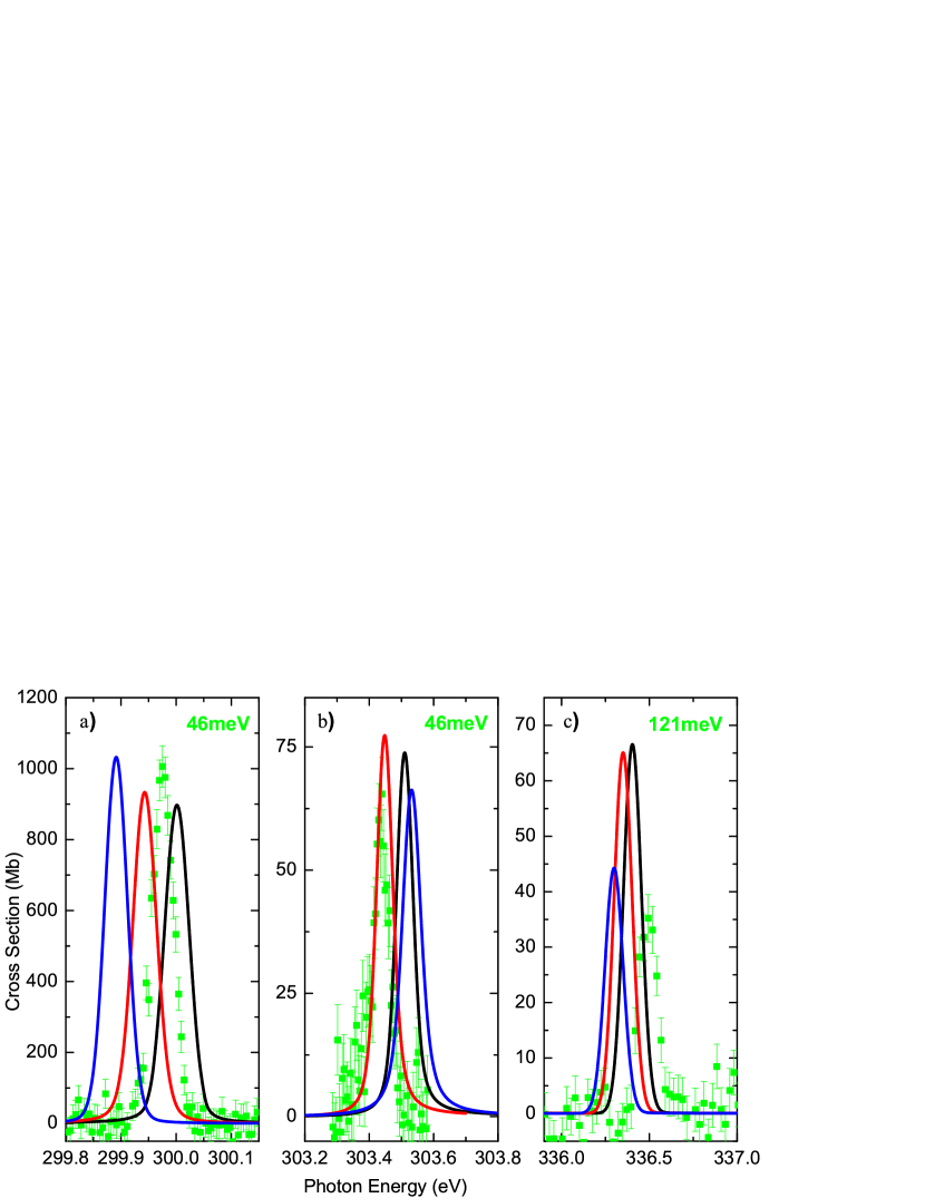
Figure 8: Present R-matrix cross section vs. experimental and earlier R-matrix results (Müller et al., 2009) for the $1s\to 2p,3p$ resonancs of C IV. The green data points represent the experimental data, the red and black curves show previous R-matrix results in IC- and LS-coupling, respectively, and the blue curve shows the present R-matrix results (all theoretical cross sections are convoluted with a FWHM Gaussian given by the experimental resolution). In a) and b), the $[1s(2s2p)^{3}P]^{2}P$ and $[1s(2s2p)^{1}P]^{2}P$ resonances, respectively, are measured with a spectral resolution of 46 meV, whereas for the $[1s(2s3p)^{3}P]^{2}P$ resonance in c) , the resolution is 121 meV.

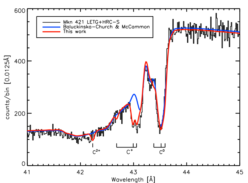
Figure 9: The carbon K-edge region of the X-ray spectrum of the bright blazar Mkn 421 observed by the Chandra LETG+HRC-S. The edge absorption is predominantly due to the polyimide UV-optical/ion blocking filter on the HRC-S instrument, although ISM absorption contributions are also present. Two fits to a power-law continuum model with photon index $\Gamma=2.0$, absorbed by an intervening ISM corresponding to a neutral H column density of $1.5\times 1020$ cm^-2, are shown. These differ significantly only in the carbon cross-sections employed: the neutral C I cross-section of Balucinska-Church & McCammon (1992); and C I, C II and C III cross-sections reported here. In the latter case, the C ion fractions were 20% C I, 60 % C II and 20% C III. The effect of the C II resonances are clearly visible in the vicinity of 43 Å.

Table 1: Energies (in Rydbergs) of the C II target states and the C I ground state. The $1s2s^{2}2p^{2}\,(^{4}P)$ energy of 20.9133 Ryd relative to the $1s^{2}2s^{2}2p\,(^{2}P)$ ground state of C II corresponds to a K-shell threshold energy of 296.098 eV relative to the C I ground state, which compares favorably to the experimental value of $296.07\pm 0.2$ eV Bruch et al. (1985).

State	R-matrix	NIST
$1s^{2}2s^{2}2p^{2}\,(^{3}P)$	$-0.8493$	$-0.8277$
$1s^{2}2s^{2}2p\,(^{2}P)$	$0.0000$	$0.0000$
$1s^{2}2s2p^{2}\,(^{4}P)$	$0.3814$	$0.3922$
$1s^{2}2s2p^{2}\,(^{2}D)$	$0.7128$	$0.6828$
$1s^{2}2s2p^{2}\,(^{2}S)$	$0.9850$	$0.8793$
$1s^{2}2s2p^{2}\,(^{2}P)$	$1.0450$	$1.0083$
$1s^{2}2p^{3}\,(^{4}S)$	$1.3104$	$1.2942$
$1s^{2}2p^{3}\,(^{2}D)$	$1.4311$	$1.3711$
$1s^{2}2p^{3}\,(^{2}P)$	$1.6792$	$1.5377$
$1s2s^{2}2p^{2}\,(^{4}P)$	$20.9133$
$1s2s^{2}2p^{2}\,(^{2}D)$	$21.1651$
$1s2s^{2}2p^{2}\,(^{2}P)$	$21.1899$
$1s2s^{2}2p^{2}\,(^{2}S)$	$21.3351$
$1s2s(^{1}S)2p^{3}\,(^{4}S)$	$21.4753$
$1s2s(^{3}S)2p^{3}\,(^{4}D)$	$21.5097$
$1s2s(^{3}S)2p^{3}\,(^{4}P)$	$21.6968$
$1s2s(^{1}S)2p^{3}\,(^{2}D)$	$21.8446$
$1s2s(^{1}S)2p^{3}\,(^{2}P)$	$22.0355$
$1s2s(^{3}S)2p^{3}\,(^{4}S)$	$22.0847$
$1s2s(^{3}S)2p^{3}\,(^{2}D)$	$22.1103$
$1s2s(^{3}S)2p^{3}\,(^{2}S)$	$22.2898$
$1s2s(^{3}S)2p^{3}\,(^{2}P)$	$22.3180$
$1s2p^{4}\,(^{4}P)$	$22.4901$
$1s2p^{4}\,(^{2}D)$	$22.6795$
$1s2p^{4}\,(^{2}P)$	$22.7300$
$1s2p^{4}\,(^{2}S)$	$23.0860$

Table 2: Energies (in Rydbergs) of the C III target states and the C II ground state.

State	R-matrix	NIST
$1s^{2}2s^{2}2p\,(^{2}P)$	$-1.7977$	$-1.7921$
$1s^{2}2s^{2}\,(^{1}S)$	$0.0000$	$0.0000$
$1s^{2}2s2p\,(^{3}P)$	$0.4745$	$0.4777$
$1s^{2}2s2p\,(^{1}P)$	$0.9570$	$0.9327$
$1s^{2}2p^{2}\,(^{3}P)$	$1.2649$	$1.2528$
$1s^{2}2p^{2}\,(^{1}D)$	$1.3630$	$1.3293$
$1s^{2}2p^{2}\,(^{1}S)$	$1.7881$	$1.6632$
$1s2s^{2}2p\,(^{3}P)$	$21.3622$
$1s2s^{2}2p\,(^{1}P)$	$21.5849$
$1s2s(^{1}S)2p^{2}\,(^{3}P)$	$21.9689$
$1s2s(^{3}S)2p^{2}\,(^{3}D)$	$21.9997$
$1s2s(^{3}S)2p^{2}\,(^{1}D)$	$22.3201$
$1s2s(^{3}S)2p^{2}\,(^{3}S)$	$22.3269$
$1s2s(^{3}S)2p^{2}\,(^{3}P)$	$22.4088$
$1s2s(^{3}S)2p^{2}\,(^{1}P)$	$22.5674$
$1s2s(^{1}S)2p^{2}\,(^{1}S)$	$22.6511$
$1s2p^{3}\,(^{3}D)$	$22.6802$
$1s2p^{3}\,(^{3}S)$	$22.7780$
$1s2p^{3}\,(^{1}D)$	$22.8708$
$1s2p^{3}\,(^{3}P)$	$22.9926$
$1s2p^{3}\,(^{1}P)$	$23.1865$

Table 3: Energies (in Rydbergs) of the C IV target states and the C III ground state.

State	R-matrix	NIST
$1s^{2}2s^{2}\,(^{1}S)$	$-3.5264$	$-3.5197$
$1s^{2}2s\,(^{2}S)$	$0.0000$	$0.0000$
$1s^{2}2p\,(^{2}P)$	$0.5903$	$0.5883$
$1s2s^{2}\,(^{2}S)$	$21.3887$
$1s2s(^{1}S)2p\,(^{2}P)$	$22.0009$
$1s2s(^{3}S)2p\,(^{2}P)$	$22.2608$
$1s2p^{2}\,(^{2}D)$	$22.4955$
$1s2p^{2}\,(^{2}P)$	$22.5767$
$1s2p^{2}\,(^{2}S)$	$23.0266$

Table 4: Energies (in Rydbergs) of the C V target states and the C IV ground state.

State	R-matrix	NIST
$1s^{2}2s\,(^{2}S)$	$-4.7402$	-4.7402
$1s^{2}\,(^{1}S)$	$0.0000$	0.0000
$1s2s\,(^{3}S)$	$21.9670$	21.9731
$1s2s\,(^{1}S)$	$22.3662$	22.3718
$1s2p\,(^{3}P)$	$22.3673$	22.3737
$1s2p\,(^{1}P)$	$22.6236$	22.6302

Table 5: R-matrix Auger widths (in eV) for the 17 C II autoionizing target states above the K-shell threshold (see Table 1). Also shown are level-averaged MBCP (Hasoğlu et al., 2006) and level-averaged MCDF (Chen, 1985) widths.

	State		R-matrix		MCBP		MCDF
1	$1s2s^{2}2p^{2}\,(^{4}P)$		$6.45E-02$		$8.61E-02$		$6.68E-02$
2	$1s2s^{2}2p^{2}\,(^{2}D)$		$9.14E-02$		$1.16E-01$		$8.62E-02$
3	$1s2s^{2}2p^{2}\,(^{2}P)$		$4.93E-02$		$5.19E-02$		$4.75E-02$
4	$1s2s^{2}2p^{2}\,(^{2}S)$		$8.65E-02$		$1.02E-01$		$1.49E-04$
5	$1s2s(^{1}S)2p^{3}\,(^{4}S)$		$1.55E-02$		$2.06E-02$		$5.86E-02$
6	$1s2s(^{3}S)2p^{3}\,(^{4}D)$		$4.60E-02$		$6.42E-02$		$4.77E-02$
7	$1s2s(^{3}S)2p^{3}\,(^{4}P)$		$3.56E-02$		$4.87E-02$		$3.73E-02$
8	$1s2s(^{1}S)2p^{3}\,(^{2}D)$		$7.21E-02$		$9.64E-02$		$9.08E-02$
9	$1s2s(^{1}S)2p^{3}\,(^{2}P)$		$6.42E-02$		$7.77E-02$		$8.01E-02$
10	$1s2s(^{3}S)2p^{3}\,(^{4}S)$		$4.57E-02$		$7.15E-02$		$2.49E-02$
11	$1s2s(^{3}S)2p^{3}\,(^{2}D)$		$7.78E-02$		$1.18E-01$		$8.23E-02$
12	$1s2s(^{3}S)2p^{3}\,(^{2}S)$		$1.49E-02$		$1.25E-02$		$8.89E-03$
13	$1s2s(^{3}S)2p^{3}\,(^{2}P)$		$6.56E-02$		$1.01E-01$		$7.13E-02$
14	$1s2p^{4}\,(^{4}P)$		$3.89E-03$		$6.83E-02$		$5.18E-02$
15	$1s2p^{4}\,(^{2}D)$		$7.24E-02$		$1.08E-01$		$8.16E-02$
16	$1s2p^{4}\,(^{2}P)$		$4.60E-02$		$6.69E-02$		$5.03E-02$
17	$1s2p^{4}\,(^{2}S)$		$4.90E-02$		$1.36E-01$		$5.56E-02$

Table 6: R-matrix Auger widths (in eV) for the C III autoionizing target states above the K-shell threshold (see Table 2). Also shown are level-averaged MBCP (Gorczyca et al., 2003) and level-averaged MCDF (Chen, 1985) widths.

	State		R-matrixa		MCBP		MCDF
1	$1s2s^{2}2p\,(^{3}P)$		$7.18E-02$		$7.93E-02$		$6.72E-02$
2	$1s2s^{2}2p\,(^{1}P)$		$5.46E-02$		$5.30E-02$		$4.76E-02$
3	$1s2s(^{1}S)2p^{2}\,(^{3}P)$		$1.10E-02$		$1.38E-02$		$2.47E-02$
4	$1s2s(^{3}S)2p^{2}\,(^{3}D)$		$4.76E-02$		$5.17E-02$		$4.29E-02$
5	$1s2s(^{3}S)2p^{2}\,(^{1}D)$		$9.07E-02$		$1.14E-01$		$1.13E-01$
6	$1s2s(^{3}S)2p^{2}\,(^{3}S)$		$2.61E-02$		$2.39E-02$		$2.17E-02$
7	$1s2s(^{3}S)2p^{2}\,(^{3}P)$		$4.64E-02$		$5.92E-02$		$4.91E-02$
8	$1s2s(^{3}S)2p^{2}\,(^{1}P)$		$1.70E-02$		$1.17E-02$		$7.96E-03$
9	$1s2s(^{1}S)2p^{2}\,(^{1}S)$		$7.46E-02$		$7.98E-02$		$8.36E-02$
10	$1s2p^{3}\,(^{3}D)$		$5.76E-02$		$7.15E-02$		$6.08E-02$
11	$1s2p^{3}\,(^{3}S)$		$-$		$-$		$1.17E-06$
12	$1s2p^{3}\,(^{1}D)$		$5.99E-02$		$7.19E-02$		$6.02E-02$
13	$1s2p^{3}\,(^{3}P)$		$3.56E-02$		$4.19E-02$		$3.67E-02$
14	$1s2p^{3}\,(^{1}P)$		$3.60E-02$		$3.90E-02$		$3.53E-02$

Table 7: R-matrix Auger widths (in eV) for the C IV autoionizing target states above the K-shell threshold (see Table 3). Also shown are level-averaged MBCP (Gorczyca et al., 2006) and level-averaged MCDF (Chen, 1985) widths.

	State		R-matrix		MCBP
1	$1s2s^{2}\,(^{2}S)$		$6.99E-02$		$7.12E-02$
2	$1s2s(^{1}S)2p\,(^{2}P)$		$3.95E-03$
3	$1s2s(^{3}S)2p\,(^{2}P)$		$3.64E-02$
4	$1s2p^{2}\,(^{2}D)$		$5.48E-02$		$6.07E-02$
5	$1s2p^{2}\,(^{2}P)$
6	$1s2p^{2}\,(^{2}S)$		$8.76E-03$		$5.22E-03$

References

- Anders & Ebihara (1982) Anders, E., & Ebihara, M. 1982, Geochim. Cosmochim. Acta, 46, 2363
- Badnell et al. (1997) Badnell, N. R., Petrini, D., & Stocia, S. 1997, J. Phys. B: At. Mol. & Opt., 30, L665
- Balucinska-Church & McCammon (1992) Balucinska-Church, M., & McCammon, D. 1992, ApJ, 400, 699
- Berrington et al. (1995) Berrington, K. A., Eissner, W. B., & Norrington, P. H. 1995, Comput. Phys. Communi., 92, 290
- Bisgaard et al. (1978) Bisgaard, P., Bruch, Dahl, P., Fastrup, B., & Rødbro, M. 1978, Phys. Scr., 17, 49
- Bruch et al. (1985) Bruch, R., Luken, W. L., Culberson, J. C., & Chung, K. T. 1985, Phys. Rev. A, 31, 503
- Burke & Berrington (1993) Burke, P. G., & Berrington, K. A. 1993, Atomic and molecular processes : an R-matrix approach (Bristol; Philadelphia: Institute of Physics Pub.)
- Carroll & Kennedy (1977) Carroll, P. K., & Kennedy, E. T. 1977, Phys. Rev. Lett., 38, 1068
- Chen (1985) Chen, M. H. 1985, Phys. Rev. A, 31, 1449
- Coreno et al. (1999) Coreno, M., Avaldi, L., Camilloni, R., Prince, K. C., de Simone, M., Karvonen, J., Colle, R., & Simonucci, S. 1999, Phys. Rev. A, 59, 2494
- de Vries et al. (2003) de Vries, C. P., den Herder, J. W., Kaastra, J. S., Paerels, F. B., den Boggende, A. J., & Rasmussen, A. P. 2003, A&A, 404, 959
- Fischer (1977) Froese Fischer, C. F. 1977, The Hartree-Fock method for atoms : a numerical approach (New York: Wiley)
- Fischer et al. (1997) Fischer, C. F., Brage, T., & Jönsson, P. 1997, Computational atomic structure : an MCHF approach (Bristol, UK; Philadelphia, Penn: Institute of Physics Publ.)
- Fischer (1991) Fischer, C. F. 1991, Comput. Phys. Communi., 64, 369
- Garcia et al. (2005) Garcia, J., Mendoza, C., Bautista, M. A., Gorczyca, T. W., Kallman, T. R., & Palmeri, P. 2005, The Astrophysical Journal Supplement Series, 158, 68
- Gorczyca & Robicheaux (1999) Gorczyca, T. W., & Robicheaux, F. 1999, Phys. Rev. A, 60, 1216
- Gorczyca (2000) Gorczyca, T. W. 2000, Phys. Rev. A, 61, 024702
- Gorczyca & McLaughlin (2000) Gorczyca, T. W., & McLaughlin, B. M. 2000, Journal of Physics B: Atomic Molecular Physics, 33, L859
- Gorczyca et al. (2003) Gorczyca, T. W., Kodituwakku, C. N., Korista, K. T., Zatsarinny, O., Badnell, N. R., Behar, E., Chen, M. H., & Savin, D. W. 2003, ApJ, 592, 636
- Gorczyca et al. (2006) Gorczyca, T. W., Dumitriu, I., Hasoğlu, M. F., Korista, K. T., Badnell, N. R., Savin, D. W., & Manson, S. T. 2006, ApJ, 638, L121
- Hasoğlu et al. (2006) Hasoglu, M. F., Gorczyca, T. W., Korista, K. T., Manson, S. T., Badnell, N. R., & Savin, D. W. 2006, ApJ, 649, L149
- Henke et al. (1982) Henke, B. L., Lee, P., Tanaka, T. J., Shimabukuro, R. L., & Fujikawa, B. K. 1982, Atomic Data and Nuclear Data Tables, 27, 1
- Henke et al. (1993) Henke, B. L., Gullikson, E. M., & Davis, J. C. 1993, At. Data Nucl. Data Tables, 54, 181
- Jannitti et al. (1990) Jannitti, E., Nicolosi, P., & Tondello, G. 1990, Phys. Scr., 41, 458
- Juett et al. (2004) Juett, A. M., Schulz, N. S., & Chakrabarty, D. 2004, ApJ, 612, 308
- Juett et al. (2006) Juett, A. M., Schulz, N. S., Chakrabarty, D., & Gorczyca, T. W. 2006, ApJ, 648, 1066
- Kaastra et al. (2009) Kaastra, J. S., de Vries, C. P., Costantini, E., & den Herder, J. W. A. 2009, A&A, 497, 291
- Kashyap & Drake (2000) Kashyap, V., & Drake, J. J. 2000, Bulletin of the Astronomical Society of India, 28, 475
- McLaughlin (2001) McLaughlin B M 2001 Spectroscopic Challenges of Photoionized Plasma (ASP Con. Series 113 vol 247) ed G Ferland and D W Savin (San Francisco, CA: Astronomical Society of the Pacific) p 87
- Müller et al. (2009) Müller, A., et al. 2009, J. Phys B: At. Mol. & Opt. Phys., 42, 235602
- Ness et al. (2007) Ness, J.-U., et al. 2007, ApJ, 665, 1334
- Nicastro et al. (2005) Nicastro, F., et al. 2005, ApJ, 629, 700
- Nicolosi et al. (1991) Nicolosi, P., Jannitti, E., & Tondello, G. 1991, J. de Physique IV., Colloque C1, supplement au Journal de Physique II, 89-98
- O’Sullivan et al. (1996) O’Sullivan, G., McGuinness, C., Costello, J.T., Kennedy, E. T., & Weinmann, B. 1996, Phys. Rev. A, 53, 3211
- Paerels et al. (2001) Paerels, F., et al. 2001, ApJ, 546, 338
- Petrini & da Silva (1999) Petrini, D., & da Silva, E. P. 1999, A&A, 348, 659
- Reilman & Manson (1979) Reilman, R. F., & Manson, S. T. 1979, ApJS, 40, 815
- Schattenburg & Canizares (1986) Schattenburg, M. L., & Canizares, C. R. 1986, ApJ, 301, 759
- Schlachter et al. (2002) Schlachter, A. S., et al. 2002, J. Phys. B: At. Mol. Opt. Phys., 37, L103
- Scully et al. (2005) Scully, S. W. J., et al. 2005, J. Phys. B: At. Mol. Opt. Phys., 38, 1967
- Smith (1960) Smith, Felix T. 1960, Phys. Rev. A, 118, 349
- Takei et al. (2002) Takei, Y., Fujimoto, R., Mitsuda, K., & Onaka, T. 2002, ApJ, 581, 307
- Ueda et al. (2005) Ueda, Y., Mitsuda, K., Murakami, H., & Matsushita, K. 2005, ApJ, 620, 274
- Verner et al. (1993) Verner, D. A. et al. 1993, At. Data Nucl. Data Tables, 55, 233
- Verner & Yakovlev (1995) Verner, D. A., & Yakovlev, D. G. 1995, A&AS, 109, 125
- Yao & Wang (2006) Yao, Y., & Wang, Q. D. 2006, ApJ, 641, 930
- Yao et al. (2009) Yao, Y., Schulz, N. S., Gu, M. F., Nowak, M. A., & Canizares, C. R. 2009, ApJ, 696, 1418
- Yeh (1993) Yeh, J. 1993, Atomic Calculation of Photoionization Cross-Sections and Asymmetry Parameters, (New York : Gordon & Breach)