The core helium flash revisited

Abstract

Context. Degenerate ignition of helium in low-mass stars at the end of the red giant branch phase leads to dynamic convection in their helium cores. One-dimensional (1D) stellar modeling of this intrinsically multi-dimensional dynamic event is likely to be inadequate. Previous hydrodynamic simulations imply that the single convection zone in the helium core of metal-rich Pop I stars grows during the flash on a dynamic timescale. This may lead to hydrogen injection into the core, and a double convection zone structure as known from one-dimensional core helium flash simulations of low-mass Pop III stars.

Aims. We perform hydrodynamic simulations of the core helium flash in two and three dimensions to better constrain the nature of these events. To this end we study the hydrodynamics of convection within the helium cores of a 1.25 M_⊙ metal-rich Pop I star (Z=0.02), and a 0.85 M_⊙ metal-free Pop III star (Z=0) near the peak of the flash. These models possess single and double convection zones, respectively.

Methods. We use 1D stellar models of the core helium flash computed with state-of-the-art stellar evolution codes as initial models for our multidimensional hydrodynamic study, and simulate the evolution of these models with the Riemann solver based hydrodynamics code Herakles which integrates the Euler equations coupled with source terms corresponding to gravity and nuclear burning.

Results. The hydrodynamic simulation of the Pop I model involving a single convection zone covers 27 hours of stellar evolution, while the first hydrodynamic simulations of a double convection zone, in the Pop III model, span 1.8 hours of stellar life. We find differences between the predictions of mixing length theory and our hydrodynamic simulations. The simulation of the single convection zone in the Pop I model shows a strong growth of the size of the convection zone due to turbulent entrainment. Hence we predict that for the Pop I model a hydrogen injection phase (i.e., hydrogen injection into the helium core) will commence after about 23 days, which should eventually lead to a double convection zone structure known from 1D stellar modeling of low-mass Pop III stars. Our two and three-dimensional hydrodynamic simulations of the double (Pop III) convection zone model show that the velocity field in the convection zones is different from that predicted by stellar evolutionary calculations. The simulations suggest that the double convection zone decays quickly, the flow eventually being dominated by internal gravity waves.

1 Introduction

Runaway nuclear burning of helium in the core of low mass red giant stars leads to convective mixing and burning on dynamic time scales. One dimensional evolutionary simulations (which assume time scales much longer than the dynamical ones) may miss key features of this rapid phase that could have significant effects on the further evolution of the stars. Furthermore, 1D hydrodynamical simulations of this intrinsically multi-dimensional event is likely to be inadequate.

Our previous hydrodynamic simulations (Mocák et al. 2008, 2009) imply that a $1.25\,$M_⊙ solar-like star can experience injection of hydrogen into its helium core during the canonical core helium flash near its peak. Hydrogen injection results from the growth of the convection zone (which is sustained by helium burning) due to turbulent entrainment on a dynamic timescale (Meakin & Arnett 2007), and probably occurs for all low-mass Pop I stars, as the properties of their cores are similar at the peak of the core helium flash (Sweigart & Gross 1978). An obvious consequence of this scenario is that the convection zones are enlarged in these stars. Whether they fail to dredge up nuclear ash to the atmosphere shortly after the flash is still unclear. However, such a dredge up could explain the Al-Mg anticorrelation found in red giants at the tip of the red giant branch (Shetrone 1996a, b; Yong et al. 2006). In 1D simulations one has to manipulate the properties of the core helium flash to achieve such a dredge up, e.g., by changing the ignition position of the helium in the core (Paczynski & Tremaine 1977) or by forcing inward mixing of hydrogen (Fujimoto et al. 1999).

Canonical (1D) stellar evolution calculations predict hydrogen injection during the core helium flash and subsequent dredge-up of nuclear ashes to the atmosphere only for Pop III and extremely metal-poor (EMP; with intrinsic metallicities [Fe/H] $\lesssim-4$) stars. This is a promising scenario for explaining the peculiar abundances of carbon and nitrogen observed in Galactic EMP Halo stars (Campbell & Lattanzio 2008). If these stars are assumed to be polluted by accretion of CNO-rich interstellar matter they will possibly experience hydrogen injection but no subsequent dredge-up, because a large CNO metallicitiy (as compared to the intrinsic [Fe/H] metallicity) in the stellar envelope influences the ignition site of the first major core helium flash, and thereby the occurrence of the dredge-up (Hollowell et al. 1990). The helium abundance adopted in the stellar models also seems to influence the process of hydrogen injection itself as shown by Schlattl et al. (2001), while the same authors find that the injection process seems to be independent of the assumed convection model.

Stellar models with a higher intrinsic metallicity, i.e., [Fe/H] $>-4$, do not inject hydrogen into the helium core, and consequently there is also no dredge-up of CNO-rich nuclear ashes to the atmosphere (Fujimoto et al. 1990; Hollowell et al. 1990; Campbell & Lattanzio 2008). Whether this is the final answer remains unclear, however, as Fujimoto et al. (1999) with his semi-analytic study and a postulated hydrogen injection followed by a dredge-up could show that such a scenario can explain some peculiarities observed in the spectra of red-giant stars (related to CNO elements and ²⁴Mg) with metallicities as large as [Fe/H] $\lesssim-1$.

There exist two main reasons why hydrogen injection episodes occur only in Pop III and EMP stars: ($i$) these stars possess a flatter entropy gradient in the hydrogen burning shell, and ($ii$) they ignite helium far off center, relatively close to the hydrogen-rich envelope (Fujimoto et al. 1990). However, Pop II and Pop I stars could also mix hydrogen into the helium core during the core helium flash

• if the flash was more violent, and thus the helium convection zone wider (Despain & Scalo 1976; Despain 1981). This scenario is disfavored by the facts that the flash is less violent in stars with higher metallicity as less energy is needed to lift the degeneracy of the less massive cores (Sweigart & Gross 1978), and that helium ignition occurs at smaller densities (Fujimoto et al. 1990),

• or if the entropy gradient between the hydrogen and helium burning shell was sufficiently shallow (Iben 1976; Fujimoto 1977). A small entropy gradient would allow the convective shell in the helium core to reach the hydrogen layers even though the flash itself would not be very violent. This scenario is also disfavored as solutions to the stellar structure equations are robust with many different groups getting very similar results i.e., no hydrogen injection (Fujimoto et al. 1990; Hollowell et al. 1990; Campbell & Lattanzio 2008)

• or if a growth of the helium convection zone through turbulent entrainment at the convective boundaries (Mocák et al. 2008, 2009) could be sustained for a sufficiently long period of time.

A hydrogen injection phase also occurs in low-mass metal deficient stars on the asymptotic giant branch (AGB) at the beginning of the thermally pulsing stage (TPAGB) .

Hydrogen injection is found to occur in more massive stars ($M\gtrsim 1.3\,$M_⊙ ) with low metallicity during the TPAGB (Chieffi et al. 2001; Siess et al. 2002; Iwamoto et al. 2004), in “Late Hot Flasher” stars experiencing strong mass loss on the RGB (Brown et al. 2001; Cassisi et al. 2003), and in H-deficient post AGB (PAGB) stars. These events are referred to with various names in the literature. Here we use the nomenclature “dual flashes” (Campbell & Lattanzio 2008), since they all have in common simultaneous hydrogen and helium flashes.

Dual flash events often lead to a splitting of the single helium convection zone (HeCZ) into two parts (double convection zone): one sustained by helium burning, and a second one by hydrogen burning via CNO cycles (Fig. 1). Double convection zones are structures which are commonly encountered in stellar models, but their hydrodynamic properties have so far only been studied for the oxygen and carbon burning shell of a $23\,$M_⊙ star by Meakin & Arnett (2006).

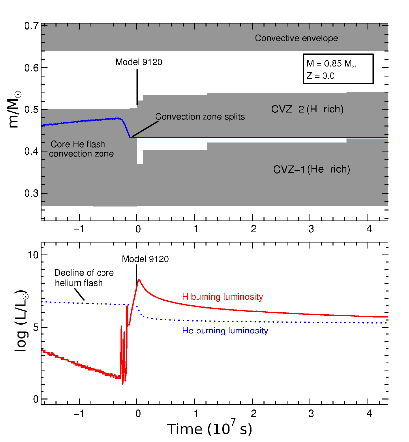
Figure 1: Upper panel: Kippenhahn diagram of a stellar evolutionary calculation during the core helium flash of a $0.85\,$M_⊙ Pop III star with convection zones sustained by helium (He-rich) and hydrogen (H-rich) or CNO burning (grey shaded regions, except for the convective envelope). The border between the helium and hydrogen rich layers is given by the solid blue curve. The location of the initial model SC (model number 9120) - black vertical line. Lower panel: the temporal evolution of the helium (dotted-blue) and hydrogen (solid-red) luminosity as a function of time.

In the following we describe two-dimensional (2D) and three-dimensional (3D) hydrodynamic simulations of a helium core during the core helium flash with a single convection zone (Pop I; in 3D only) and a double convection zone (Pop III, in 2D and 3D), respectively. Previous studies have indicated that there is a strong interaction between the adjacent shells of a double convection zone by internal gravity waves (Meakin & Arnett 2006).

We introduce the stellar models used as input for our hydrodynamic simulations in Sect. 2, briefly discuss the physics included in our simulations in Sect. 3, and give a short description of our hydrodynamics code and the computational setup in Sect. 4. Subsequently, we present and compare the results of our 2D and 3D hydrodynamic simulations in Sect. 5. In particular, we discuss turbulent entrainment at the convective boundaries for our single convection zone model, the temporal evolution of its kinetic energy density, and how our results compare with the predictions of mixing-length theory (MLT). We proceed similarly for our hydrodynamic double convection zone model, except for turbulent entrainment for reasons which become clear later. Finally, a summary of our findings is given in Sect. 6.

2 Physical Conditions and Initial Data

Our initial helium core models (Tab. 1) with single and double convection zones (models M and SC, respectively) are obtained from 1D stellar evolutionary calculations of a Pop I star (Z=0.02) with a mass of $1.25\,$M_⊙ , and a Pop III star (Z=0) with a mass of 0.85 M_⊙ , , respectively. Both models are characterized by an off-center helium ignition which results in convection zones characterized by a temperature gradient close to the adiabatic one above the helium burning source.

The helium cores of both models are composed of a gas which is almost completely ionized, as the ionization potentials of both He and He⁺ ($E_{B}\sim 24.7\,$eV and $E_{B}\sim 54.4\,$eV, respectively) are very small compared to the thermal energy, i.e.,

$$\frac{E_{B}}{k_{B}T}<10^{-2}\,,$$ (1)

where $k_{B}$ is Boltzmann’s constant, and $T>4.7\times 10^{7}\,$K ($T>1.7\times 10^{7}\,$K) holds for the temperature inside the helium core of model M (SC) which has a radius $r\sim 1.9\times 10^{9}\,$cm ($r\sim 5.4\times 10^{9}\,$cm ).

In the central part of the models (beneath the convection zones) the electron density is so high that the gas is highly degenerate. On the other hand, the density of electrons in the single and double convection zone is much lower due to a strong expansion that occurred a little earlier in the evolution. Thus, the degeneracy has been lifted in the convection zones, i.e., the ratio of the Fermi energy $E_{F,E}$ of the electrons (Weiss et al. 2004) and their typical thermal energy is small,

$$\frac{E_{F,E}}{k_{B}T}\sim 2.47\,\,\,\,\,(0.14)$$ (2)

where $E_{F,E}\sim 4.1\times 10^{-8}\mbox{\ erg }$ ($E_{F,E}\sim 1.2\times 10^{-9}\mbox{\ erg }$ ) in the middle of the convection zone of model M (SC) at a radius $r\sim 7\times 10^{8}$ cm ($r\sim 3.3\times 10^{9}\,$cm).

The ions can be described as an ideal, non-relativistic Boltzmann gas, because the ratio of their Fermi energy $E_{F,I}$ and their typical thermal energy is small,

$$\frac{E_{F,I}}{k_{B}T}\sim 2\times 10^{-4}\,\,\,\,\,(1\times 10^{-5})$$ (3)

where $E_{F,I}\sim 3.4\times 10^{-12}\mbox{\ erg }$ ($E_{F,I}\sim 1\times 10^{-13}\mbox{\ erg }$ ) in the middle of the convection zone of model M (SC) at a radius $r\sim 7\times 10^{8}\mbox{\ cm}$ ($r\sim 3.3\times 10^{9}\,$cm). Coulomb forces between the ions are negligible, too, as the Coulomb energy corresponding to the mean ion-ion distance is less than 30% (10%) of the thermal energy of the ions for model M (SC) in the middle of the convection zone.

Table 1: Some properties of the initial models M & SC: Total mass $M$, stellar population, metal content $Z$, mass $M_{He}$ and radius $R_{He}$ of the helium core ($X(^{4}He)>0.98$), ratio of the binding energy of the electrons $E_{B}$ in the helium core and of their thermal energy $k_{B}T$, ratio of the Coulomb and thermal energy of the ions $\Gamma_{cnv}$, electron degeneracy parameter in the convection zone $\Psi_{cnv}$, nuclear energy production rate due to helium $L_{He}$ and hydrogen $L_{He}$ burning, temperature maximum $T_{max}$, and radius $r_{max}$ and density $\rho_{max}$ at the temperature maximum.

Model	$M$	Pop.	$Z$	$M_{He}$	$R_{He}$	EB/kBT	$\Gamma_{cnv}$	$\Psi_{cnv}$	$L_{He}$	$L_{H}$	$T_{max}$	$r_{max}$	$\rho_{max}$
	$[\mbox{M${}_{\odot}$\,}]$			$[\mbox{M${}_{\odot}$\,}]$	$[10^{9}\mbox{\ cm}]$				$[10^{9}\mbox{$L_{\odot}$}]$	$[10^{9}\mbox{$L_{\odot}$}]$	$[10^{8}\mbox{\ K}]$	$[10^{8}\mbox{\ cm}]$	$[10^{5}\mbox{\ g cm${}^{-3}$}]$
M	$1.25$	I	$0.02$	$0.47$	$1.91$	$<$ 0.006	0.3	5	$1.03$	$10^{-6}$	$1.70$	$4.71$	$3.44$
SC	0.85	III	$0.00$	$0.5$	$5.45$	$<$ 0.016	0.1	-2	$0.004$	0.07	$2.04$	$11.$	$0.08$

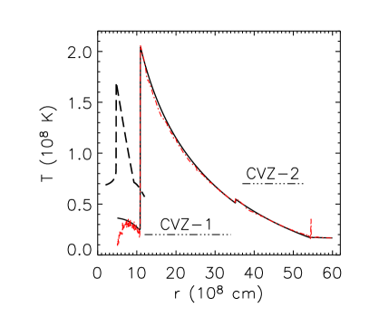
Figure 2: Left: Temperature distribution in the helium core in model M (long-dashed), and in model SC (solid) with its stabilized counterpart (dash-dotted red), respectively. The two parts of the double convection zone present in model SC are denoted by CVZ-1 and CVZ-2, respectively. Right: Entropy distribution of model M (solid) and model SC (long-dashed), respectively.

Convection may become turbulent showing random spatial and temporal fluctuations. This can be characterized by the dimensionless Reynolds number $R_{e}$ (Landau & Lifshitz 1966) which is basically the ratio of inertial to viscous forces. The turbulent regime is entered once $R_{e}$ exceeds a certain critical value $R_{crit}$, typically being of the order of $10^{3}$, at which small fluctuations in the flow are no longer damped. We estimate that the Reynolds numbers in the central convection zones of our models are

$$R_{e}\sim\frac{v\cdot l\cdot\rho}{\eta}\sim 10^{14}\,\,\,\,\,(10^{14})$$ (4)

where $\rho\sim 10^{5}\mbox{\ g cm${}^{-3}$}$ ($\rho\sim 10^{3}\mbox{\ g cm${}^{-3}$}$), $l\sim 10^{8}\mbox{\ cm}$ ($l\sim 10^{9}\mbox{\ cm}$), $v\sim 10^{6}\mbox{\ cm s${}^{-1}$}$ ($v\sim 10^{5}\mbox{\ cm s${}^{-1}$}$), and $\eta\sim 10^{5}\mbox{$\mbox{\ g}\mbox{\ cm}^{-1}\mbox{\ s}^{-1}$}$ ($\eta\sim 10^{3}\mbox{$\mbox{\ g}\mbox{\ cm}^{-1}\mbox{\ s}^{-1}$}$) are the typical densities, lengths, velocities, and viscosities of the convective flow in model M (SC) as predicted by stellar evolutionary calculations. These values imply that the flow is highly turbulent, which leads to complications when trying to simulate such flows, as turbulence is an intrinsically three-dimensional phenomenon involving a large range of spatial and temporal scales. We recall that, in three-dimensional turbulent flow, large structures are unstable and cascade into smaller vortices down to molecular scales where the kinetic energy of the flow is eventually dissipated into heat.

If $L$ is the largest (integral) scale characterizing a flow, and $l$ the scale where viscous dissipation dominates, one has the well known relation:

$$\frac{L}{l}\sim R^{3/4}_{e}$$ (5)

In the convection zone, where the Reynolds number $R_{e}\sim 10^{14}$, one finds $L/l\sim 10^{10.5}$. Therefore, the number of grid points $N$ that a numerical simulation would require to resolve all relevant length scales is $N\sim(L/l)^{3}\sim R^{9/4}_{e}\sim 10^{31.5}$, which is roughly 22 orders of magnitude larger than the highest resolutions that can be handled by present day computers.

To account for turbulence on the numerically unresolved scales, one usually adopts sub-grid scale models e.g., the quite popular one by Smagorinsky (1963), which describe the energy transfer from the smallest numerically resolved turbulent elements to those at the dissipation length scale using various (phenomenological and/or physical) model and flow dependent parameters. Here we have not adopted a sub-grid scale model, however it has been shown that if one does or does not use such a model it seems not to lead to qualitative differences in the hydrodynamic behavior of the core helium flash (Achatz 1995).

2.1 Initial stellar model M

The initial model M (Tab. 1, Fig. 2) was obtained with the stellar evolution code GARSTEC (Weiss & Schlattl 2000, 2007) by Achim Weiss, and represents a 1.25 M_⊙ star at the peak of the core helium flash characterized by an off-center temperature maximum at the base of a single convection zone sustained by helium burning. Additional information about the model can be found in Mocák et al. (2008, 2009).

As we are interested here only in the hydrodynamic evolution of the helium core , we consider of model M only the shell between $r=2\times 10^{8}\,$cm to $r=1.2\times 10^{9}\,$cm, which contains the single convection zone powered by triple-$\alpha$ burning. Originally, the convection zone reaches from $4.72\times 10^{8}\,$cm (local pressure scale height $2.9\times 10^{8}\,$cm) to $9.2\times 10^{8}\,$cm (local pressure scale height $1.4\times 10^{8}\,$cm). From the bottom to the top of the convection zone the pressure changes by $\sim 1$ order of magnitude, from $6.6\times 10^{21}\mbox{\ dyn$\mbox{\ cm}^{-2}$}$ to $7.1\times 10^{20}\mbox{\ dyn$\mbox{\ cm}^{-2}$}$. We note that both the base and the top of the convection zone are located sufficiently far away from the (radial) grid boundaries.

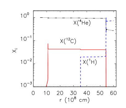
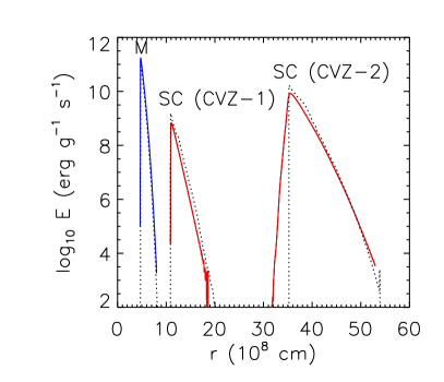
Figure 3: Left: Chemical composition of the helium core in model heflpopIII.2d.2 (SC). Right: Nuclear energy production rate as a function of radius $r$. Initial rates (at t=0) are indicated by dotted-black curves. Rates in model heflpopI.3d (SC) at $t=6400\,$s (solid-red), and in model M at $t\sim 10^{5}\,$ s (solid-blue), respectively.

Model M contains the chemical species ¹H, ³He, ⁴He, ¹²C, ¹³C, ¹⁴N, ¹⁵N, ¹⁶O ,¹⁷O,²⁴Mg, and ²⁸Si. However, since we are not interested in details of its chemical evolution, we considered only the abundances of ⁴He, ¹²C, and ¹⁶O in our hydrodynamic simulations. This is justified as the triple $\alpha$ reaction dominates the nuclear energy production rate during the core helium flash. For the remaining composition we assume that it can be represented by a gas with a mean molecular weight equal to that of ²⁰Ne, as its nucleon number agrees well with the average nucleon number of the neglected nuclear species.

The stellar model had to be relaxed into hydrostatic equilibrium after it was mapped to the numerical grid of our hydrodynamics code. This was achieved with an iterative procedure, which keeps the density distribution of the model almost constant, but modifies its pressure distribution to achieve hydrostatic equilibrium (Mocák 2009). This mapping process has a negligible effect on the stellar structure.

2.2 Initial stellar model SC

The initial model SC (Tab. 1, Fig. 1 to 3) was computed by Simon W. Campbell using the Monash/Mount Stromlo stellar evolution code (MONSTAR) (Campbell & Lattanzio 2008; Wood & Zarro 1981). It corresponds to a metal-free Pop III star with a mass of 0.85 M_⊙  near the peak of the core helium flash. Metal-free stars with masses $\gtrsim 1\leavevmode\nobreak\ \mbox{M${}_{\odot}$\,}$ do not undergo the core helium flash (as opposed to $M\lesssim 2.2\,\mbox{M${}_{\odot}$\,}$ at solar metallicity). The helium core flash commences with a very off-center ignition of helium in a relatively dense environment under degenerate conditions, and results in a fast growing convection zone powered by helium burning that relatively quickly reaches the surrounding hydrogen shell (Fujimoto et al. 1990). This causes sudden mixing of protons down into the hot helium core (Fig. 3), and leads to rapid nuclear burning via the CNO cycle i.e., a hydrogen flash. Since the core helium flash is still ongoing we refer to this as a “Dual Core Flash” (DCF). We note that this event has also been referred to as “helium flash induced mixing” (Schlattl et al. 2001; Cassisi et al. 2003; Weiss et al. 2004), and “helium flash-driven deep mixing” (Suda et al. 2004). The CNO burning leads to an increase of the temperature inside the helium-burning driven convection zone, and causes it to split into two. The result is a lower convection zone still powered by helium burning and a second one powered by the CNO cycle (Fig. 3, [right panel]). In the following we will refer to the split convection zone as a double convection zone.

The electron degeneracy in the double convection zone has already been significantly lifted to $\psi\sim-2$. It can be shown that for a degeneracy parameter $\psi<-2$, the gas pressure is essentially that of a nondegenerate gas (Clayton 1968). This confirms our previous conclusion based on the ratio of the Fermi and thermal energy of the electrons (Sect. 2).

In our hydrodynamic simulations we considered a shell from model SC which extends from $r=5\times 10^{8}\,$cm to $r=6\times 10^{9}\,$cm containing the double convection zone. Initially, the inner convection zone (powered by triple-$\alpha$ burning) covers a region from $r\approx 11\times 10^{8}\,$cm (local pressure scale height $6\times 10^{8}\,$cm) to $r\approx 35\times 10^{8}\,$cm (local pressure scale height $7\times 10^{8}\,$cm), while the outer convection zone stretches from there up to $54\times 10^{8}\,$cm (local pressure scale height $5.2\times 10^{8}\,$cm). From the bottom to the top of the double convection zone the pressure changes by $\sim 3$ orders of magnitude from $1\times 10^{20}\mbox{\ dyn$\mbox{\ cm}^{-2}$}$ erg to $1.4\times 10^{17}\mbox{\ dyn$\mbox{\ cm}^{-2}$}$. Again, we have ensured that the region of interest was located sufficiently far away from the radial grid boundaries.

Our hydrodynamic simulations were performed adopting the mass fractions of all the species used in the corresponding stellar evolutionary calculations, namely ¹H, ³He, ⁴He, ¹²C, ¹⁴N, and ¹⁶O. Since the evolutionary model did not include ¹³C and ¹³N, we determined their mass fractions assuming that the CNO cycle had been operating in equilibrium. The remaining composition is represented by a gas with the molecular weight of ²⁰Ne.

The model was relaxed to hydrostatic equilibrium in the same manner as in case of model M. This process resulted in small fluctuations in the temperature profile (Fig. 2), which were smeared out after the onset of convection.

3 Input physics

The input physics of our hydrodynamic simulations is identical to that one described in Mocák et al. (2008), except for the number of nuclear species employed in the simulations based on the initial model SC. We use an equation of state that includes contributions from radiation, ideal Boltzmann gases, and an electron-positron component (Timmes & Swesty 2000). Thermal transport was neglected as the maximum amount of energy transported by radiation and heat conduction is smaller than the convective flux by at least seven (three) orders of magnitude in model M (SC). Neutrinos act as a nuclear energy sink, but carry away less than $<10^{2}\mbox{$\mbox{\ erg }\mbox{\ g}^{-1}\mbox{\ s}^{-1}$}$. This is a negligible amount (especially for the timescales covered by our simulations) when compared to the maximum nuclear energy production $\dot{\epsilon}$, which is $\sim 10^{11}\mbox{$\mbox{\ erg }\mbox{\ g}^{-1}\mbox{\ s}^{-1}$}$ for model M, and $\sim 10^{10}\mbox{$\mbox{\ erg }\mbox{\ g}^{-1}\mbox{\ s}^{-1}$}$ in model SC, respectively (Fig.3).

3.1 Nuclear reactions

We employed two different nuclear networks for our simulations, as the nuclear species considered in models M and SC differ. The nuclear reaction network used in the hydrodynamic simulation based on the initial model M (Tab. 1) consists of four nuclei (Sect. 2.1) coupled by seven reactions. The network is identical to that one described by Mocák et al. (2008) i.e.,

He4	+	C12	$\rightarrow$	O16	+	$\gamma$
He4	+	O16	$\rightarrow$	Ne20	+	$\gamma$
O16	+	$\gamma$	$\rightarrow$	He4	+	C12
Ne20	+	$\gamma$	$\rightarrow$	He4	+	O16
C12	+	C12	$\rightarrow$	Ne20	+	He4
He4	+	He4	+	He4	$\rightarrow$	C12	+	$\gamma$
C12	+	$\gamma$	$\rightarrow$	He4	+	He4	+	He4

The nuclear reactions considered in the hydrodynamic simulations based on the initial model SC (Tab. 1) are described by a reaction network consisting of nine nuclei (Sect. 2.2) coupled by the following 16 reactions:

H1	+	He3	$\rightarrow$	He4	+	$\gamma$
He4	+	C12	$\rightarrow$	O16	+	$\gamma$
He4	+	N13	$\rightarrow$	H1	+	O16
H1	+	C13	$\rightarrow$	N14	+	$\gamma$
H1	+	C12	$\rightarrow$	N13	+	$\gamma$
H1	+	O16	$\rightarrow$	He4	+	N13
He4	+	O16	$\rightarrow$	Ne20	+	$\gamma$
C12	+	C12	$\rightarrow$	He4	+	Ne20	+	$\gamma$
N13	+	$\gamma$	$\rightarrow$	H1	+	C12
N14	+	$\gamma$	$\rightarrow$	H1	+	C13
O16	+	$\gamma$	$\rightarrow$	He4	+	C12
Ne20	+	$\gamma$	$\rightarrow$	He4	+	O16
C12	+	$\gamma$	$\rightarrow$	He4	+	He4	+	He4
He4	+	He4	+	He4	$\rightarrow$	C12	+	$\gamma$
He3	+	He3	$\rightarrow$	H1	+	H1	+	He4	+	$\gamma$
H1	+	H1	+	He4	$\rightarrow$	He3	+	He3	+	$\gamma$

This network reproduces the nuclear energy generation rate of the original stellar model very well (Fig. 3).

Note, that although the value of the temperature maximum, $T_{max}$, is higher in model SC than in model M, the energy generation rate is lower at $T_{max}$ in model SC, because the helium mass fraction $X(^{4}$He) is smaller in that model (0.956 as compared to 0.970 for model M).

4 Hydrodynamic code and computational setup

We use the hydrodynamics code Herakles (Kifonidis et al. 2003, 2006; Mocák et al. 2008, 2009) which solves the Euler equations coupled with source terms corresponding to gravity and nuclear burning. The hydrodynamic equations are integrated with the piecewise parabolic method of Colella & Woodward (1984) and a Riemann solver for real gases according to Colella & Glaz (1984). The evolution of the nuclear species is described by a set of additional continuity equations (Plewa & Müller 1999). Self-gravity is implemented according to Müller & Steimnetz (1995) and nuclear burning is treated by the semi-implicit Bader-Deuflhard scheme (Press et al. 1992).

We performed one 3D simulation based on the initial model M, which covered roughly $27\,hrs$ of stellar evolution (Tab. 2). This model (henceforth heflpopI.3d) was evolved on a computational grid consisting of a $30\mbox{${}^{\circ}$}$-wide wedge in both $\theta$ and $\phi$-direction centered at the equator. The small angular size of the grid allowed us to achieve a relatively high angular resolution ($1\mbox{${}^{\circ}$}$) with a modest number of angular zones ($N_{\phi}N_{\theta}=30$).

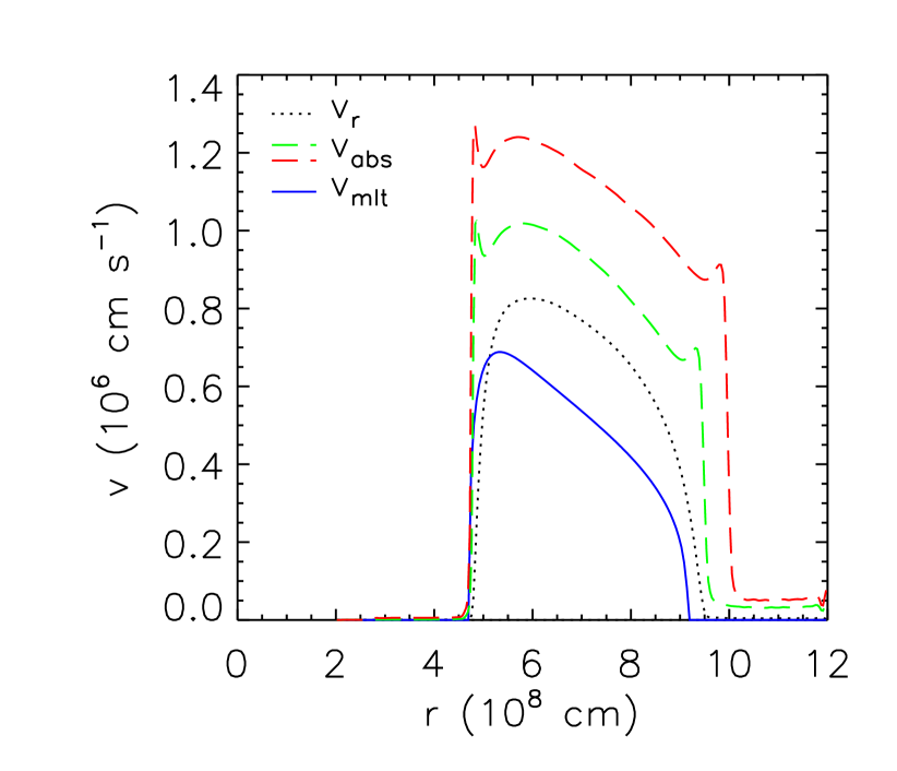
Figure 4: Radial velocity distributions for the 3D model heflpopI.3d. The dotted and green dashed lines show the time (from 10 000 s to 30 000 s) and angle-averaged radial velocity, $v_{r}$, and velocity modulus, $v_{abs}$, respectively. The red dashed line shows again the latter velocity, but time-averaged from 80 000 s to 99 000 s. The velocity predicted by the mixing-length theory ($v_{mlt}$) for the initial model M is shown by the solid blue line.

Table 2: Some properties of the 3D simulation based on model M: number of grid zones, wedge size $w$, grid resolution in $r$, $\theta$ and $\phi$ direction, estimated Reynolds number $R_{e}$ (Porter & Woodward 1994), characteristic velocity $v_{c}$ of the convective flow, typical convective turnover timescale $\tau_{cnv}$, and maximum evolutionary time $t_{max}$.

run	grid	$w$	$\Delta r$	$\Delta\theta$	$\Delta\phi$	Re	$v_{c}$	$\tau_{cnv}$	$t_{max}$
[name]	N${}_{r}\times$N${}_{\theta}\times$Nϕ	[∘]	[106 cm]	[∘]	[∘]		[10${}^{6}\,\mbox{\ cm s${}^{-1}$}$]	[s]	[s]
heflpopI.3d	$270\times 30\times 30$	30	3.7	1	1	$10^{2}$	1.1	1000	100000

In addition, we performed two 2D (henceforth models heflpopIII.2d.1 and heflpopIII.2d.2) and one 3D simulation (henceforth model heflpopIII.3d) based on the initial model SC covering about $1.8\,hrs$ and $0.39\,hrs$ of stellar evolution, respectively (Tab. 4). We used a computational grid consisting of a $50\mbox{${}^{\circ}$}$-wide angular wedge centered at the equator in case of models heflpopIII.2d.1 and heflpopIII.3d, and of a $120\mbox{${}^{\circ}$}$ wedge in case of model heflpopIII.2d.2.

We imposed reflective boundary conditions in the radial direction and transmissive ones in the angular directions in all our multi-dimensional simulations.

Figure 5: Convective and kinetic energy fluxes ($F_{C}$ and $F_{K}$, respectively) as a function of radius averaged (from 33 000 s to 53 000 s) over about 20 convective turnover timescales for the 3D model heflpopI.3d. The dotted vertical lines mark the edges of the single convection zone in the initial model M according to the Schwarzschild criterion.

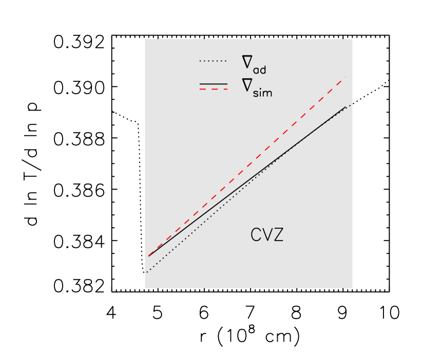
Figure 6: Radial distribution of the adiabatic temperature gradient $\nabla_{ad}$ (dotted) obtained using the EOS, and of the temperature gradient of the 3D model heflpopI.3d averaged over the first 460 s of its evolution (dashed-red), and over a period of 13000 s between 33000 s and 46000 s (solid-black), respectively. The latter gradients shown are actually linear fits to the model data. The gray shaded region marks the single convection zone CVZ.

5 Results

In this section, we first present the characteristics of the hydrodynamic simulation based on the initial model M, i.e., model heflpopI.3d, which shows a fast growth of the convection zone (Sect. 5.1). A growth rate of this magnitude likely leads to a hydrogen injection phase (Sect. 5.2), which may resemble the one seen in the initial model SC, whose hydrodynamic properties are discussed in Sect.5.3.

5.1 Single flash

Table 2 provides some characteristic parameters of our 3D simulation heflpopI.3d based on the initial model M. After convection reaches a quasi steady-state in this model, the maximum temperature rises at the rate of 80  K s^-1, i.e., only 20% slower than predicted by canonical stellar evolution theory. This corresponds to an increase of the nuclear energy production rate from $2.4\times 10^{42}\mbox{$\mbox{\ erg }\mbox{\ s}^{-1}$}$ at $t\sim 20\,000\,$s to $5.5\times 10^{42}\mbox{$\mbox{\ erg }\mbox{\ s}^{-1}$}$ at $t\sim 99\,000\,$s. Consequently, the maximum convective velocities rise by 26% from about $10^{6}\mbox{\ cm s${}^{-1}$}$ to $1.26\times 10^{6}\mbox{\ cm s${}^{-1}$}$. As illustrated in Fig. 4 these velocities match those predicted by the mixing length theory quite well. During the first third of the simulation (up to about $30\,000\,$s) the angle and time averaged radial velocity in the convective layer exceeds the velocity predicted for inital model M by the mixing-length theory, $v_{mlt}$, by about 20%, while the velocity modulus, $v_{abs}$, is about 30% larger than $v_{mlt}$. Towards the end of our simulation the angle and time averaged modulus of the velocity is about twice as large as $v_{mlt}$.

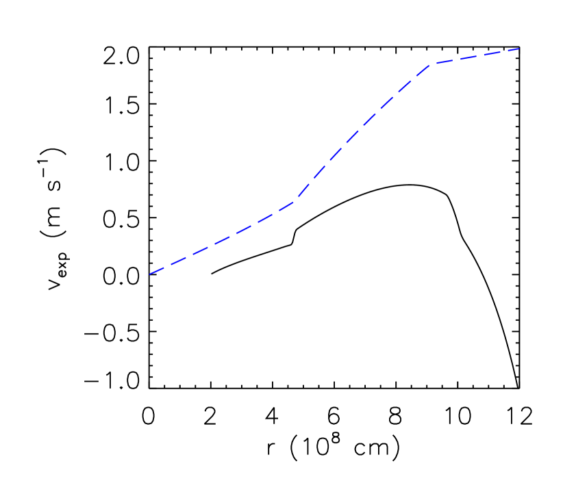
Figure 7: Radial distribution of the expansion velocity, $v_{exp}$, in the 3D model heflpop1.3d (solid) compared with the expansion velocity predicted by the stellar evolutionary calculations (dashed-blue) for the initial model M.

Contrary to our previous study (Mocák et al. 2009), we do not find a sub-adiabatic gradient in the outer part of the convection zone. . The reason for this difference is probably the increased grid resolution of our present 3D simulation, which results in less heat diffusion due to numerical dissipation, and hence a super-adiabatic temperature gradient similar to the initial one (Fig. 6)

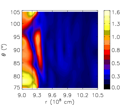
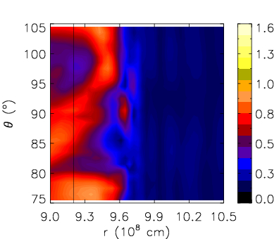
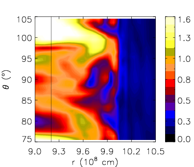
Figure 8: Color maps of the modulus of the velocity (in units of $10^{6}\mbox{\ cm s${}^{-1}$}$) near the outer boundary of the convection zone for the 3D model heflpopI.3d in the meridiononal plane $\phi=0\mbox{${}^{\circ}$}$ at three different epochs: $t_{1}=3295\,$s (left), $t_{2}=49\,385\,$s (middle), and $t_{3}=97\,655\,$s (right).

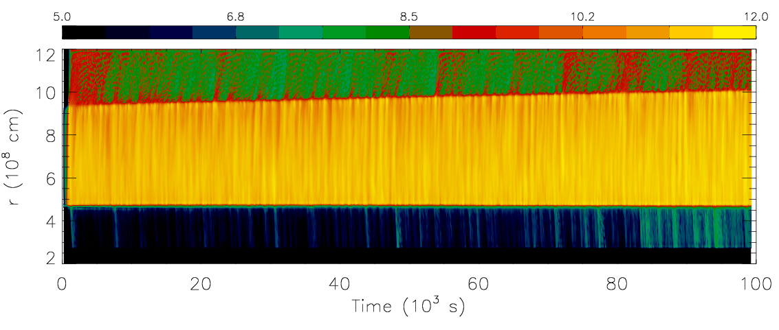
Figure 9: Temporal evolution of radial distribution of the (color coded) logarithm of the angular averaged kinetic energy density (in $\mbox{\ erg }\mbox{\ g}^{-1}$) in the 3D model heflpopI.3d. The growth of the size of the convection zone due to the turbulent entrainment, mainly at its outer boundary, is clearly visible.

At a radius $r\sim 5.5\times 10^{8}\,$cm convection transports almost 90% of the liberated nuclear energy, i.e., $2.1\times 10^{42}\mbox{$\mbox{\ erg }\mbox{\ s}^{-1}$}$ (Fig. 5). The energy flux due to thermal transport is negligible (Sect. 3).

We observe internal gravity waves or g-modes in the convectively stable layers. These g-modes are strongly instigated only during certain evolutionary phases (g-mode events) because of the intermittent nature of the convective flow. The g-mode events are correlated with outbursts in kinetic energy of the convection zone (Meakin & Arnett 2007). It appears that the frequency of g-mode events increases as the flow gains strength (Fig. 9).

Figure 10: Angular averaged ¹²C mass fraction as a function of radius near the inner (left) and outer edge (right) of the convection zone in the 3D model heflpopI.3d at $t=100\,000\,$s. The thick line gives the corresponding temperature stratification, and the vertical dotted lines mark the edges of the convection zone at $t=0\,$s. The observed entrainment velocities v_e are given in both panels, too.

We observe a growth of the size of the single convection zone due to turbulent entrainment at the convective boundary on a dynamic timescale (Figs. 8 to 10), and estimate the corresponding entrainment speeds by adopting the prescription of Meakin & Arnett (2007). Turbulent entrainment involves mass entrainment (Fig. 8) rather than a diffusion process, which acts to reduce the buoyancy jump at the convective boundary allowing matter to be mixed further. The entrainment velocity or the interface migration velocity, $u_{e}$, is given by (see Eq. (32) of Meakin & Arnett (2007)

$$u_{e}=\frac{\Delta q}{hN^{2}},$$ (6)

where $\Delta q$ is the buoyancy jump, i.e., the variation of the buoyancy flux $q$ across the convective boundary of thickness $h$, and $N^{2}$ the square of the Brunt-Väisälä buoyancy frequency. The buoyancy flux is defined as $q=g\rho^{\prime}v^{\prime}/\rho$, where $g,\rho$, and $v$ are the gravitational acceleration, the density, and the velocity, respectively. The quantities $\rho^{\prime}$ and $v^{\prime}$ denote fluctuations around the corresponding mean quantities $\rho_{0}$ and $v_{0}$, i.e., $\rho=\rho_{0}+\rho^{\prime}$ and $v=v_{0}+v^{\prime}$, respectively. The thickness $h$ of the convective boundary is defined as the half width of the peak in the mass fraction gradient of ¹²C, which varies rapidly at the boundary. The entrainment velocities (averaged over 20 convective turnovers at the end of the simulation) obtained by this formula are summarized in Tab. 3 together with those derived from measuring the position of the convective boundary in our hydrodynamic simulations.

Table 3: Some quantities characterizing the convective boundaries of the 3D model heflpopI.3d : buoyancy jump $\Delta q$ (in $\mbox{\ erg }\mbox{\ g}^{-1}\mbox{\ s}^{-1}$), square of the Brunt-Väisälä buoyancy frequency $N^{2}$, interface migration velocity calculated according to Eq. 6, $u_{e}$, and obtained from our simulation, $v_{e}$, and expansion velocity $v_{exp}$, at the inner and outer convective interface of thickness $h$, respectively.

pos	$\Delta q$	$h$	$N^{2}$	$u_{e}$	$v_{e}$	$v_{exp}$
	[$10^{8}$]	[$10^{7}$cm]	[ rad${}^{2}\mbox{\ s}^{-2}$ ]	[ m s-1]	[ m s-1]	[ m s-1]
inner	9.7	1.0	0.92	1.1	$<$0.6	0.4
outer	6.5	1.2	0.14	3.9	6.7	0.8

The entrainment velocity derived for our models, $v_{e}$, are calculated by measuring the radial position of the convective boundaries defined by the condition X(¹²C) $=2\times 10^{-3}$, as ¹²C is much less abundant outside the convection zone (Fig. 10). The expansion velocity (zero in hydrostatic equilibrium) is given by $v_{exp}=\dot{m}_{r}/4\pi r^{2}\rho$, where $\dot{m}_{r}$ is the partial time derivative of the mass $m_{r}$ of a shell of density $\rho$ at a radius $r$.

We find in our models that $v_{e}$, which includes the expansion velocity $v_{exp}$, agrees very well with the velocity $u_{e}$ predicted by theoretical considerations of the entrainment process (see Eq. 6), despite the crude estimate of the divergence of the buoyancy flux through $\Delta q/h$. The velocity given by the difference $v_{e}-v_{exp}$, which is the actual entrainment speed in our models, differs from the theoretically estimate $u_{e}$ by 0.9 m s^-1 and 2.0 m s^-1 at the inner and outer convection boundary, respectively.

It seems that turbulent entrainment is a robust process which has been seen to operate under various conditions in different stars (Mocák et al. 2009; Meakin & Arnett 2007). This process may be behind the observed Al/Mg anti-correlation (Shetrone 1996a, b; Yong et al. 2006), which could result from an injection of hydrogen into the helium core and a subsequent dredge-up (Langer et al. 1993; Langer & Hoffman 1995; Langer et al. 1997; Fujimoto et al. 1999).

Table 4: Some properties of the 2D and 3D hydrodynamic models based on initial model SC: wedge size $w$, number of grid points in $r$, $\theta$, and $\phi$ direction, estimated Reynolds numbers $R_{e1}$, $R_{e2}$ (Porter & Woodward 1994), characteristic flow velocities, $v_{c1}$ and $v_{c2}$, and typical convective turnover timescales, $\tau_{cnv1}$ and $\tau_{cnv2}$, for the bottom and top part of the convection zone, respectively. $t_{max}$ is the maximum evolutionary time.

run	grid	$w$	$\Delta r$	$\Delta\theta$	$\Delta\phi$	$R_{e1}$	$R_{e2}$	$v_{c1}$	$v_{c2}$	$\tau_{cnv1}$	$\tau_{cnv2}$	$t_{max}$
[name]	N${}_{r}\times$N${}_{\theta}\times$Nϕ	[∘]	[$10^{6}$ cm]	[∘]	[∘]			[$10^{6}\,\mbox{\ cm s${}^{-1}$}$]	[$10^{6}\,\mbox{\ cm s${}^{-1}$}$]	[ s ]	[ s ]	[ s ]
heflpopIII.2d.1	$720\times 50$	50	7.6	1	-	$10^{3}$	$10^{2}$	1.3	1.0	2900	2400	1400
heflpopIII.2d.2	$1500\times 120$	120	3.7	1	-	$10^{5}$	$10^{3}$	1.7	1.0	2200	2400	6400
heflpopIII.3d	$720\times 50\times 50$	50	7.6	1	1	$10^{2}$	$10^{2}$	0.4	0.3	9500	8000	1400

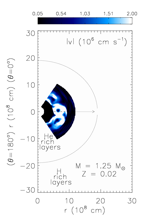
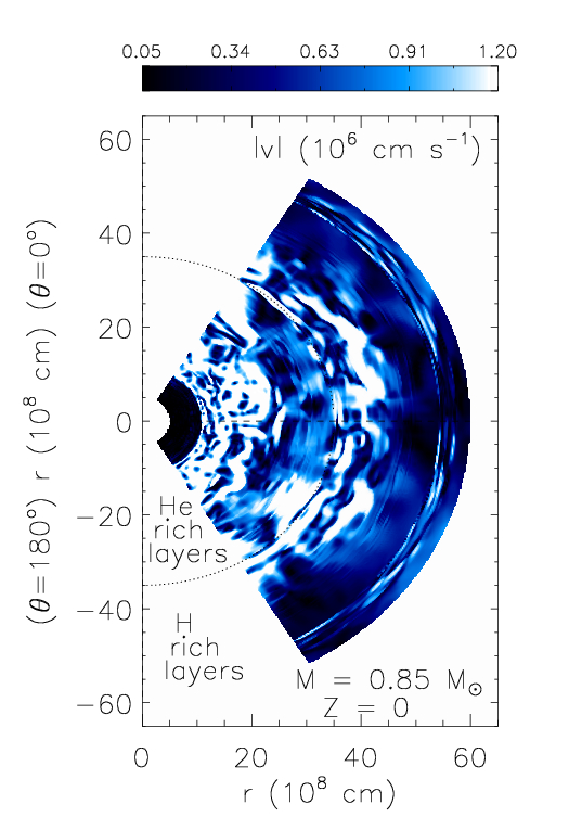
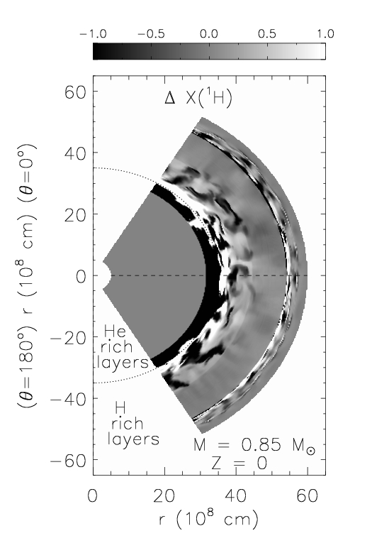
Figure 11: Snapshots of the spatial distribution of the velocity modulus $|\mbox{v}|$ (in units of $10^{6}\mbox{\ cm s${}^{-1}$}$) of a typical 2D hydrodynamic model with a single convection zone (left), and for the 2D hydrodynamic model heflpopIII.2d.2 at 1250 s (middle). The right hand panel shows the double convection zone highlighted by using the hydrogen contrast $\Delta X(^{1}\mbox{H})=\mbox{100}\times(X(^{1}\mbox{H})-\langle X(^{1}\mbox{H})\rangle_{\theta})/\langle X(^{1}\mbox{H})\rangle_{\theta}$ at the same time, where $\langle\rangle_{\theta}$ denotes a horizontal average at a given radius. The arrow indicates the growth of the single convection zone, while the dotted line represents the border between the helium and hydrogen rich layers.

5.2 From the single to the dual flash

If the radial position of the innermost edge of the hydrogen-rich layers was fixed at its initial value in model M at $r=1.9\times 10^{9}\,$cm (no expansion), the outer convection boundary would reach the hydrogen-rich layer due to the turbulent entrainment within only 17 days, and the helium core would experience a dual core flash (DCF) known from low-mass Pop III stars.

However, the hydrogen layer will initially expand outwards at a faster rate than the outer convective boundary (Fig. 7). This delays the expected onset of the hydrogen injection a little, as the outer convection boundary has to catch up with the hydrogen layer expanding away from the HeCZ. As the expansion velocities of our hydrodynamic models are biased by the imposed reflective boundaries in radial direction, we did not use these values here. To get an estimate for the onset of the hydrogen injection we instead used the expansion speed of the helium core as predicted by stellar evolutionary calculations (Tab. 3), and find that the injection of hydrogen into the helium core should take place within 23 days.

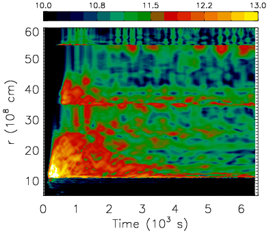
Figure 12: Temporal evolution of the radial distribution of the (color coded) logarithm of the angular averaged radial ($v_{r}^{2}/2$; upper panel) and angular $v_{\theta}^{2}/2$; lower panel) component of the specific kinetic energy (in $\mbox{\ erg }\mbox{\ g}^{-1}$) of the 2D model heflpopIII.2d.2.

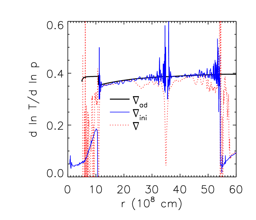
Figure 13: Adiabatic temperature gradient $\nabla_{ad}$ (solid-black), temperature gradient of the 2D model heflpopIII.2d.2 averaged from 1000 s to 3200 s (dashed-red), and temperature gradient of the initial model SC (solid-blue), respectively, as a function of radius.

This is still a very short time, and even if our estimate for the time until the onset of the hydrogen injection was wrong by 5 orders of magnitude, the injection will occur before the first subsequent mini helium flash takes place, which is supposed to occur in roughly $10^{5}$ years.

Figure 11 shows snapshots from 2D hydrodynamic simulations (Mocák et al. 2009) of a (single) core helium flash based on initial model M (left panel), and of a dual core (helium + hydrogen) flash based on initial model SC (middle and right panels). The figure suggests that that even if the core helium flash starts out with a single convection zone in a low-mass Pop I star, this convection zone may evolve due to its growth by turbulent entrainment (indicated by the arrow in the left panel of the figure) into a double convection zone like that found in models of Pop III stars. Although the upper boundary of the single convection zone is still far away from the hydrogen-rich layers at the end of the simulation, it should get there eventually. We find no reason in any of our 2D or 3D simulations including the new model heflpopI.3d why turbulent entrainment should cease before the outer convective boundary reaches the edge of the helium core. Actually, as the maximum temperature of the helium core grows and the convective flow becomes faster, entrainment will eventually speed up (Mocák et al. 2009).

On the other hand, subsequent mini helium flashes are unlikely to occur, because we estimate that at the observed entrainment velocity the inner convective boundary will reach the center of the star in $\gtrsim$ 90 days. Note in this respect that the fast entrainment speed of the inner convective boundary derived from our previous 2D models (Mocák et al. 2008) is not confirmed by the new 3D model. The entrainment rate is actually slower in the new 3D model, which was expected (Mocák et al. 2009).

The turbulent entrainment at the inner convection boundary heats the layers beneath at a rate $\delta T/\delta t\sim 630$ K s^-1, i.e., it is quite efficient in lifting the electron degenaracy in the matter below the convection zone.

According to the above discussion we propose a somewhat speculative scenario for the core helium flash in low-mass Pop I stars. These stars ignite helium burning under degenerate conditions and develop a single convection zone, which at some point extends due to turbulent enrainment up to their hydrogen-rich surface layers. The convection zone eventually penetrates these layers, and dredges down hydrogen into the helium core. This ignites a secondary flash driven by CNO burning, which together with triple-$\alpha$ burning and inwards turbulent entrainment leads eventually to the lifting of the core’s degeneracy, i.e., the star will settle down on the horizontal branch.

5.3 Dual flash

We have performed three simulations of the core helium flash based on the Pop III initial model SC which possesses two convection zones sustained by helium and CNO burning, respectively. Some characteristic properties of these dual flash simulations are summarized in Table 4.

5.3.1 Model heflpopIII.2d.2

Despite a nuclear energy production rate due to CNO burning in the outer convection zone ($\dot{\epsilon}_{max}\sim 1.4\times 10^{10}\mbox{$\mbox{\ erg }\mbox{\ g}^{-1}\mbox{\ s}^{-1}$}$, which is roughly eight times higher than that due to triple-$\alpha$ burning in the inner zone $\dot{\epsilon}_{max}\sim 1.7\times 10^{9}\mbox{$\mbox{\ erg }\mbox{\ g}^{-1}\mbox{\ s}^{-1}$}$), convective motions first appear within the inner convection zone after about 200 s. The onset of convection in the outer zone is delayed until about 500 s (Fig. 12, Fig. 16). After some time the model relaxes into a quasi steady-state, where the r.m.s values of the angular velocity are comparable or even larger than those of the radial component (Fig. 12). This property of the velocity field implies the presence of g-modes or internal gravity waves (Asida & Arnett 2000), which is a surprising fact. G-modes should not exist in the convection zone according to the canonical theory, as any density perturbation in a convectively unstable zone will depart its place of origin exponentially fast (Kippenhahn & Weigert 1990) until the flow becomes convectively stable.

When convection begins to operate in both zones, the total energy production rate temporarily drops by $\sim$ 20%, but continues to rise at a rate of $2.8\times 10^{36}$$\mbox{\ erg }\mbox{\ s}^{-2}$  after $t\approx 2000\,$s. Nevertheless, the convective flow decays fast in both convection zones – at a rate of $4\times 10^{40}$$\mbox{\ erg }\mbox{\ s}^{-1}$(Fig. 16), probably because the initial conditions represented by the stabilized initial model are too different from those of the original stellar model. They disfavor convection since the stabilized model has a slightly lower temperature gradient than the original one (Fig. 2, Fig. 13). However, we note that stabilization of the initial model was essential to prevent it from strongly deviating from hydrostatic equilibrium.

Shortly after convection is triggered in both the outer and the inner zone this double convection structure vanishes, and after about 2000 s there is no evidence left for two separate convection zones (Fig. 12).

Due to the relatively short temporal coverage of the evolution and due to the decaying convective flow, we did not analyze the energy fluxes and turbulent entrainment of this model. Penetrating plumes do not exist in the convection zone (initially determined by the Schwarzschild criterion), as it is dominated rather by g-modes. Hence, firm conclusions are difficult to derive, but we plan to address this issue elsewhere. We are now going to introduce some basic characteristic of internal gravity waves or g-modes that are required to draw further conclusions.

G-modes

In a convectively stable region, any displaced mass element or blob (density perturbation) is pushed back by the buoyancy force. On its way back to its original position, the blob gains momentum and therefore starts to oscillate around its original position. Assuming, the element is displaced by a distance $\Delta r$, has an excess density $\Delta\rho$, and is in pressure equilibrium with the surrounding gas ($\Delta$P = 0), one can derive an equation for the acceleration of the element:

$$\frac{\partial^{2}(\Delta r)}{\partial t^{2}}=\frac{g\delta}{H_{p}}\left[\nabla_{\mbox{ele}}-\nabla_{\mbox{surr}}+\frac{\varphi}{\delta}\nabla_{\mu}\right]\Delta r$$ (7)

where $g$ is the gravitational acceleration, $H_{p}=|p/\partial_{r}p|$ is the pressure scale height, $\nabla\equiv d\ln T/d\ln P$, $\nabla_{\mu}\equiv d\ln\mu/d\ln P$, $\delta\equiv\partial\ln\rho/\partial\ln T$, and $\varphi\equiv\partial\ln\rho/\partial\ln\mu$.

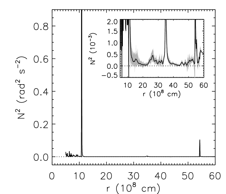
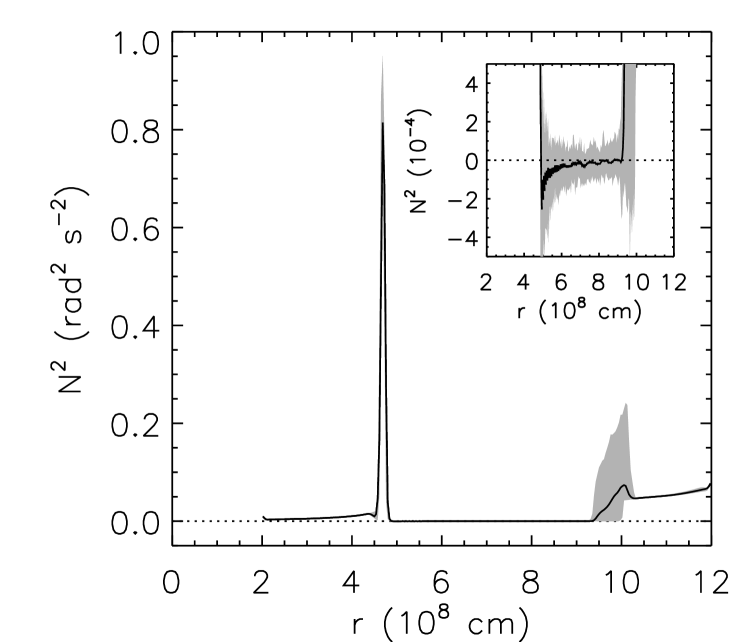
Figure 14: Radial distributions of the (square of the) Brunt-Väisälä buoyancy frequency $N^{2}$ in the 2D model heflpopIII.2d.2 averaged between 1480 s and 6000 s (top), and in the 3D model heflpop1.3d averaged between 6600 s and 100 000  (bottom), respectively. The angular and temporal variation of $N^{2}$ at a given radius are indicated by the gray shaded region. The inserts show a zoom of the region around $N^{2}=0$ to enlarge the variations of $N^{2}$ in the convection zone which are $\hbox{\raise 2.15277pt\hbox{$<$} \kern-11.00008pt\lower 2.15277pt\hbox{$\sim$}}10^{-3}$.

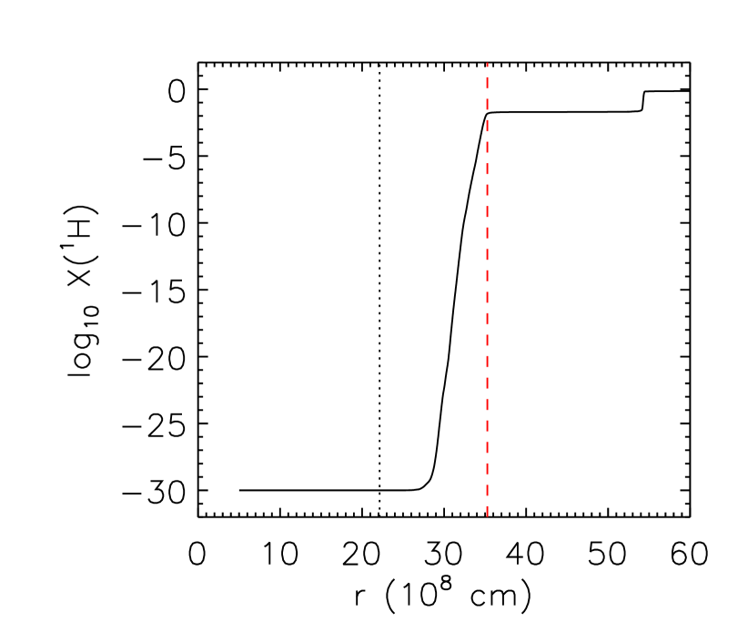
Figure 15: Hydrogen mass fraction as a function of radius for the 2D model heflpopIII.2d.2 at $t=6405\,$s. The vertical lines mark the initial border between hydrogen and helium rich layers (dashed-red), and the layer (dotted) where the timescale for proton capture on ¹²C equals 10${}^{2}\,$s ($T\sim 1\times 10^{8}\,$K).

Let us assume now that the element, after an initial displacement $\Delta r_{0}$, moves adiabatically ($\nabla_{\mbox{ele}}=\nabla_{\mbox{ad}}$) through a convectively stable layer. The element is accelerated back towards its equilibrium position and starts to oscillate around this position according to the solution of Eq. (7):

$$\Delta r=\Delta r_{0}\leavevmode\nobreak\ e^{i\leavevmode\nobreak\ N\leavevmode\nobreak\ t}\,,$$ (8)

where the (square of the) Brunt-Väisälä frequency is given by

$$N^{2}=\frac{g\delta}{H_{P}}\left(\nabla_{\mbox{ad}}-\nabla_{\mbox{surr}}+\frac{\varphi}{\delta}\nabla_{\mu}\right)$$ (9)

In a convectively unstable region (assuming $\nabla_{\mu}=0$), Eq.(9) implies $N^{2}<0$, i.e., $N$ is imaginary. Thus, the displaced element moves exponentially away from its initial position, instead of oscillating around it, as it is the case for g-modes or internal gravity waves and $N^{2}>0$.

G-modes appear in layers of gas stratified under gravity and are spatial oscillatory displacements of density perturbations. The dispersion relation of such density displacements, assumed to vary as $\exp[i({\bf{k}}\cdot{\bf{r}}-\omega t)]$, reads (Dalsgaard 2003)

$$\omega^{2}=\frac{N^{2}}{1+k^{2}_{r}/k^{2}_{h}}\,,$$ (10)

where $\omega$ is the temporal frequency of the density displacements, and k_r and k_h are the radial and horizontal components of the wave number k, respectively. The dispersion relation tells us that any density perturbation must (under influence of buoyancy forces) displace matter horizontally to propagate vertically. This will give rise to matter motion resembling horizontal fingers as $\omega$ approaches the Brunt-Väisälä frequency for large k_h ($k^{2}_{r}/k^{2}_{h}\rightarrow 0$ and $\omega^{2}\rightarrow N^{2}$).

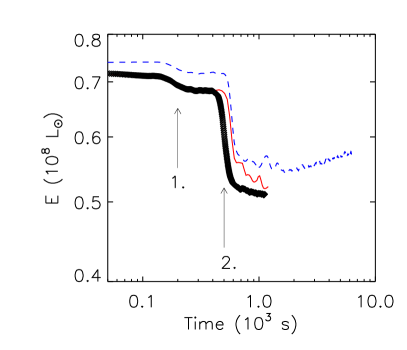
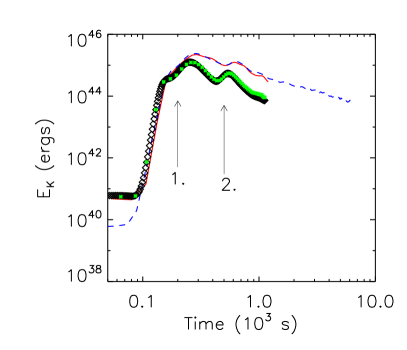
Figure 16: Left panel: Temporal evolution of the nuclear energy production rate $E$ (left) in units of the solar luminosity $L_{\odot}$ and the kinetic energy $E_{K}$ (right) for the models heflpopIII.3d (diamonds-black), heflpopIII.2d.1 (solid-red), and heflpopIII.2d.2 (dashed-blue), respectively. The green stars give the behavior of a 3D model with the same properties as model heflpopIII.3d, but with nuclear burning switched off. The vertical arrows, labeled 1. and 2., mark the onset of convection in the lower and upper convection zone of the double convection structure, respectively.

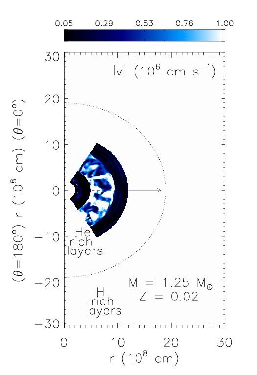
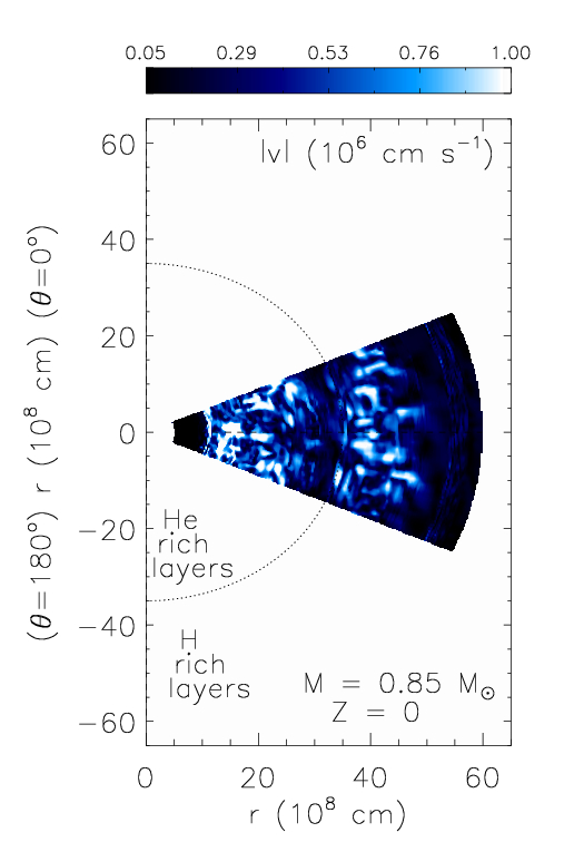
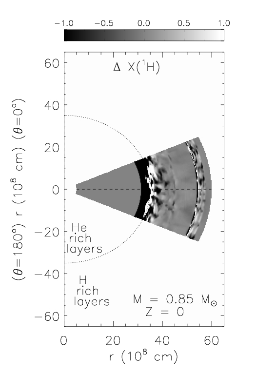
Figure 17: Snapshots of the spatial distribution of the velocity modulus $|\mbox{v}|$ (in units of $10^{6}\mbox{\ cm s${}^{-1}$}$) for a typical 3D hydrodynamic model with a single convection zone (left), and for model heflpopIII.3d at $t=1300\,$s with its double convection zone (middle) in the meridional plane $\phi=0\mbox{${}^{\circ}$}$. The right panel shows the hydrogen convection zone highlighted by using the hydrogen contrast $\Delta X(^{1}\mbox{H})=\mbox{100}\times(X(^{1}\mbox{H})-\langle X(^{1}\mbox{H})\rangle_{\theta})/\langle X(^{1}\mbox{H})\rangle_{\theta}$, where $\langle\rangle_{\theta}$ denotes a horizontal average at a given radius. The arrow indicates the growth of the single convection zone, while the dotted line represents the border between the helium and hydrogen rich layers .

We find such horizontal structures in our models (Fig. 11) visible mainly in the radiative layer of the splitted convection zone (Fig. 11). By decomposition of the specific kinetic energy density of the model into the radial (v${}_{r}^{2}$/2) and horizontal (v${}_{\theta}^{2}$/2) component, we also find that the horizontal displacements are characterized by higher values of the kinetic energy density compared to the corresponding values of the vertical displacements already 2000 s after the start of the simulation (Fig. 12). Additionally, $N^{2}$ is mostly positive in these models (Fig. 14), indicating convective stability throughout the double convection zone. This proves the existence of internal gravity waves in the decaying double convection zone. The situation is different in our 3D model heflpop1.3d, where $N^{2}$ is (on average) small and negative everywhere in the single convection zone (Fig. 14).

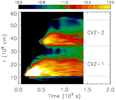
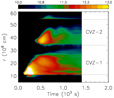
Figure 18: Temporal evolution of the radial distribution of the (color coded) logarithm of the angular averaged kinetic energy density (in $\mbox{\ erg }\mbox{\ g}^{-1}$) of models heflpopIII.2d.1 (left) and heflpopIII.3d (right), respectively. The horizontal dotted lines mark the boundaries of the double convection zone one part being sustained by the helium burning (CVZ-1) and the other one by the CNO cycle (CVZ-2).

Within the double convection zone originally determined by the Schwarzschild criterion the temperature gradient drops everywhere below the adiabatic one (Fig. 13). It does not imply that convection must cease. Even if the temperature gradient is not everywhere super-adiabatic nuclear burning may create hot blobs, which although cooling faster than the environment can still be hotter than the latter, and thus can rise upwards.

This supports our conclusions based on the distribution of the Brunt-Väisälä frequency, which might be, however, a result of insufficient resolution, as the gradient increases with increasing resolution. Consequently, we do not find the typical 2D convective pattern characterized by vortices in the double convection zone at later times t$\leavevmode\nobreak\ >2000\leavevmode\nobreak\ s$.

Radiative barrier

Stellar evolutionary calculations of low-mass Pop III stars predict that the helium flash-driven convection zone splits into two, when the hydrogen-burning luminosity (driven by the entrainment of H) exceeds the helium-burning luminosity. At this point, a radiative barrier is created between both convective zones, as energy flows inwards from the layers where hydrogen-burning takes place. The radiative barrier is thought to prevent the flow of isotopes into the helium burning layers and vice versa, hence preventing the reaction ¹³C ($\alpha$, n) ¹⁶O to become a source of neutrons. Also an eventual mixing of isotopes from the helium-burning layer into the stellar atmosphere should be inhibited. However, this scenario is difficult to prove due to numerical problems arising when modeling this event in 1D (Hollowell et al. 1990).

Our hydrodynamic model heflpopIII.2d.2 with the double convective zone shows that the radiative barrier allows for some interaction between both zones via g-modes (Fig. 11, Fig. 12). In addition, there is some mixing of hydrogen into the radiative layer, which was initially completely devoid of hydrogen (i.e., X(¹H) = 10^-30). Hydrogen must have been mixed there either by convective motion from the hydrogen-rich layers or dredged down by penetrating convective plumes from the lower convection zone. The downward mixing of hydrogen extends to a radius of $\sim 2.84\times 10^{9}\,$cm (X(¹H) $\sim 10^{-29}$) by the end of our simulation heflpopIII.2d.2 (Fig. 15). It is likely that deeper mixing of hydrogen into the helium burning layers is not possible, since protons are captured via the reaction ¹²C (p, $\gamma$) ¹³N on timescales shorter than that on which protons are mixed inwards (Hollowell et al. 1990). At a temperature $T\sim 10^{8}\,$K ($r\sim 2.21\times 10^{9}\,$cm) the proton lifetime against capture by ¹²C is as short as $\sim 10^{2}\,$s (Caughlan & Fowler 1988). This is an order of magnitude smaller than the observed initial convective turnover timescales (Tab. 4).

5.3.2 Simulation heflpopIII.2d.1 and heflpopIII.3d

We now discuss the qualitative behavior of 2D and 3D Pop III models which were simulated using the same number of radial and angular zones, but which have a lower radial and angular resolution than the 2D model heflpopIII.2d.2 discussed in the previous subsection. The quantitative properties of the convection zone of these models will obviously be different as an increased grid resolution implies less numerical viscosity and larger Reynolds numbers. We again stress here that the characteristic Reynolds numbers in our 2D and 3D simulations (Tab. 4) are still many orders of magnitude smaller than the values predicted by theory (see Sect. 2).

The comparison between the 2D and 3D simulations, heflpopIII.2d.1 and heflpopIII.3d, provides important information on the impact of the symmetry restriction imposed in the 2D models. Contrary to the 2D models, our 3D hydrodynamic simulations of turbulent flow performed with the PPM scheme (Sect. 4) are geometrically unconstrained, i.e., in the inertial regime turbulent eddies can decay along the Kolmogorov cascade down to the finest resolved scales (Sitine et al. 2000).

Due to the large computational cost we evolved the 3D model heflpopIII.3d and the corresponding 2D model heflpopIII.2d.1 for $0.39\,$hrs of stellar life, only. We find the following qualitative differences between the 3D and 2D model (Fig. 16): (i) in 3D convection starts earlier in the outer part of the double convection zone, (ii) convective velocities are smaller there, and (iii) the convective structures have a plume-like shape in 3D (Fig. 17) and are vortex-like in 2D (Fig. 11). On the other hand, the models also exhibit the following common qualitative evolutionary properties (Fig. 16): (i) a decrease of the total nuclear energy production rate, (ii) a decrease of the maximum temperature, (iii) a decay of the velocity field in the convection zones (Fig. 18), and (iv) the presence of internal gravity waves in the radiative barrier.

The differences observed between the 2D and 3D simulation do not come at a surprise, as it is well known that 2D simulations lead to an overestimate of the flow velocities (Muthsam et al. 1995; Meakin & Arnett 2006). On the other hand, the common properties of the 2D and 3D model are also shared by the high resolution simulation heflpopIII.2d.2, except for the nuclear energy production rate, which does not decrease after convection is fully established. This implies that both our 2D model heflpopIII.2d.1 and 3D model heflpopIII.3d are not sufficiently well resolved, although they show the most important characteristics of the high resolution model heflpopIII.2d.2 described in Sect. 5.3.1, i.e., the presence of a decaying convective flow in both convection zones which are later dominated by internal gravity waves. This also holds for the intermediate radiative layer.

Contrary to the low resolution 2D model heflpopIII.2d.1, the convective velocities found for the 3D model heflpopIII.3d in the inner convection zone sustained by helium burning match those predicted by stellar evolutionary calculations relatively well, although the modulus of the velocity is about a factor of two larger. In the outer part of the convection zone, sustained by the CNO cycle, the modulus of the velocity and the individual velocity components are smaller by more than a factor of two.

Interestingly, we find convection to be triggered spontaneously in these simulations – even without nuclear burning. This is highlighted by the fact that the temporal evolution of the kinetic energy of the 3D model heflpopIII.3d with no nuclear nuclear energy production is almost identical to that of the corresponding model with burning switched on (Fig. 16). Thus, we conclude that the hydrodynamic convective flow observed in our models is mainly driven by the adopted temperature gradient which is inherited from the 1D stellar model, and is only partially sustained by nuclear burning within the hydrodynamic simulation.

6 Summary

We have performed and analyzed a 3D hydrodynamic simulation of a core helium flash near its peak in a Pop I star possessing a single convection zone (single flash) sustained by helium burning. The simulation covers 27 hrs of stellar life, or roughly 100 convective turnover timescales. In addition, we performed and analyzed 2D and 3D simulations of the core helium flash near its peak in a Pop III star which has a double convection zone (dual flash) sustained by helium and CNO burning, respectively. These simulations cover only 1.8 hrs and 0.39 hrs of stellar life, respectively, as convection dies out shortly after it appears.

The convective velocities in our hydrodynamic simulation of the single flash model and those predicted by stellar evolutionary calculations agree approximately. Contrary to our previous findings, the temperature gradient in the convection zone remains superadiabatic, probably because of the increased spatial resolution of these simulations as compared to our old models. As expected, the simulation shows that the convection zone grows on a dynamic timescale due to turbulent entrainment. This growth can lead to hydrogen injection into the helium core as predicted by stellar evolutionary calculation of extremely metal-poor or metal-free Pop III stars. Hydrogen injection leads to a split of the single convection zone into two parts separated by a supposedly impenetrable radiative zone. Our hydrodynamic simulations of the double convection zone show that the two zones vanish as their convective motion decays very fast. However, this result may be caused by an insufficient spatial grid resolution or probably because the conditions represented by the stabilized initial model are a bit different from those of the original stellar model. While the convective velocities in our 2D hydrodynamic models do not match those predicted by stellar evolutionary calculations for the double convection zone at all, a rough agreement is found in our 3D model for the velocities in the inner convection zone sustained by helium burning.