Numerical simulation study of the dynamical behavior of the Niedermayer algorithm

Abstract

We calculate the dynamic critical exponent for the Niedermayer algorithm applied to the two-dimensional Ising and $XY$ models, for various values of the free parameter $E_{0}$. For $E_{0}=-1$ we regain the Metropolis algorithm and for $E_{0}=1$ we regain the Wolff algorithm. For $-1<E_{0}<1$, we show that the mean size of the clusters of (possibly) turned spins initially grows with the linear size of the lattice, $L$, but eventually saturates at a given lattice size $\widetilde{L}$, which depends on $E_{0}$. For $L>\widetilde{L}$, the Niedermayer algorithm is equivalent to the Metropolis one, i.e, they have the same dynamic exponent. For $E_{0}>1$, the autocorrelation time is always greater than for $E_{0}=1$ (Wolff) and, more important, it also grows faster than a power of $L$. Therefore, we show that the best choice of cluster algorithm is the Wolff one, when compared to the Nierdermayer generalization. We also obtain the dynamic behavior of the Wolff algorithm: although not conclusive, we propose a scaling law for the dependence of the autocorrelation time on $L$.

Numerical methods; dynamic behavior; Cluster algorithms; XY model

1 Introduction

Numerical simulations have been widely used in the study of physical systems, specially in the last decades. The field of statistical mechanics, among others, has benefited a great deal from the use of this technique. In particular, Monte Carlo methods allowed for a precise determination of thermodynamic parameters in a variety of models, both classical and quantum. Excellent reviews on these methods can be found in Refs. [1] and [2].

In recent years, this field has seen a fast development of new algorithms, which aim to make the simulation more efficient, both in time and in memory, as well as broadening its application to more complex systems. As examples of these developments, we can recall: the calculation of the density of states through flat histograms, which allows obtaining information at any temperature from one single simulation, independent of temperature [3]; the use of bitwise operations and storage, which increases by a great deal the speed of the update process and saves memory (with the drawback that this procedure can be used only with specific models) [4]; and the introduction of cluster algorithms, which updates collections of spins, decreasing the autocorrelation time and almost eliminating critical slowing down [1, 2, 5, 6].

In this work we will focus on this last issue. In fact, critical slowing down is a serious drawback, which makes simulation of systems at, or near, critical points very inefficient. This phenomenon is measured through the scaling of the autocorrelation time, $\tau$, with the linear size of the lattice, $L$, assumed to be in the form $\tau\sim L^{z}$, for points at the critical region. The popular Metropolis algorithm, for example, when applied to the Ising model in two dimensions, presents $z\sim 2.17$ [7]. Algorithms which update clusters of spins (the so-called cluster algorithms) have a much lower value of $z$: this is the case for the Swendsen-Wang [5] and Wolff [6] algorithms, for which $z$ is approximately zero for the two-dimensional Ising model [8, 9].

An alternative (and generalization) to these last two cluster algorithms, the Niedermayer algorithm, was introduced some time ago [10] but, to the best of our knowledge, has never had his dynamic behavior studied in detail. In this work, we calculate the dynamic exponent for this algorithm, applied to the Ising and $XY$ models, for some values of the free parameter $E_{0}$ (see below), in order to determine the best choice of this parameter.

This work is organized as follows: in the next section we present the Niedermayer algorithm and relate it to Metropolis’ and Wolff’s. In Section 3 we review some features connected to the autocorrelation time and the dynamic exponent $z$, in Section 4 we present and discuss our results, and in the last section we summarize the results.

2 The Niedermayer algorithm

The Niedermayer algorithm was introduced some time ago and is an option to Wolff or Swendsen-Wang cluster algorithms. The idea is to build clusters of spins and accept their updating as a single entity, hopefully in a more efficient way, when compared to these last two algorithms. In this work, we have chosen to build the clusters according to the Wolff criterion (they can be constructed according to the Swendsen-Wang rule but the results will not differ qualitatively in two dimensions and in higher dimensions Wolff algorithm in superior to Swendsen-Wang’s). It works as follows, for the Ising model (the generalization of this algorithm for the $XY$ model is presented in the Appendix): a spin in the lattice is randomly chosen, being the first spin of the cluster. This spin is called the seed. First-neighbours of this spin may be considered part of the cluster, with a probability

$$P_{add}(E_{ij})=\left\{\begin{array}[]{ll}1-e^{K\left(E_{ij}-E_{0}\right)},&\mbox{if}\;\;E_{ij}<E_{0},\\ 0,&\mbox{otherwise},\end{array}\right.$$ (1)

where $K=J/kT$, $T$ is the temperature, $J$ is the exchange constant, and $E_{ij}$ is the energy between nearest-neighbour spins in unities of $J$ (i.e, $E_{ij}=-s_{i}s_{j}$; $s_{i},s_{j}=\pm 1$). The free parameter $E_{0}$ controls the size of the clusters and the acceptance ratio of their updating, as seen below. First-neighbours of added spins may be added to the cluster, according to the probability given above. Each spin has more than one chance to be part of the cluster, since it may have more than one first-neighbour in it. When no more spins can be added, all spins in the cluster are flipped with an acceptance ratio $A$. Assuming that, at the frontier of the cluster there are $m$ bonds linking parallel spins and $n$ bonds linking anti-parallel spins, $A$ satisfies:

$$\frac{A(a\rightarrow b)}{A(b\rightarrow a)}=\left[e^{2K}\left(\frac{1-P_{add}(-J)}{1-P_{add}(J)}\right)\right]^{n-m},$$ (2)

where $a\rightarrow b$ represents the possible updating process, from the “old” ($a$) to the “new” ($b$) state, which differ from the flipping of all spins in the cluster, and $b\rightarrow a$ represents the opposite move. This expression ensures that detailed balance is satisfied [2].

Now we must consider three cases:

• for $-1\leq E_{0}<1$, only spins in the same state as the seed may be added to the cluster, with probability $P_{add}=1-e^{-K(1+E_{0})}$. The acceptance ratio (Eq. 2) cannot be chosen to be one always and is given by $A=e^{-K(1-E_{0})(m-n)}$, if $n<m$ (i.e, if the energy increases when the spins in the cluster are flipped), or by $A=1$, if $n>m$ (i.e, if the energy decreases when the spins in the cluster are flipped). If $E_{0}=-1$, we obtain the Metropolis algorithm, since only one-spin clusters are possible and the acceptance ratio is $A=e^{-K\Delta E}$ for positive $\Delta E$ and $1$ otherwise, where $\Delta E=2(m-n)$ is the difference in energy when the spin is flipped, in units of $J$;

• for $E_{0}=1$, again only spins in the same state can take part of the cluster, with probability $P_{add}=1-e^{-2K}$. Now, the acceptance ratio can be chosen to be $1$, i.e, the cluster of parallel spins is always flipped. This is the celebrated Wolff algorithm;

• for $E_{0}>1$, spins anti-parallel to the seed may be part of the cluster, with probability $P_{add}=1-e^{K(1-E_{0})}$, while spins in the same state of the seed have a probability $P_{add}=1-e^{-K(1+E_{0})}$ of being added to the cluster. The acceptance ratio is again always $1$. Note that for $E_{0}\gg 1$ nearly all spins will be in the cluster and the algorithm will be clearly inefficient (in fact, it will not be ergodic for $E_{0}\rightarrow\infty$). Therefore, we expect that, if the optimal choice of $E_{0}$ is greater than $1$, it will not be much greater than this value.

Our goal here is to do a systematic study of the Niedermayer algorithm, in order to establish the optimal value for $E_{0}$, at least for the two models addressed in this text.

3 Autocorrelation time and dynamic exponent

One possible way to access the dynamic behavior of a numerical algorithm is to measure the autocorrelation time, $\tau$, of some convenient physical quantity, which is obtained from the dependence of the autocorrelation function, $\rho(t)$, on the time $t$. Here, time is measured in Monte Carlo steps ($MCS$); one $MCS$ is defined as the attempt to flip $N$ spins, where $N$ is the number of spins in the (finite) lattice being simulated (in our case, $N=L^{2}$, where $L$ is the linear size of the lattice). In fact, a rescaling of the time is necessary, when dealing with cluster algorithms [2] and comparing the results for different values of $E_{0}$. The relation between “time” in $MCS$, $t_{MCS}$, and the “time” taken to build and possibly flip a cluster, $t$, is

$$t_{MCS}=t\frac{<n>}{N},$$ (3)

where $<n>$ is the mean size of the clusters. Note that, for Metropolis, $<n>=1$ and $1$ $MCS$ is the “time” taken to try to flip $N$ spins, as usual.

In this work, this rescaling has been done and all times are expressed in $MCS$. The function $\rho(t)$ is defined as:

$$\rho(t) = \int\left[\Phi(t^{\prime})-<\Phi>\right]\left[\Phi(t^{\prime}+t)-<\Phi>\right]dt^{\prime}$$ (4)

$$= \int\left[\Phi(t^{\prime})\Phi(t^{\prime}+t)-<\Phi>^{2}\right]dt^{\prime},$$

where $\Phi(t)$ is some physical quantity. Of course, time is a discrete quantity in the simulations; therefore, we have to discretize the previous equation, which leads to [2]:

$$\rho(t) = \frac{1}{t_{max}-t}\sum_{t^{\prime}=0}^{t_{max}-t}\left[\Phi(t^{\prime})\Phi(t^{\prime}+t)\right]-$$ (5)

$$\frac{1}{(t_{max}-t)^{2}}\sum_{t^{\prime}=0}^{t_{max}-t}\Phi(t^{\prime})\times\sum_{t^{\prime}=0}^{t_{max}-t}\Phi(t^{\prime}+t)$$

The autocorrelation function is expected to behave, as a function of time, as [2]

$$\rho(t)=Ae^{-t/\tau},$$ (6)

at least in its simplest form. It is known that, in some cases, more than one exponential term is required [11]; we will comment on this later. Usually, one can measure $\tau$ from the slope of an adjusted straight line in a semi-log plot of the autocorrelation function versus time. However, the autocorrelation function is not well behaved for long times, due to bad statistics (this is evident from Eq. 5, since few “measurements” are available for long times). Therefore, one has to choose the region where the straight line will be adjusted very carefully and it turns out that the value of $\tau$ so obtained is strongly dependent on this choice. Alternatively, one can integrate $\rho(t)$, assuming a single exponential dependence on (past and forward) time, and obtain:

$$\tau=\frac{1}{2}\int_{-\infty}^{\infty}\frac{\rho(t)}{\rho(0)}dt,$$ (7)

with:

$$\rho(t)\equiv e^{-|t|/\tau}.$$ (8)

Eq. 7, when discretized, leads to [12]:

$$\tau=\frac{1}{2}+\sum_{t=1}^{\infty}\frac{\rho(t)}{\rho(0)}.$$ (9)

Of course, the sum in Eq. 9 cannot be carried out for large values of $t$. It has to be truncated at some point; we use a cutoff (see Ref.[12] and references therein), defined as the value in time where the noise in the data is clearly greater than the signal itself. With the value of $\tau$ obtained as explained above, we made the integral of $\rho(t)/\rho(0)$ from the value of the cutoff to infinity. A criterion to accept the cutoff is that the value of this integral is smaller than the statistical uncertainty in calculating $\tau$. Since the value we obtain for $\tau$ is underestimated, this criterion is a safe one.

Whenever possible, we fitted the autocorrelation time to the expected behavior, namely $\tau\sim L^{z}$, in the critical region, where $z$ is the dynamic exponent. A point worth mentioning is that the autocorrelation function of different quantities may behave in different ways. A typical example is shown in Fig. 1, where both the magnetization and the energy autocorrelation functions are depicted as functions of time, for the Niedermayer algorithm with $E_{0}=0.3$ and linear sizes $L=16$ (main graph) and $L=256$ (inset). Note the abrupt drop of the magnetization autocorrelation function for small times and $L=16$. This is an indication that this function is not properly described by a single exponential. On the other hand, the energy autocorrelation time follows a straight line even for the smallest times. Therefore, we should calculate $\tau$ from the latter, for $L=16$, using Eq. 9. However, when $L$ is increased, the picture changes and now the magnetization autocorrelation function is well described by a single exponential (for small and intermediate values of time), as depicted in the inset of Fig. 1. Whenever a crossover like this is present, we measure the dynamic exponent from the behavior for large values of $L$ and for the function which is well described by a single exponential for this range of $L$, using Eq. 9. But note that, for intermediate values of $t$, the slopes of both curves in Fig. 1 (main graph and inset) appear to be the same. However, we have already commented on the drawback of calculating $\tau$ from the slope of the autocorrelation function on a semi-log graph. As final notes, we would like to mention that we used helical boundary conditions and 20 independent runs (each with a different seed for the random number generator) were made for each $E_{0}$ and $L$. For each seed, at least $4\times 10^{6}$ trial flips were made, in order to calculate the autocorrelation functions and their respective autocorrelation times. The values we quote are the average of the values obtained for each seed of the random number generator and the uncertainty in $\tau$ is the standard deviation of these $20$ values.

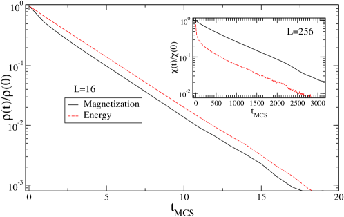
Figure 1: Magnetization and energy autocorrelation functions versus time (in $MCS$) for the Niedermayer algorithm with $E_{0}=0.3$ (see text). The main graph represents the behavior for linear size $L=16$, while the inset applies to $L=256$.

4 Results and Discussion

4.1 Ising model

We first present our results for the Ising model and leave to the next subsection the discussion of the results for the $XY$ model.

As already discussed, the case $E_{0}=-1$ corresponds to the Metropolis algorithm. At the critical temperature, the autocorrelation time scales with $L$ as $\tau\sim L^{z}$, with $z=2.1665\pm 0.0012$ [7]. We have simulated this case only as a test for our algorithm. The value we found for $z$ is consistent with the one quoted above and the scaling law is obeyed, even for the smallest values of $L$ we simulated. Note also that, for the Metropolis algorithm ($E_{0}=-1$), it is the magnetization autocorrelation time which is well described by a single exponential.

The first non-trivial value of $E_{0}$ we simulated was $-0.9$. In Fig. 2 the autocorrelation times for the magnetization is depicted as function of $L$. We note that, for this value of $E_{0}$, only the autocorrelation function for the magnetization is well described by a single exponential. The initial decay of the corresponding function for the energy has an abrupt drop for small times.Therefore, it is not a reliable quantity to extract the autocorrelation time from. The value of $z$ was obtained from the curve for the magnetization and its value is $z=2.16\pm 0.04$, which is, within error bars, the same value as for the Metropolis algorithm.

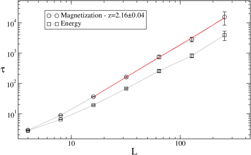
Figure 2: Log-log graphs of magnetization (○) and energy (□) autocorrelation time (in $MCS$) versus linear size $L$ for the Niedermayer algorithm with $E_{0}=-0.9$. The quoted value for $z$ is obtained from the slope of an adjusted straight line for the magnetization autocorrelation time for $L\geq 16$ (see text). The dotted line is just a guide to the eye.

In Fig. 3 the behavior of the mean size of the clusters of spins, $<n>$, is shown, as function of $L$. For this value of $E_{0}$, it seems that $<n>$ does not change with $L$. We will see shortly that in fact it initially grows with $L$ and eventually saturates at some value of $L$, which we call $\widetilde{L}$.

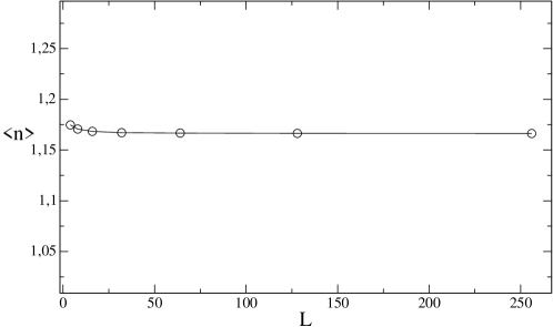
Figure 3: Mean size of the clusters of possibly flipped spins as function of the linear size $L$ for $E_{0}=-0.9$.

The overall picture does not change for $E_{0}=-0.5$: the magnetization autocorrelation function is well described by a single exponential law and the autocorrelation time was calculated from it. The dynamic exponent is $z=2.12\pm 0.03$, still consistent with the Metropolis value (the error bars we quote are all one standard deviation; the intersection with the expected value for the Metropolis algorithm, for this case, is obtained assuming two standard deviations for the error). Since the picture for $E_{0}=-0.5$ does not change from the one for $E_{0}=-0.9$, we will not depict the graphs for the former.

For $E_{0}=0$, a crossover clearly takes place, as shown in Fig. 4: for small $L$, the energy autocorrelation times are larger than their magnetization counterparts, while the situation is reversed for larger $L$ (this behavior is more evident for $E_{0}=0.3$; we showed the corresponding graph in Fig. 1 above and will comment on it below). The value of $z$ is obtained from the slope of an adjusted straight line for the magnetization autocorrelation function, for values of $L$ beyond the point where the crossover takes place. It reads $z=2.15\pm 0.01$ in this case, again compatible with the Metropolis value. The behavior of $<n>$ is shown in Fig. 5: it grows initially with $L$ but eventually saturates at $\widetilde{L}\sim 15$. For small values of $L$ it is the autocorrelation function for the energy which is well described by a single exponential, while the corresponding function for the magnetization shows an abrupt drop for small times. The situation is reversed for $L>\widetilde{L}$.

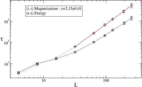
Figure 4: Log-log graphs of magnetization (○) and energy (□) autocorrelation time (in $MCS$) versus linear size $L$ for the Niedermayer algorithm with $E_{0}=0.0$. The quoted value for $z$ is obtained from the slope of an adjusted straight line for the magnetization autocorrelation time, for values of $L$ beyond the point where the crossover takes place. The dotted line is just a guide to the eye.

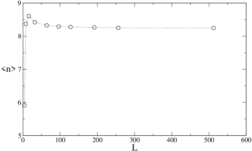
Figure 5: Mean size of the clusters of possibly flipped spins as function of the linear size $L$ for $E_{0}=0.0$.

This picture is maintained for $E_{0}>0.0$, with the value of $\widetilde{L}$ increasing with $E_{0}$ and the crossover taking place at larger and larger values of $L$. The dynamic exponent $z$ is given by $2.16\pm 0.03$ and $2.12\pm 0.04$ for $E_{0}=0.3$ and $0.5$, respectively. Both are compatible with the value for the Metropolis algorithm.

In Fig. 1 we show the change in the behavior of the autocorrelation functions for the magnetization and the energy. Note that the crossover mentioned above is connected also to the possibility of describing the autocorrelation function by a single exponential: this is accomplished by the energy autocorrelation function for small values of $L$ and for its magnetization counterpart for larger values of $L$.

Finally, for $E_{0}=0.7$ and $0.9$ the crossover happens at values of $L$ large enough to prevent a reliable estimate of $z$. It is necessary to go to values of $L$ well above our present computational capabilities to be able to extract $z$ from the graphs.

Nevertheless, the overall trend is well determined: for $0\leq E_{0}<1$, the dynamic behavior is the Metropolis’ one but this behavior sets in only for large enough $L$. The size of the clusters of turned spins increases with $E_{0}$ but eventually saturates for $L=\widetilde{L}$, where $\widetilde{L}$ increases with $E_{0}$. For $L>\widetilde{L}$, the relative size of the clusters (i.e, the ratio $<n>/L^{2}$) decreases and, in this sense, the algorithm is like a single-spin one (Metropolis, in our case), explaining the value of its dynamic exponent. Therefore, the Wolff algorithm (corresponding to $E_{0}=1$) is still the best choice, when compared to the Niedermayer algorithm with $E_{0}<1$.

We postpone the discussion of the Wolff algorithm and go to $E_{0}>1$ . In this case, spins in different states may be part of the same cluster, although with a smaller probability than spins in the same state, and a cluster will always be flipped (see $(iii)$ on page $2$). For $E_{0}\gg 1$, almost all spins in the finite lattice will take part in the cluster and the algorithm will not be optimal (in fact, it won’t even be ergodic for $E_{0}\rightarrow\infty$). Therefore, if the Niedermayer algorithm is more efficient than Wolff’s, it should be for $E_{0}$ close to $1$. We, therefore, studied the cases $E_{0}=1.1$ and $1.05$. The results are qualitatively equivalent and in Fig. 6 we show both. Note that the growth of $\tau$ with $L$ is faster than a power law for both values of $E_{0}$. In the inset, we show the corresponding graph for $E_{0}=1.1$: a crossover is also present but the value where it takes place decreases with $E_{0}$ and for $E_{0}=1.1$ it is not seen. Since the value of the autocorrelation time is already greater then for the Wolff algorithm, for a given $L$, and it grows faster than a power law with $L$, again the optimal algorithm is Wolff’s.

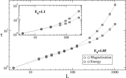
Figure 6: Log-log graphs of magnetization and energy autocorrelation time (in $MCS$) versus linear size $L$ for the Niedermayer algorithm with $E_{0}=1.05$ and $E_{0}=1.1$ (inset). In both graphs the autocorrelation time $\tau$ is plotted as function of the linear size $L$. The dotted line is just a guide to the eye.

We single out the discussion of the Wolff algorithm ($E_{0}=1$), in order to compare with other values of $E_{0}$. Although our intention is not to calculate a precise value of $z$ for this algorithm, we have adjusted the autocorrelation time for the energy (in this case, it is this function which is well described by a single exponential for small values of the time) as a function of $L$ for three different functions, namely:

$$\tau=\left\{\begin{array}[]{l}AL^{z}\\ A\ln L+C\\ A(\ln L)^{z}+C\end{array}\right.$$ (10)

The first function is the usual scaling law assumed for the autocorrelation function at the critical point. We can see in Fig. 7 that there is no indication that the best adjusted curve will eventually be a straight line, in a log-log plot. Since previous calculations tend to point to a value of $z$ close to zero for the Wolff algorithm in two dimensions, one cannot exclude the possibility of a logarithmic dependence, which is the case of the second function in the above equation. The fitting is better than for the power law but it is not a satisfactory one either. Moreover, it tends to deviate from the data for large enough $L$. The third function is an ad hoc assumption, which proved to be the best fit to our data, as can be seen in Fig. 7. The parameters of the function are obtained from a non-linear fitting:

$$\tau=A(\ln L)^{z}+C,$$ (11)

with $A=0.21\pm 0.01$, $z=1.50\pm 0.02$ e $C=0.47\pm 0.03$. We have no theoretical explanation for this behavior. The constant $C$, however, is a finite-size correction. The behavior in Eq. 11 is expected to hold true for large enough $L$ and the logarithmic dependence makes the scaling region to be reached only for very large values of $L$. For this region, one would expect a simpler law, namely $\tau=A(\ln L)^{z}$; however, for intermediate or small values of $L$, the constant $C$ acts as a finite-size correction. A similar scaling law was found for the exponential relaxation time for the Swendsen-Wang algorithm [13].

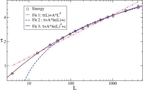
Figure 7: Log-log graph of the energy autocorrelation time (in $MCS$) as a function of $L$ for the Wolff algorithm. The three fitted curves proposed in 10 are showed.

We also depict the mean size of the clusters of turned spins, $<n>$, as a function of $L$ in Fig. 8. The slope of the straight line is $1.7500\pm 0.0001$, which is, as expected [2], the value for the ratio $\gamma/\nu$. Note that, contrarily to what happens for $E_{0}<1$, there is no saturation of $<n>$ with $L$. This seems to explain why Wolff and Niedermayer algorithms are in different dynamic universality classes.

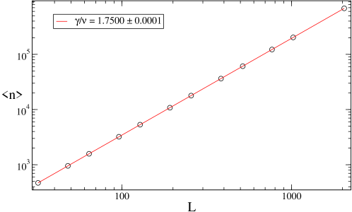
Figure 8: Log-log graph of the mean size of turned clusters as function of $L$. The slope is an evaluation of $\gamma/\nu$.

4.2 XY model

We have applied the Niedermayer algorithm in the study of the dynamic behavior of the $XY$ model as well. The generalization of this algorithm to continuous models is outlined in the Appendix. Although we have studied three values of $E_{0}$, our results are conclusive and lead to an overall picture which is analogous to the one for the Ising model. We have used the value $k_{B}T_{c}/J=0.8865$ for the transition temperature of the two-dimensional $XY$ model. This value is only $0.7\%$ off of the most recent evaluation of $k_{B}T_{c}/J$ for this model [14].

The mean size of the clusters of flipped spins for the Wolff algorithm as a function of the linear size of the lattice is depicted in Fig. 9. The slope of the straight line is $1.7454\pm 0.009$, which is slightly different from the expected value for $2-\eta$ for this model at $k_{B}T_{c}/J$, $7/4$ [15]. In fact, the small discrepancy may be due to the fact that we are not using the (unknown) exact value for the transition temperature.

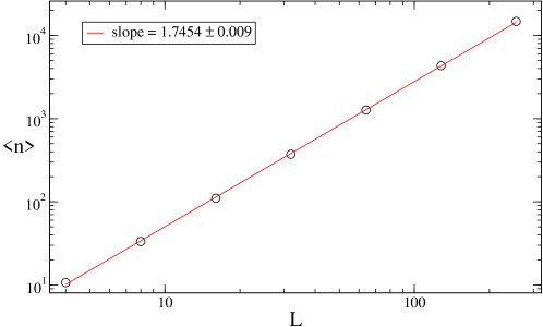
Figure 9: Log-log plot of the mean size of the clusters of flipped spins for the $XY$ model versus the linear size of the lattice. The slope of the curve just misses the expected value for $2-\eta$, $7/4$ [15].

The autocorrelation times for the magnetization and energy for the Wolff algorithm are shown in Fig. 10. We have not tried to fit the data but it is evident that the energy autocorrelation time grows with $L$ slower than a power law. The decrease in the magnetization autocorrelation time has been observed previously (in fact, an oscillation was observed in an algorithm which mixed Wolff’s and Swendsen-Wang’s procedures but the overall picture is qualitatively similar to ours; see Ref.[16]).

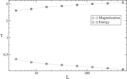
Figure 10: Autocorrelation times for the magnetization (circle) and energy (square) for the Wolff algorithm applied to the two-dimensional $XY$ model.

We have simulated also the cases $E_{0}=0$ and $E_{0}=-0.5$. The mean size of clusters of flipped spins saturates and the value of saturation increases with $E_{0}$ (see Fig. 11). Therefore, one expects the same picture as for the Ising model: in particular, the dynamic behavior for $L$ large enough is the Metropolis’ one. This is confirmed for $E_{0}=0.0$ explicitly, where the dynamic exponent measured is $z=1.916\pm 0.004$ (see Fig. 12). Recalling our reasoning for the Ising model for $E_{0}<1$, we can infer that the value just quoted for $z$ is an evaluation of the dynamic exponent for the Metropolis algorithm applied to the two-dimensional $XY$ model. Since, to the best of our knowledge, there is no previous evaluation of $z$ for this model and for the Metropolis algorithm, we have made a crude evaluation of $z$ for this case and obtained the value $1.89\pm 0.03$, which is in agreement, within error bars, with the value we obtained for $E_{0}=0.0$ for large $L$. Clearly, the Wolff algorithm is the most efficient, when compared to the Niedermayer algorithm with the two values of $E_{0}$ quoted above. We have also simulated one example of $E_{0}>1$, namely $E_{0}=1.05$. The behavior is qualitatively the same as for the Ising model; see Fig. 13. Note that the growth of the autocorrelation time is faster than a single power law; in fact, it is well fitted by an exponential. Therefore, also for the $XY$ model the best choice is $E_{0}=1$ (Wolff algorithm), when compared to the Niedermayer algorithm.

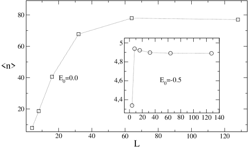
Figure 11: Mean size of the clusters of flipped spins for $E_{0}=-0.5$ (inset) and $E_{0}=0$ (main graph) for the two-dimensional $XY$ model.

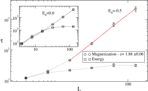
Figure 12: Autocorrelation time for the magnetization and energy as a function of $L$ for $E_{0}=-0.5$ (main graph) and $E_{0}=0$ (inset) for the two-dimensional $XY$ model.

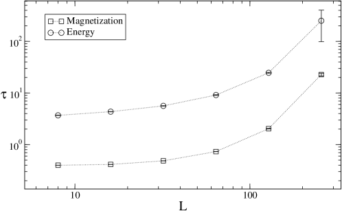
Figure 13: Autocorrelation time for the magnetization and energy as a function of $L$ for $E_{0}=1.05$ for the two-dimensional $XY$ model.

5 Summary

We have studied the dynamic behavior of the Niedermayer algorithm applied to the two-dimensional Ising and $XY$ models. Our main goal is to compare its efficiency with the Wolff algorithm’s. The latter is a particular case of the Niedermayer algorithm, such that a parameter governing the size of the flipped clusters, $E_{0}$, assumes the value $1$.

We show that, for $-1<E_{0}<1$, the dynamic behavior eventually recovers the Metropolis’ ($E_{0}=-1$) one. This behavior is linked to the saturation of the mean size of the clusters, which happens for all $E_{0}<1$, leading to a decrease of the relative size of these clusters when $L$ increases.

For the Wolff algorithm and the Ising model, we propose an scaling function for the autocorrelation time for the magnetization. This choice is an ad hoc one but fits the data very well and does not coincide with any function proposed so far in the literature. We were not able to make a fitting with the same statistical quality for the $XY$ model.

For $E_{0}>1$, the values of the autocorrelation times are greater than those for the Wolff algorithm and grow faster than a power law with $L$.

Therefore, at least for these two models, the Wolff algorithm is superior to Niedermayer’s.

6 Appendix

The Hamiltonian for the XY model can be written as:

$$\mathcal{H}=-J\sum_{<i,j>}\vec{s_{i}}\cdot\vec{s_{j}}$$ (12)

where $J$ is the coupling constant and $\vec{s_{i}}$ is the spin of site $i$, represented by a unit vector in any direction in the $xy$ plane.

To start the cluster we randomly choose a preferred direction $\hat{n}$ and a spin $\vec{s_{i}}$. This spin is the first one of the cluster. Neighbours of $\vec{s_{i}}$ are added to cluster with probability:

$$P_{add}=\left\{\begin{array}[]{ll}1-e^{KE_{ij}\left(1+E_{0}\right)},&\mbox{if}\;\;E_{ij}<E_{0},\\ 0,&\mbox{otherwise},\end{array}\right.$$ (13)

where in the XY model, $E_{ij}=-(\vec{s_{i}}\cdot\hat{n})(\vec{s_{j}}\cdot\hat{n})$. Note that, if $E_{0}\leq 1$, only sites that have the same component in the direction $\hat{n}$ as $\vec{s_{i}}$ may be added to the cluster. The procedure for the construction of the cluster continues as described for the Ising model. After the cluster is built the new directions of the spins are given by a reflection with respect to axis perpendicular to $\hat{n}$.

The acceptance ratio for XY model is slightly different from the one for the Ising model. We cannot define the energy difference ($\Delta E$) as the number of parallel and anti-parallel spins to the cluster. So we must calculate the energy before and after the cluster is flipped. In this case we define de acceptance ratio, for $E_{0}\leq 1$, as:

$$A(a\rightarrow b)={\Bigg{\{}}\begin{array}[]{cc}e^{-\frac{\Delta E}{2}K(1-E_{0})},&\mbox{if}\;\;\;\Delta E>0\\ 1\;\;\;\;\;\;\;\;\;\;\;\;\;\;\;\;\;\;\;\;\;,&\mbox{if}\;\;\;\Delta E<0,\end{array}$$ (14)

where $a$ and $b$ have the same meaning as before and $\Delta E$ is the difference in energy between configurations $a$ and $b$, in units of $J$. As we can see, for $E_{0}=-1$ we regain the Metropolis algorithm with $A=e^{-K\Delta E}$ and for $E_{0}=1$ we regain the Wolff algorithm with $A=1$ for all clusters. These choices ensure that detailed balance is obeyed.

The generalization for $E_{0}>1$ is analogous to the one described above and, again, spins with different signs for the component along $\hat{n}$ may also be part of the cluster and $A=1$ always.

References

References

- [1] David P. Landau and Kurt Binder. A Guide to Monte Carlo Simulations in Statistical Physics. Cambridge University Press, New York, USA, second edition, 2005.
- [2] M. E. J. Newman and G. T. Barkema. Monte Carlo Methods in Statistical Physics. Oxford University Press, Oxford, UK, 2001.
- [3] F. G. Wang and D. P. Landau. Phys. Rev. Lett., 86:2050, 2001.
- [4] P. M. C. de Oliveira. Computing Boolean Statistical Models. World Scientific, London, UK, 1991.
- [5] R. H. Swendsen and J.-S. Wang. Phys. Rev. Lett., 58:86, 1987.
- [6] U. Wolff. Phys. Rev. Lett., 62:361, 1989.
- [7] M. P. Nightingale and H. W. Bl te. Phys. Rev. Lett., 76:4548, 1996.
- [8] C.F. Baillie and P.D. Coddington. Phys. Rev. B, 43(13):10617, 1991.
- [9] P. D. Coddington and C. F. Baillie. Phys. Rev. Lett., 68:962, 1992.
- [10] F. Niedermayer. Phys. Rev. Lett., 61:2026, 1988.
- [11] S. Wansleben and D. P. Landau. Phys. Rev. B, 43:6006, 1991.
- [12] J. Salas and A. D. Sokal. J. of Stat. Phys., 87:1, 1997.
- [13] J. Du, B. Zheng, and J.-S. Wang. Journal of Statistical Mechanics: Theory and Experiment, 2006:P05004, 2006.
- [14] H. Arisue. Progr. Theor. Phys., 118:855, 2007.
- [15] P. Butera and M. Percini. Physica A, 387:6293, 2008.
- [16] R. G. Edwards and A. D. Sokal. Phys. Rev. D, 40:1374, 1989.