Abstract

Interacting quantum scalar field theories in $dS_{D}\times M_{d}$ spacetime can be reduced to Euclidean field theories in $M_{d}$ space in the vicinity of $I_{+}$ infinity of $dS_{D}$ spacetime. Using this non-perturbative mapping, we analyze the critical behavior of Euclidean $\lambda\phi_{4}^{4}$ theory in the symmetric phase and find the asymptotic behavior $\beta(\lambda)\sim\lambda$ of the beta function at strong coupling. Scaling violating contributions to the beta function are also estimated in this regime.

1 Introduction

Almost 35 years ago Wilson and Kogut [1] have suggested that the $\lambda\phi_{d}^{4}$ quantum field theory is in fact trivial in number of dimensions $d\geq 4$, e.g., the renormalized coupling $\lambda(p)$ vanishes at small momenta $p$ for any finite bare coupling $\lambda_{0}$ and the correlation properties of the field $\phi$ become Gaussian. The question whether the theory is trivial in this sense is not merely academic: one of the strongest theoretical upper bounds on the value of the Higgs mass $m_{H}$ comes from the fact that the quantum field theory of the Higgs field coupled to non-Abelian gauge theory describing weak interaction is either trivial or asymptotically free depending on the value of $m_{H}$ [3].

Triviality of the theory in $d\geq 5$ dimensions was rigorously established [7, 8] using the representation of Euclidean field theories as systems of random currents (essentially world lines of elementary excitations in the first quantized version of the theory), but the case $d=4$ turned out to be special and much more complicated [4, 5]. Although the validity of the Wilson conjecture in this case is supported by results of lattice simulations [6], to this day there exists no strict proof of triviality of the $\lambda\phi_{4}^{4}$ theory.

Let us recall why the $d=4$ case is so special in both the field theoretic framework and the geometric picture of random currents. In the latter, triviality is equivalent to the statement that two random Brownian paths generically do not intersect. As it turns out, the probability of such an intersection is indeed zero if Brownian paths are located in space with number of dimensions higher than $4$. In $d=4$ dimensions, the geometry of a random walk is more complicated: although the probability for two Brownian paths to intersect is zero, the probability for both of them to penetrate a ball of the radius $\epsilon$ is $1$ for any, even infinitely small, value of $\epsilon$.

In the field theoretic framework, the triviality of $\lambda\phi_{4}^{4}$ theory is directly related to the existence of a non-perturbative Landau pole. The 1-loop renormalization law

$$\lambda(p^{\prime})=\frac{\lambda(p)}{1-\frac{3\lambda^{2}(p)}{16\pi^{2}}\log\frac{p^{\prime}}{p}},$$ (1.1)

featuring a singularity at finite momentum $p^{\prime}\sim p\cdot\exp\left(\frac{16\pi^{2}}{3\lambda^{2}(p)}\right)$, implies that the renormalized coupling vanishes at small momenta for any finite value of the bare coupling $\lambda_{0}$. On the other hand, since one expects the coupling $\lambda$ to grow in the vicinity of the Landau pole, the validity of the 1-loop approximation for the beta function

$$\beta(\lambda)=\frac{3}{16\pi^{2}}\lambda^{2}$$ (1.2)

breaks down. It is not completely clear whether the Landau pole survives at the non-perturbative level. The alternative to the runaway behavior (1.1) would be the existence of a non-perturbative UV fixed point(s) and, as a consequence, asymptotic freedom at very large momenta. Results of lattice simulations seem to disfavor such a scenario [6].

In the absence of UV fixed points, one expects that the perturbative formulation of the $\lambda\phi_{4}^{4}$ theory is UV incomplete since it is impossible to probe the theory at arbitrarily large momenta. A question appears in this context whether it is possible to find an embracing “fundamental” theory which at small momenta reduces to the strongly coupled $\lambda\phi_{4}^{4}$ theory with $\lambda(p)\gg 1$ and negligible scaling violation corrections [4]. In the present work we address this question and present a corresponding embracing theory explicitly. We find the asymptotic behavior $\beta(\lambda)\sim\lambda$ at large values of the renormalized coupling, implying that the Landau pole is absent at the non-perturbative level.

The paper is organized as follows. In the Sections 2 and 3 we study correlation properties of scalar quantum field theories in $dS_{D}\times M_{d}$ spacetime, where $M_{d}$ is a $d$-torus or $d$-dimensional non-compact flat Euclidean space. We find that the Nicolai map is naturally generated for such theories relating the large scale (superhorizon) scalar field $\Phi$ and the “random force” composite operator - a superposition of modes with physical wavelength of the order of the $dS$ horizon size. Using the Nicolai map we explicitly derive a correspondence between self-interacting scalar QFTs in $dS_{D}\times M_{d}$ spacetime and Euclidean field theories in $M_{d}$ target space: the former are reduced to the latter in the vicinity of the $I_{+}$ infinity of de Sitter space.

This is an important byproduct of our study. In a sense, the correspondence between field theories in $dS_{D}\times M_{d}$ and $M_{d}$ spaces means that de Sitter space provides a natural geometric framework for stochastic quantization of a self-interacting Euclidean scalar field theory in $d$-dimensional space. The procedure of stochastic quantization first introduced by Parisi and Wu to analyze correlation properties of Euclidean gauge theories without gauge fixing [9], has led to development of new effective algorithms for lattice QFT simulations, advances in study of large $N$ theories and master fields, etc. [10] Recently, it was discovered that several apparently unrelated QFTs such as the Wess-Zumino-Novikov-Witten model and the strong coupling limit of topologically massive Yang-Mills theory are actually connected via stochastic quantization [11]. It would be interesting to understand in this context whether the developed geometric framework for stochastic quantization implies the existence of a field theory/gravity duality relating the field theories listed in [11].

In the Section 4, the derived correspondence is used to study critical properties of $\lambda\phi_{4}^{4}$ theory. It allows us to introduce a UV completion of $\lambda\phi_{4}^{4}$ theory such that its correlation properties at large momenta are governed by a higher dimensional theory. We estimate the beta function of the theory at strong coupling and argue that $\lambda\phi_{4}^{4}$ theory is a “marginal” case between trivial $\lambda\phi_{d}^{4}$ theories with $d>4$ and theories with $d\leq 4$. The beta function of the theory behaves as

$$\beta(\lambda)\sim\lambda$$ (1.3)

at strong coupling $\lambda\gg 1$ and, as a result, the renormalized coupling $\lambda(\Lambda)$ diverges as $\Lambda\to\infty$ although the non-perturbative Landau pole is absent. Our framework also allows us to estimate scaling violating corrections to the beta function. We find that they are typically large in the regime where the asymptotics (1.3) is applicable. Finally, Section 5 is devoted to the discussion.

2 De Sitter space as stochastic quantization machine

Let us consider a massive self-interacting scalar field theory with Langrangian density

$${\cal L}=\frac{1}{2}(\partial\phi)^{2}-\frac{1}{2}m^{2}\phi^{2}-\frac{1}{4!}\lambda\phi^{4},$$ (2.1)

in a $dS_{D}\times M_{d}$ spacetime. Here by $dS_{D}$ we understand a $t\in[0,+\infty)$ part of the planar patch of the $D$-dimensional de Sitter space covered by a coordinate system $(t,\mathbf{x})=(t,x_{1},\ldots,x_{D-1})$ with metric

$$ds^{2}=dt^{2}-a^{2}(t)\sum_{i=1}^{D-1}dx_{i}dx^{i}$$ (2.2)

and scale factor $a(t)\sim\exp(Ht)$. The $d$-dimensional Euclidean space $M_{d}$ is either a torus $T_{d}$ or non-compact flat space $E_{d}$ covered by a coordinate system $\mathbf{y}=(y_{1},\ldots,y_{d})$. The Hubble constant $H$ is related to the curvature of $dS_{D}$ spacetime by $R=D(D-1)H^{2}$. In what follows, we neglect the backreaction of the scalar field on background spacetime, considering only the limit $M_{P}\to\infty$.

The dynamics of quantum Heisenberg operator $\phi(t,\mathbf{x},\mathbf{y})$ is determined by the equation of motion

$$\ddot{\phi}+(D-1)H\dot{\phi}-\frac{\nabla_{x}^{2}}{a^{2}}\phi-\nabla_{y}^{2}\phi+m^{2}\phi+\frac{1}{6}\lambda\phi^{3}=0.$$ (2.3)

It is convenient to decompose the Heisenberg operator $\phi(t,\mathbf{x},\mathbf{y})$ into ultraviolet (subhorizon) and infrared (superhorizon) contributions [14, 15] according to the prescription

$$\phi=\Phi+\int\frac{d^{d}p}{(2\pi)^{d/2}}\frac{d^{D-1}k}{(2\pi)^{\frac{D-1}{2}}}\theta(k-\epsilon aH)\left(a_{k,p}f_{k,p}(t)e^{-i\mathbf{(k}\mathbf{x}+\mathbf{py})}+a_{k,p}^{\dagger}f_{k,p}^{*}(t)e^{i(\mathbf{kx}+\mathbf{py})}\right)+\delta\phi,$$ (2.4)

where $\theta(x)$ is the Heaviside step function, $\epsilon$ is a free parameter,

$$f_{k,p}(t)=\frac{\sqrt{-\pi\eta}}{2a^{\frac{D-2}{2}}}H_{\frac{D-1}{2}}^{(1)}(-k\eta)e^{\frac{i\pi D}{4}}$$ (2.5)

are modes of a free massless scalar field in $dS_{D}$ background ($\eta=-\frac{1}{Ha(t)}$ is conformal time) and $\delta\phi$ is a contribution of the order ${\cal O}\left({\rm max}\left(\frac{m^{2}}{H^{2}},\frac{\lambda\langle\phi^{2}\rangle}{H^{2}}\right)\right)$. In order for the contribution $\delta\phi$ to be negligible, $\epsilon$ should satisfy the condition

$$\exp\left(-\frac{(D-1)H^{2}}{m_{{\rm eff}}^{2}}\right)\ll\epsilon\lesssim 1,$$ (2.6)

where $m_{{\rm eff}}^{2}=m^{2}+3\lambda(H)\langle\phi^{2}\rangle$ [14]. An estimation for the Hartree mass and bounds for renormalized coupling will be given below.

In the leading order approximation in small “slow roll” parameters $\frac{m^{2}}{H^{2}},\,\frac{\lambda\langle\phi^{2}\rangle}{H^{2}}$, the equation of motion for the infrared part $\Phi(t,\mathbf{x},\mathbf{y})$ of the Heisenberg operator $\phi(t,\mathbf{x},\mathbf{y})$ acquires the form

$$\dot{\Phi}=-\frac{1}{(D-1)H}(\nabla_{y}^{2}+m^{2})\Phi-\frac{1}{6(D-1)H}\lambda\Phi^{3}+f(t,\mathbf{x},\mathbf{y}),$$ (2.7)

where

$$f(t,\mathbf{x},\mathbf{y})=\frac{\epsilon H^{2}}{(2\pi)^{(D+N-1)/2}a^{(D-4)/2}}\int d^{d}p\,d^{D-1}k\,\delta(k-\epsilon aH)\frac{i}{\pi}\Gamma\left(\frac{D-1}{2}\right)\times$$

$$\times\left(-\frac{2}{k\eta}\right)^{\frac{D-1}{2}}\sqrt{-\frac{\pi\eta}{4}}\left(a_{k}e^{-ikx-ipy}e^{\frac{i\pi D}{4}}-a_{k}^{\dagger}e^{ikx+ipy}e^{-\frac{i\pi D}{4}}\right).$$ (2.8)

The composite operator $f(t,\mathbf{x},\mathbf{y})$ has correlation properties of white noise

$$\langle f(t,\mathbf{x},\mathbf{y})f(t^{\prime},\mathbf{x},\mathbf{y}^{\prime})\rangle=\frac{\Gamma\left(\frac{D-1}{2}\right)}{2\pi^{\frac{D+1}{2}}}H^{D-1}\delta(t-t^{\prime})\delta^{d}(\mathbf{y}-\mathbf{y}^{\prime}),$$ (2.9)

where average above is in the Bunch-Davies vacuum state. These correlation properties do not depend on the parameter $\epsilon$ in the decomposition (2.4) if the operators $f(t,\mathbf{x},\mathbf{y})$ and $f(t^{\prime},\mathbf{x},\mathbf{y}^{\prime})$ are taken at the same point $\mathbf{x}$ (or, more precisely, within the same Hubble patch) of the de Sitter space $dS_{D}$. Another important property of equation (2.7) is that all terms in it commutate with each other, and therefore the large scale field $\Phi$ can be considered a classical quantity [14]. Thus, the equation (2.7) is a Langevin equation describing a random walk of the classical large scale field $\Phi$.

Its physical meaning can be understood as follows. An observer living in $dS_{D}\times M_{d}$ space cannot discriminate between different modes with physical wavelengths $\lambda\sim\frac{a}{k}$ larger than the scale of cosmological horizon $H^{-1}$ and interprets their collection as a classical background field $\Phi(t)$. The value of $\Phi(t)$ changes, while more and more modes leave the cosmological horizon (a mode $f_{k}$ with momentum $k$ leaves the horizon at the moment of time $t$ such that $a(t)\sim\frac{k}{H}$). This picture is known to describe the phenomenon of eternal (stochastic) inflation [17].

The Langevin equation (2.7) is analogous to the one appearing in the procedure of stochastic quantization for a $D$-dimensional quantum scalar field theory with potential $V(\phi)=\frac{1}{2}m^{2}\phi^{2}+\frac{1}{4!}\lambda\phi^{4}$, implying that the late time behavior of the correlation functions of the field $\phi$ propagating in $(D+d)$-dimensional $dS_{D}\times M_{d}$ spacetime is effectively determined by a $d$-dimensional theory. One can say that for any interacting scalar field $\phi$, de Sitter space “generates” a Nicolai map [18] from the field propagating in the bulk of $dS_{D}$ to the same field at the boundary (horizon), since the “random force” operator $f(t,\mathbf{x},\mathbf{y})$ is a linear combination of modes $\delta\phi_{k}$ with momenta $k=aH$ (2.8).

We will now show how to construct the partition function of the corresponding $d$-dimensional theory explicitly. The Fokker-Planck equation describing evolution of the probability $P(\Phi(t,\mathbf{y}),t)$, which measures a given value of the large scale field $\Phi$ in a given Hubble patch, has the form

$$\frac{\partial P}{\partial t}=\hat{H}P=\int d^{d}y\frac{\delta}{\delta\Phi}\left(A\frac{\delta}{\delta\Phi}+B(\nabla_{y}^{2}+m^{2})\Phi+\frac{\lambda B}{6}\Phi^{3}\right)P,$$ (2.10)

where

$$A=\frac{H^{D-1}}{4\pi^{\frac{D+1}{2}}}\Gamma\left(\frac{D-1}{2}\right),\,\,B=\frac{1}{(D-1)H}.$$ (2.11)

In order to illustrate several important properties of its general solution, let us first perform a Fourier transform along the directions in $M_{d}$ and neglect the self-interaction of the field $\Phi$, setting $\lambda=0$ so that Kaluza-Klein modes with different momenta $p$ become decoupled from each other. The Fourier mode $P_{p}$ of the probability distribution $P$ is given by

$$P_{p}(\Phi_{p},t)=\exp\left(-\frac{B}{4A}(p^{2}+m^{2})\Phi_{p}^{2}\right)\sum_{n=0}^{\infty}c_{n}\psi_{n}(\Phi_{p})e^{-2AE_{n}(t-t_{0})},$$ (2.12)

where $\psi_{n}(\Phi_{p})$ and $E_{n}$ are eigenfunctions and eigenvalues of the Schrodinger equation

$$-\frac{1}{2}\psi_{n}^{\prime\prime}+\frac{(p^{2}+m^{2})^{2}B^{2}}{8A^{2}}\psi_{n}=\tilde{E}_{n}\psi_{n}=\left(E_{n}+\frac{B(p^{2}+m^{2})}{4A}\right)\psi_{n}.$$ (2.13)

All eigenvalues $E_{n}$ are non-negative and the lowest eigenstate has zero energy $E_{0}=0$, since the Hamiltonian in (2.10) is supersymmetric [14]. Therefore, all Fourier modes of the probability distribution $P$ have finite asymptotics

$$P_{p}(\Phi_{p})=\exp\left(-\frac{B}{2A}(p^{2}+m^{2})\Phi_{p}^{2}\right)$$ (2.14)

at $t\to\infty$, e.g., in the vicinity of future infinity $I_{+}$ of de Sitter space. After performing an inverse Fourier transformation, we finally find that the asymptotic probability to measure a given value of the classical field $\Phi(\mathbf{y})$ in a given Hubble patch and at a given point $\mathbf{y}$ in the extra dimensions is

$$P(\Phi)=\prod_{p}P_{p}(\Phi_{p})=\exp\left(-\frac{C}{2}\int d^{d}y((\nabla_{y}\Phi)^{2}+m^{2}\Phi^{2})\right),$$ (2.15)

where

$$C=\frac{4\pi^{\frac{D+1}{2}}H^{-D}}{(D-1)\Gamma\left(\frac{D-1}{2}\right)},$$ (2.16)

or, introducing a new variable $\chi=\sqrt{C}\Phi$,

$$P(\chi)=\exp\left(-\frac{1}{2}\int d^{d}y((\nabla_{y}\chi)^{2}+m^{2}\chi^{2})\right).$$ (2.17)

Similarly, one can show that, when self-interaction is taken into account,

$$P(\chi)=\exp\left(-\frac{1}{2}\int d^{d}y((\nabla_{y}\chi)^{2}+m^{2}\chi^{2}+\frac{1}{12}\tilde{\lambda}\chi^{4})\right),$$ (2.18)

where

$$\tilde{\lambda}=\frac{\lambda}{C}=\frac{(D-1)\Gamma\left(\frac{D-1}{2}\right)}{4\pi^{\frac{D+1}{2}}}\lambda H^{D}.$$ (2.19)

The correlation properties of the classical field $\chi(\mathbf{y})$ are calculated as in Euclidean field theory with partition function

$$Z\{\chi\}=\int{\cal D}\chi\exp\left(-\frac{1}{2}\int d^{d}y((\nabla_{y}\chi)^{2}+m^{2}\chi^{2}+\frac{1}{12}\tilde{\lambda}\chi^{4})\right)$$ (2.20)

We conclude that in the vicinity of the $I_{+}$ infinity, the interacting scalar field theory in $dS_{D}\times M_{d}$ spacetime is reduced to a Euclidean field theory of a field $\chi$ in $M_{d}$ manifold in the sense that the probability to measure a given value of the classical field $\Phi(\mathbf{y})$ in a given Hubble patch and at a point $\mathbf{y}$ in the extra dimensions is determined by the partition function (2.20).

Apart from the inverse correlation length $m_{{\rm ren}}$, there are two scales of interest in the theory: $\frac{1}{2}\sqrt{D(D-2)}H\sim\frac{1}{2}DH$ and $\sqrt{2}H$. The inverse curvature radius of $dS_{D}$ space $R_{dS}^{1/2}\sim DH$ plays the role of an ultraviolet cutoff for the theory (2.20), since only the modes with sufficiently low momenta $p$ along the extra dimensions can contribute to the partition function (2.20).

To prove this statement, let us consider the equation of motion for the modes $u_{k,p}=f_{k,p}a^{\frac{D-2}{2}}$ of a massive scalar field on a $dS_{D}\times M_{d}$ background

$$u_{k,p}^{\prime\prime}+\left(k^{2}-\frac{D(D-2)-4(p^{2}+m^{2})/H^{2}}{4\eta^{2}}\right)u_{k,p}=0,$$ (2.21)

where prime denotes differentiation w.r.t. conformal time $\eta=-\frac{1}{Ha(t)}$. The infrared effect we are after (build up of the coherent large scale field $\Phi$) is due to the freeze-out of superhorizon modes with $k\ll aH$, when the effective mass of the given mode $u_{k,p}$ becomes negative. For a given $k$ and $p$, the solution of (2.21) is a linear combination of a decaying and a growing mode. In the regime $k\ll aH$, the decaying mode can be neglected compared to the growing mode, so that the dynamics of $u_{k,p}$ becomes quasi-classical. Only those modes contribute to the quasi-classical field $\Phi$, and the evolution of the latter is determined by the Langevin equation (2.7). Apparently, this quasi-classical regime can only be possible for modes with momenta

$$p<\sqrt{p^{2}+m^{2}}\lesssim\frac{\sqrt{D(D-2)}}{2}H=L^{-1}.$$ (2.22)

Therefore, the effective action in the partition function (2.20) is actually coarse-grained at scales $L\sim(DH)^{-1}$ determined by (2.22). One can study the infrared and ultraviolet properties of the theory (2.20) by appropriately modifying this coarse-graining scale.

The inverse Hubble scale $H^{-1}$ is a natural unit for measuring the time and length scales in the problem: it enters into the background metric of spacetime only in the combination $\exp(Ht)$ and defines the cross-correlation between different Hubble patches, since the equal time pair correlation function of the field $\phi(t,\mathbf{x},\mathbf{y})$ has the form [20]

$$\langle\phi(t,\mathbf{x},\mathbf{y})\phi(t,\mathbf{x}^{\prime},\mathbf{y})\rangle\approx\langle\phi(t,\mathbf{x},\mathbf{y})\rangle^{2}\left(1-\frac{1}{Ht}\log H|\mathbf{x}-\mathbf{x}^{\prime}|\right).$$ (2.23)

Also, as we will see in the next Section, the scale $\sqrt{2}H$ provides the fundamental ultraviolet cutoff for the theory in the sense that at $p\lesssim\sqrt{2}H$, it can no longer be described by the partition function (2.20).

3 Physics at large momenta

The partition function (2.20) correctly describes physics of the $\lambda\phi^{4}$ theory in a $dS_{D}\times M_{d}$ spacetime at low physical momenta $\mathbf{p}_{{\rm phys}}^{2}=\frac{k^{2}}{a^{2}}+p^{2}\ll(DH)^{2}$ (and in the limit $a\to\infty$). The UV physics of the theory can be analyzed straightforwardly by considering the behavior of the modes with physical momenta $\mathbf{p}_{{\rm phys}}^{2}=\frac{k^{2}}{a^{2}}+p^{2}\gg(DH)^{2}$. We are particularly interested in determining how this range of physical momenta contributes to the renormalization of $\lambda$.

At $p\gg H$, $k\ll aH$, the behavior of the theory is the same as the large scale behavior of heavy scalar fields in a de Sitter background. It is well known that such fields are not generated. Indeed, in this regime one can rewrite the effective action for the field $\phi$ in terms of the variable $v(t,\mathbf{x},\mathbf{y})=\phi(t,\mathbf{x},\mathbf{y})a^{\frac{D-1}{2}}$, neglecting the $m^{2}\phi^{2}$ term and the dependence of the Lagrangian density on the spatial coordinates $\mathbf{x}$ of $dS_{D}$ space:

$$S\approx\int dtd^{D-1}xd^{d}y\left(\frac{1}{2}(\dot{v})^{2}-\frac{1}{2}(\nabla_{y}v)^{2}-\frac{\lambda v^{4}}{4!a^{D-1}}\right).$$ (3.1)

Therefore, the interval $p\gg H$, $k\ll aH$ only contributes to the renormalization of $\lambda$ at early times $t\lesssim H^{-1}$.

Similarly, one can show that the interval $p\ll H$, $k\gg aH$ (corresponding to light subhorizon modes) only contributes at $t\lesssim H^{-1}$: neglecting the $m^{2}\phi^{2}$ term and the dependence on the coordinates $\mathbf{y}$ in $M_{d}$ space, one can rewrite effective action in terms of the variable $u=\phi a^{\frac{D-2}{2}}$ as

$$S\approx\int d\eta d^{D-1}xd^{d}y\left(\frac{1}{2}(u^{\prime})^{2}-\frac{1}{2}(\nabla_{x}u)^{2}-\frac{\lambda u^{4}}{4!a^{D-4}}\right)$$ (3.2)

and find that the interaction term is again suppressed by powers of the scale factor. This suppression is present only for $D>4$, while at $2\leq D\leq 4$ we lose control over the behavior of the theory at $p\lesssim DH$. This suggests that the scale $\sqrt{2}H$ is the fundamental UV cutoff for the theory.

Finally, at $t\lesssim H^{-1}$ (and for the interval $p\gg H$, $k\gg aH$), when all the modes are still within a single Hubble volume, the expansion of the spacetime can be entirely neglected and the effective action for the field $\phi$ acquires the form

$$S=\int dtd^{D-1}xd^{d}y\left(\frac{1}{2}(\dot{\phi})^{2}-\frac{1}{2}(\nabla_{x,y}\phi)^{2}-\frac{1}{2}m^{2}\phi^{2}-\frac{1}{4!}\lambda\phi^{4}\right).$$ (3.3)

The modes of the theory (3.3) propagate in flat spacetime of dimensionality $D+d>4+d>D_{{\rm cr}}=4$ larger than critical. Therefore, all critical exponents of the theory can be determined using mean field approximation [22]. The $(D+d)$-dimensional theory (3.3) is UV incomplete and should be provided with a UV cutoff scale $\Lambda_{{\rm UV}}$. In the limit $\Lambda_{UV}\to\infty$ the theory (3.3) is trivial [7, 8], so we are naturally interested in the case of finite $\Lambda_{{\rm UV}}$.

In the mean field approximation, the major effect of the interaction term is the Hartree contribution to the effective mass of the field $\phi$, which can be estimated as

$$m_{{\rm eff}}^{2}=3\lambda_{0}\langle\phi^{2}\rangle\approx\frac{3\lambda_{0}\Lambda_{UV}^{D+d-2}}{4(D+d)},$$ (3.4)

where $\lambda_{0}$ is the bare coupling constant. If $\Lambda_{{\rm UV}}$ is sufficiently large, $\lambda\langle\phi^{2}\rangle\gg m^{2}$. In order for the infrared limit (2.20) to exist, the condition $m_{{\rm eff}}^{2}\lesssim L^{-2}=\frac{D(D-2)}{4}H^{2}$ or

$$\lambda_{0}\Lambda_{{\rm UV}}^{D+d-4}\lesssim\frac{4(D+d)}{3}\frac{1}{(\Lambda_{{\rm UV}}L)^{2}},$$ (3.5)

should be satisfied. The physical meaning of this condition is simple: in the theory (2.20) with UV cutoff $L^{-1}$, modes with effective mass larger than the cutoff scale are integrated out.

Non-gaussian contributions to correlation functions of the theory (3.3) are expected to be small in the limit of large $\Lambda_{{\rm UV}}$, since the renormalized 4-point vertex (and the renormalized self-interaction constant $\lambda$) remains uniformly bounded (and vanishes in the limit $\Lambda_{{\rm UV}}\to\infty$) [7, 8] as

$$\lambda_{{\rm ren}}=\frac{|u^{(4)}(p_{i}=0)|}{G^{4}(p=0)}\leq\frac{12(D+d)}{\Lambda_{{\rm UV}}^{D+d-4}}\left(1-e^{-C_{D+d}\lambda_{0}\Lambda_{UV}^{D+d-4}}\right)e^{\frac{2m_{{\rm eff}}}{\Lambda_{{\rm UV}}}}\sim\Lambda_{{\rm UV}}^{-(D+d-4)},$$ (3.6)

where $u^{(4)}(p_{i}=0)$ is the irreducible four-point function calculated at zero external momenta, $G(p=0)$ is the two-point function at zero momentum and $C_{D+d}=\frac{1}{2}\left(\int_{-\pi}^{\pi}\frac{d^{D+d}p}{(2\pi)^{D+d}}\left(\sum_{i=1}^{D+d}4\sin^{2}(p_{i}/2)\right)^{-1}\right)^{2}<\infty$.

This justifies the approximations used to derive the Langevin equation (2.7) in Section 2. The decomposition (2.4) exists because the effective masses of modes are required to be small compared to the coarse-graining scale (2.22). Also, since the renormalized coupling $\lambda_{{\rm ren}}$ calculated at the coarse-graining scale (2.22) is small, one can express the composite operator $f(t,\mathbf{x},\mathbf{y})$ as a linear superposition of modes $f_{k,p}(\eta)$.

4 Critical behavior at low and high momenta

We are finally ready to discuss the critical behavior of the theory (2.20). From now on, we will mostly focus on the case $d=4$, when the theory (2.20) is renormalizable.

In the infrared region, where the theory is effectively reduced to (2.20), the beta-function and the renormalized coupling constant $\tilde{\lambda}(L^{-1})$ satisfy the equations (in 1-loop approximation)

$$\beta(\tilde{\lambda})=\frac{d\tilde{\lambda}}{d\log L^{-1}}=\frac{3}{16\pi^{2}}\tilde{\lambda}^{2},$$ (4.1)

$$\tilde{\lambda}^{\prime}(\Lambda^{\prime})=\frac{\tilde{\lambda}(\Lambda)}{1-\frac{3}{16\pi^{2}}\tilde{\lambda}(\Lambda)\log(\frac{\Lambda^{\prime}}{\Lambda})},$$ (4.2)

where $\Lambda=1/L$, $\Lambda^{\prime}=1/L^{\prime}$ and $L^{-1}=\frac{\sqrt{D(D-2)}}{2}H$ is the coarse-graining scale. This renormalization law can be straightforwardly derived by either analyzing the infrared partition function (2.20) or performing a diagrammatic expansion of the solution of the Langevin equation (2.7) (see [23, 24] for the details).

When $\Lambda$ approaches the fundamental cutoff $\sqrt{2}H$, one should expect strong deviations from (4.2), since modes along the $D$ dimensions of de Sitter space become excited and the theory can no longer be described by the partition function (2.20). In our setup, the behavior of the beta-function $\beta=\frac{\partial\tilde{\lambda}}{\partial\log\Lambda}$ (and the renormalized coupling $\tilde{\lambda}$) at large momenta $\Lambda\gtrsim\sqrt{2}H$ can be found using the fact that at $\Lambda\sim\sqrt{2}H$, the correlation functions of the 4-dimensional theory with partition function (2.20) are by construction smoothly transformed into correlation functions of the $(D+4)$-dimensional theory (3.3), which can be calculated using mean field approximation (MFA).

One way to estimate the “renormalized coupling” $\lambda_{{\rm ren}}$ below the coarse-graining scale is to use the Aizenman’s inequality (3.6) at the saturation point. Since according to (3.5) one has $m_{{\rm eff}}\ll L^{-1}\ll\Lambda_{{\rm UV}}$, the exponent $\exp(2m_{{\rm eff}}/\Lambda_{{\rm UV}})$ in the r.h.s. of (3.6) can be omitted. Also, only values of $\lambda_{0}$ such that $\lambda_{0}\Lambda_{{\rm UV}}^{D}\gg 1$ are of physical relevance: larger $\lambda_{0}$ correspond to larger renormalized coupling $\tilde{\lambda}(L^{-1})$ of the theory (2.20), and we are interested to study the correlation properties of the latter at $\tilde{\lambda}>1$. Therefore, at $\lambda_{0}\Lambda_{UV}^{D}\gg 1$ one has a bound on $\lambda_{{\rm ren}}$ independent of $\lambda_{0}$:

$$\lambda_{{\rm ren}}\lesssim\frac{12(D+4)^{2}}{\Lambda_{{\rm UV}}^{D}}.$$ (4.3)

Rewriting it in terms of the effective 4-dimensional coupling (2.19), we have

$$\tilde{\lambda}_{{\rm ren}}\lesssim\frac{3(D+4)^{2}(D-1)\Gamma\left(\frac{D-1}{2}\right)2^{D}}{\pi^{\frac{D+1}{2}}(D(D-2))^{D/2}}(\Lambda_{{\rm UV}}L)^{-D}.$$ (4.4)

To derive a similar bound for the case of small $\lambda_{0}$, it is convenient to present the Aizenman’s inequality (3.6) in a somewhat different form [8]:

$$\lambda_{{\rm ren}}\leq\frac{3\Lambda_{{\rm UV}}^{D+4}}{\langle\phi^{2}\rangle_{0}^{2}}\left(1-e^{-\hat{\lambda}_{0}\langle\phi^{2}\rangle_{0}^{2}}\right),$$ (4.5)

where

$$\langle\phi^{n}\rangle_{0}=\int_{-\infty}^{+\infty}d\phi\phi^{n}\exp\left(-B\phi^{2}-\frac{1}{4!}\hat{\lambda}_{0}\phi^{4}\right)/\int_{-\infty}^{+\infty}d\phi\exp\left(-B\phi^{2}-\frac{1}{4!}\hat{\lambda}_{0}\phi^{4}\right),$$ (4.6)

$$B\approx\frac{2(D+4)}{\Lambda_{{\rm UV}}^{D+2}},\,\,\,\,\hat{\lambda}_{0}=\frac{\lambda_{0}}{\Lambda_{{\rm UV}}^{D+4}}.$$ (4.7)

Since we require the condition (3.5) to hold, the dimensionless parameter $\hat{\lambda}_{0}/B^{2}$ is small for almost any value of $D$, and the integral (4.6) can be calculated in the Gaussian approximation revealing

$$\tilde{\lambda}_{{\rm ren}}\lesssim 3\lambda_{0}\left(1-\frac{\lambda_{0}\Lambda_{{\rm UV}}^{D}}{4(D+4)^{2}}\right)\frac{(D-1)\Gamma\left(\frac{D-1}{2}\right)2^{D+2}}{\pi^{\frac{D+1}{2}}(D(D-2))^{D/2}}(\Lambda_{{\rm UV}}L)^{-D}.$$ (4.8)

Another way to determine $\tilde{\lambda}_{{\rm ren}}(L^{-1}>\sqrt{2}H)$ is to use MFA and the standard definition of the renormalized coupling, relating it to 4- and 2-point irreducible correlation functions

$$\lambda_{{\rm ren}}=\frac{(3\langle\phi^{2}\rangle^{2}-\langle\phi^{4}\rangle)\Lambda_{{\rm UV}}^{D+4}}{\langle\phi^{2}\rangle^{4}}.$$ (4.9)

Then, a straightforward calculation shows that

$$\tilde{\lambda}_{{\rm ren}}\approx\tilde{c}_{1}\frac{(D-1)\Gamma\left(\frac{D-1}{2}\right)2^{D}}{\pi^{D/2}(D(D-2))^{D/2}}\lambda_{0}L^{-D}-\tilde{c}_{2}(D)\lambda_{0}^{2}\Lambda_{{\rm UV}}^{D}L^{-D}+{\cal O}(\lambda_{0}^{3}\Lambda_{{\rm UV}}^{2D}L^{-D}).$$ (4.10)

The functional dependence of the renormalized coupling $\tilde{\lambda}$ on the scale $L^{-1}$, a direct consequence of (2.19), is of course similar for all three estimates (4.4), (4.8), (4.10):

$$\tilde{\lambda}(L^{-1})\sim\frac{(D-1)\Gamma\left(\frac{D-1}{2}\right)2^{D}}{\pi^{D/2}(D(D-2))^{D/2}}(\Lambda_{{\rm UV}}L)^{-D}.$$ (4.11)

Note that we have to keep the dependence on $D$ in this expression since $D$ itself is a function of the fundamental cutoff $\sqrt{2}H$ and the coarse-graining scale $L^{-1}$:

$$D=1+\sqrt{1+\frac{4\Lambda^{2}}{H^{2}}}.$$ (4.12)

Differentiating (4.11) w.r.t. the coarse-graining scale $\Lambda=L^{-1}$, we finally find the following expression for the beta-function at large momenta:

$$\beta(\tilde{\lambda})=\frac{d\tilde{\lambda}}{d\log\Lambda}\approx\tilde{\lambda}\left(\frac{D(D-2)}{2(D-1)}\left(\frac{1}{D-1}+\frac{1}{2}\psi\left(\frac{D-1}{2}\right)+\log\frac{H}{\sqrt{\pi}\Lambda_{{\rm UV}}}\right)+D\right),$$ (4.13)

where $\psi(x)=\frac{\Gamma^{\prime}(x)}{\Gamma(x)}$.

5 Discussion

Naturally, we are interested to find renormalization group trajectories such that

1. the fundamental cutoff of the theory (2.20) is well below the Landau pole $\Lambda=\Lambda_{{\rm probe}}\exp\left(\frac{3}{16\pi^{2}\tilde{\lambda}^{2}(\Lambda_{{\rm probe}})}\right)$, where $\Lambda_{{\rm probe}}$ is some “probe” momentum scale and $\tilde{\lambda}(\Lambda_{{\rm probe}})$ is the value of renormalized coupling which an observer measures testing physics at scales $\sim\Lambda_{{\rm probe}}$,

2. the coupling $\tilde{\lambda}(\Lambda\approx\sqrt{2}H)$ is large (if possible, even larger or comparable to the tree level unitarity bound $\tilde{\lambda}=\frac{32\pi}{\sqrt{3}}$), and

3. scaling violations [25] are still small at $\Lambda\sim\sqrt{2}H$.

The existence of such RG trajectories within our framework would provide a “proof-of-concept” that a strong coupling regime for the $\lambda\phi_{4}^{4}$ theory does exist. Let us see whether such RG trajectories are present in our construction.

Naively, one can expect the transition between the regimes (4.1), (4.2) and (4.13), (4.10) to happen around $\Lambda\approx\sqrt{2}H$ (corresponding to $D\approx 4$), the point coinciding with the fundamental UV cutoff for the theory (2.20) in our construction (see the discussion in the Section 3). As follows from the expression (4.13), scaling violations are already significant at this point (see (4.12)):

$$\beta(\tilde{\lambda})\approx 3.7\tilde{\lambda}+\frac{4}{3}\log\frac{H}{\Lambda_{{\rm UV}}},$$ (5.1)

so the beta-function has non-universal contributions (although the first term in the r.h.s. of (5.1) is clearly universal). This result seems to confirm the conclusion of [4].

On the other hand, one can argue that the matching can actually happen at scales much lower than the fundamental cutoff $\sqrt{2}H$. Indeed, although we lose control over our construction at $\Lambda\ll\sqrt{2}H$ (or, equivalently, $D\to 2$), it is still possible to take the “infrared” limit $\Lambda\ll\sqrt{2}H$ of the expression (4.13), which behaves sufficiently well as a function of parameter $D$. In the leading approximation one finds

$$\beta(\tilde{\lambda})\approx 2\tilde{\lambda},$$ (5.2)

while scaling violating terms are suppressed by powers of the small parameter $\Lambda^{2}/H^{2}$. This is exactly the functional dependence on the RG energy scale and cutoff that such terms are expected to have [25]!

The expression (5.2) for the beta-function seems to be rather surprising. First of all, it implies the absence of a Landau pole: indeed, from (5.2) one has

$$\tilde{\lambda}\sim\Lambda^{2},$$ (5.3)

so that there is no blow up at finite momentum, although the renormalized coupling grows without bound at $\Lambda\to\infty$. Second, we note that the linear behavior $\beta(\tilde{\lambda})\sim\tilde{\lambda}$ of the beta function was found in [26] by resummation of Lipatov instantons. As we know, such resummation leads to a correct result only in the absence of renormalons [27], so that linear behavior of the beta function at large coupling suggests the absence of renormalons in $\lambda\phi_{4}^{4}$ theory [28].

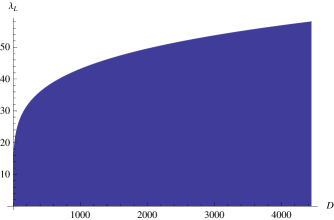
Figure 1: The value of the renormalized coupling $\tilde{\lambda}$ at the matching point as a function of the parameter $D$. The shaded area corresponds to the weak coupling regime of the theory.

The value of the renormalized coupling $\lambda_{*}$ at the matching point between the regimes (4.1), (4.2) and (4.13), (4.11) can be found from the matching condition for the beta function

$$D\lambda_{*}\approx\frac{3}{16\pi^{2}}\lambda_{*}^{2}-\frac{17}{768\pi^{4}}\lambda_{*}^{4}+\ldots,$$ (5.4)

where the l.h.s. of this equality represents the universal contribution to the beta function (4.13). After the substitution of the expression for the beta function up to 3 loops [29] into the r.h.s. of (5.4), we find $\lambda_{*}(D=2)\approx 12.66$ and $\lambda_{*}(D=4)\approx 14.53$. The first value corresponds to the situation when matching takes place at small momenta $\Lambda\ll\sqrt{2}H$, while the second to matching at $\Lambda\approx\sqrt{2}H$. Both values $\lambda_{*}$ are well below the tree level unitarity bound but above the region of validity of the 1-loop approximation for the beta function. Generally, the function $\lambda_{*}=\lambda_{*}(D)$ is a slowly changing function of the parameter $D$, finally reaching tree level unitarity bound around $D\approx{}4450$, see Fig. 1. Since the parameter $D$ determines the order of magnitude of the scaling violation corrections, we see that the strong coupling regime with $\lambda_{*}$ of the order of the tree level unitarity bound is realized when scaling violations are already very strong, confirming the main conclusion of [4]: a truly strongly coupled regime with $\lambda\geq\frac{32\pi}{\sqrt{3}}$ and negligible scaling violation cannot be achieved in $\lambda\phi^{4}_{4}$ theory.

Finally, we would like to point out that the formalism developed in Sections 2, 3 and 4 is perfectly applicable for the analysis of the high energy behavior of the $\lambda\phi^{4}$ theory in $d=2,3$ dimensions, where it leads to the scaling behavior

$$\beta(\tilde{\lambda})\approx d\tilde{\lambda}$$

in the transient regime. For $d=2$ the value of the beta function coincides with the exact result [30].

Acknowledgments

I would like to thank P.H. Damgaard, L. Motl and A. Polyakov for comments. E. Greenwood, T. Vachaspati and P. Vaudrevange have made numerous valuable suggestions thats helped to improve the text of the paper. This work is supported by grants from NASA and US DOE to the particle astrophysics theory group at CWRU.

References

- [1] K. G. Wilson and J. B. Kogut, Phys. Rept. 12, 75 (1974).
- [2] L.D. Landau, in “Niels Bohr and the development of physics”, ed. W. Pauli, Pergamon Press, 1955; L. D. Landau, A. Abrikosov and L. Khalatnikov, Nuovo Cim. Suppl. 3, 80 (1956).
- [3] M. A. B. Beg, C. Panagiotakopoulos and A. Sirlin, Phys. Rev. Lett. 52, 883 (1984); J. Kuti, L. Lin and Y. Shen, Phys. Rev. Lett. 61, 678 (1988); T. Hambye and K. Riesselmann, Phys. Rev. D 55, 7255 (1997) [arXiv:hep-ph/9610272].
- [4] M. Luscher and P. Weisz, Nucl. Phys. B 290, 25 (1987).
- [5] M. Aizenman, R. Graham, Nucl. Phys.B 225, 261 (1983); C. Aragao De Carvalho, S. Caracciolo and J. Frohlich, Nucl. Phys. B 215, 209 (1983).
- [6] I. T. Drummond, S. Duane and R. R. Horgan, Nucl. Phys. B 280, 25 (1987); J. Kuti and Y. Shen, Phys. Rev. Lett. 60, 85 (1988).
- [7] M. Aizenman, Phys. Rev. Lett. 47, 886 (1981).
- [8] M. Aizenman, Commun. Math. Phys. 86, 1 (1982).
- [9] G. Parisi and Y. s. Wu, Sci. Sin. 24, 483 (1981).
- [10] P. H. Damgaard and H. Huffel, Phys. Rept. 152, 227 (1987).
- [11] R. Dijkgraaf, D. Orlando and S. Reffert, Nucl. Phys. B 824, 365 (2010) [arXiv:0903.0732 [hep-th]].
- [12] A. Vilenkin, Phys. Lett. B 117, 25 (1982); J. B. Hartle and S. W. Hawking, Phys. Rev. D 28, 2960 (1983).
- [13] A brief review of the causal structure of de Sitter space can be found in M. Spradlin, A. Strominger and A. Volovich, in “Unity from duality: gravity, gauge theory and strings”, edited by C.P. Bachas, A. Bilal, M.R. Douglas, N.A. Nekrasov and F. David, p. 423 (Springer, 2003), arXiv:hep-th/0110007.
- [14] A. Starobinsky, in “Field theory, quantum gravity and strings”, edited by H.J. de Vega and N. Sanchez, (Springer-Verlag, 1986) p.107.
- [15] S. J. Rey, Nucl. Phys. B 284, 706 (1987); K. i. Nakao, Y. Nambu and M. Sasaki, Prog. Theor. Phys. 80 (1988) 1041; Y. Nambu and M. Sasaki, Phys. Lett. B 219, 240 (1989); D.S. Salopek and J.R. Bond, Phys. Rev. D 43, 1005 (1991); A.A. Starobinsky and J. Yokoyama, Phys. Rev. D 50 (1994) 6357 [arXiv:astro-ph/9407016].
- [16] P. M. Vaudrevange, D. I. Podolsky and G. D. Starkman, arXiv:0911.3397 [astro-ph.CO].
- [17] See A. H. Guth, Phys. Rept. 333, 555 (2000) [arXiv:astro-ph/0002156] for the review.
- [18] H. Nicolai, Phys. Lett. B 89, 341 (1980).
- [19] A. Strominger, JHEP 0111, 049 (2001) [arXiv:hep-th/0110087]; R. Bousso, A. Maloney and A. Strominger, Phys. Rev. D 65, 104039 (2002) [arXiv:hep-th/0112218].
- [20] A. Vilenkin, Nucl. Phys. B 226, 527 (1983).
- [21] A. M. Polyakov, Nucl. Phys. B 797, 199 (2008) [arXiv:0709.2899 [hep-th]]; A. M. Polyakov, arXiv:0912.5503 [hep-th].
- [22] A. Sokal, J. Stat. Phys. 28, 3 (1982); J. Zinn-Justin, “Quantum field theory and critical phenomena”, (Oxford University Press, 2003).
- [23] M. Namiki, “Stochastic quantization”, Chapter 8, Lecture Notes in Physics (Springer-Verlag, 1992).
- [24] J. Zinn-Justin, Nucl. Phys. B 275, 135 (1986); M. Namiki and Y. Yamanaka, Prog. Theor. Phys. 75, 1447 (1986).
- [25] K. Symanzik, in “Recent developments in gauge theories”, Eds. G. ’t Hooft et al., Plenum Press, New York, 1980; K. Symanzik, Nucl. Phys. B 226, 187 (1983).
- [26] See I. M. Suslov, arXiv:0804.0368 [hep-ph]. and references therein.
- [27] G. ’t Hooft, in “The Whys of Subnuclear Physics: Proceedings of the 1977 International School of Subnuclear Physics”, Ed. A. Zichichi (Plenum Press, New York, 1979).
- [28] I. M. Suslov, Zh. Eksp. Teor. Fiz. 116, 369 (1999) [J. Exp. Theor. Phys. 89, 197 (1999)] [arXiv:hep-ph/0002051].
- [29] D. I. Kazakov, O. V. Tarasov and A. A. Vladimirov, Sov. Phys. JETP 50, 521 (1979) [Zh. Eksp. Teor. Fiz. 77, 1035 (1979)].
- [30] G. Jug and B. N. Shalaev, J. Phys. A 32, 7249 (1999) [arXiv:cond-mat/9908068].