Universal scaling laws for dispersion interactions

Abstract

We study the scaling behaviour of dispersion potentials and forces under very general conditions. We prove that a rescaling of an arbitrary geometric arrangement by a factor $a$ changes the atom–atom and atom–body potentials in the long-distance limit by factors $1/a^{7}$ and $1/a^{4}$, respectively and the Casimir force per unit area by $1/a^{4}$. In the short-distance regime, electric and magnetic bodies lead to different scaling behaviours. As applications, we present scaling functions for two atom–body potentials and display the equipotential lines of a plate-assisted two-atom potential.

Scaling laws play a prominent role in the formulation of many physical problems and occur naturally when studying critical phenomena in particle physics, condensed matter and statistical mechanics. One example is percolation theory Aharony and Stauffer (1994), which has found applications in understanding forest fires, oil-field extraction and even measurement-based quantum computing Kieling et al. (2007).

Dispersion forces are effective quantum electromagnetic forces between neutral, but polarisable objects Milton (2004); Buhmann and Scheel (2007). Casimir and Polder found that dispersion forces are governed by simple power laws in the long-distance limit Casimir and Polder (1948): The potential of a ground-state atom at a distance $z_{A}$ from a perfectly conducting plate and that of two ground-state atoms separated by a distance $r_{AB}$ are proportional to $1/z_{A}^{4}$ and $1/r_{AB}^{7}$, respectively, while the force per unit area between two perfectly conducting plates at separation $z$ follows a $1/z^{4}$ law. Dispersion forces have since been studied for various bodies of simple shapes such as semi-infinite half spaces Henkel and Joulain (2005), plates of finite thickness Boström and Sernelius (2000); Buhmann et al. (2005), cylinders Mehl and Schaich (1980) and spheres Marvin and Toigo (1982); Taddei et al. (2009). In all of these cases, simple scaling laws have been found for the long- and short-distance limits.

For electrostatic or gravitational interactions, power laws for the forces between extended objects follow immediately by a volume integration of $1/r$ potentials. Dispersion forces, on the contrary, are due to an infinite hierarchy of microscopic $N$-point potentials Milonni and Lerner (1992), leading to a nontrivial geometry-dependence. Many-body effects and the nontrivial dependence on geometry are at the heart of current endeavours to gain a thorough theoretical Lambrecht and Marachevsky (2008) and experimental understanding Roy and Mohideen (1999) of the Casimir effect and to exploit it in nanotechnology applications Ashourvan et al. (2007a). The lack of simple analytical solutions for dispersion forces in complex scenarios necessitates general qualitative laws for what is achievable. Along these lines, it has been proven that mirror-symmetric arrangements always lead to attractive Casimir forces Kenneth and Klich (2006), and duality invariance has been established as a tool to study magnetoelectric effects Buhmann and Scheel (2009). Scaling laws of the kind observed for simple objects would be a powerful addition to this toolbox of general laws, provided that they can be formulated beyond the special cases mentioned above.

With this in mind, we will demonstrate in this Letter that for objects of arbitrary shapes, dispersion interactions in the long- and short-distance limits obey scaling laws; and we will identify the respective scaling powers. Our proof relies on the known dependence of dispersion potentials on the atomic polarisability $\alpha(\omega)$, body permittivity $\varepsilon(\bm{r},\omega)$ and permeability $\mu(\bm{r},\omega)$, where the latter determines the electromagnetic Green tensor

$$\biggl{[}\bm{\nabla}\!\times\!\frac{1}{\mu(\bm{r},\omega)}\bm{\nabla}\!\times\!\,-\,\frac{\omega^{2}}{c^{2}}\,\varepsilon(\bm{r},\omega)\biggr{]}\mbox{{{{G}}}}(\bm{r},\bm{r}^{\prime},\omega)=\bm{\delta}(\bm{r}-\bm{r}^{\prime}).$$ (1)

In terms of these quantities, the Casimir–Polder (CP) potential of a single electric ground-state atom and the van der Waals (vdW) potential of two such atoms read

$$U(\bm{r}_{A})=\frac{\hbar\mu_{0}}{2\pi}\int_{0}^{\infty}\mathrm{d}\xi\,\xi^{2}\alpha_{A}(\mathrm{i}\xi)\operatorname{Tr}\mbox{{{{G}}}}^{(1)}(\bm{r}_{A},\bm{r}_{A},\mathrm{i}\xi),$$ (2)

($\mbox{{{{G}}}}=\mbox{{{{G}}}}^{(0)}+\mbox{{{{G}}}}^{(1)}$; bulk and scattering parts) and

$$U(\bm{r}_{A},\bm{r}_{B})=-\frac{\hbar\mu_{0}^{2}}{2\pi}\int_{0}^{\infty}\mathrm{d}\xi\,\xi^{4}\alpha_{A}(\mathrm{i}\xi)\alpha_{B}(\mathrm{i}\xi)\\[2.15277pt] \times\operatorname{Tr}[\mbox{{{{G}}}}(\bm{r}_{A},\bm{r}_{B},\mathrm{i}\xi)\!\cdot\!\mbox{{{{G}}}}(\bm{r}_{B},\bm{r}_{A},\mathrm{i}\xi)],$$ (3)

respectively, and the Casimir force on a body of volume $V$ is given by $\bm{F}=\int_{\partial V}\mathrm{d}\bm{A}\!\cdot\!\mbox{{{{T}}}}(\bm{r})$ with

$$\mbox{{{{T}}}}(\bm{r})=-\frac{\hbar}{\pi}\int_{0}^{\infty}\mathrm{d}\xi\biggl{\{}\biggl{[}\frac{\xi^{2}}{c^{2}}\,\mbox{{{{G}}}}^{(1)}(\bm{r},\bm{r},\mathrm{i}\xi)\\ +\bm{\nabla}\!\times\!\mbox{{{{G}}}}^{(1)}(\bm{r},\bm{r},\mathrm{i}\xi)\!\times\!\overleftarrow{\bm{\nabla}}^{\prime}\biggr{]}-\frac{1}{2}\operatorname{Tr}\biggl{[}\frac{\xi^{2}}{c^{2}}\,\mbox{{{{G}}}}^{(1)}(\bm{r},\bm{r},\mathrm{i}\xi)\\ +\bm{\nabla}\!\times\!\mbox{{{{G}}}}^{(1)}(\bm{r},\bm{r},\mathrm{i}\xi)\!\times\!\overleftarrow{\bm{\nabla}}^{\prime}\biggr{]}\mbox{{{{I}}}}\biggr{\}}$$ (4)

(I: unit tensor) Buhmann and Scheel (2007). We will first define the general scaling problem and then solve it separately in the long- and short-distance cases.

The scaling problem.

Consider an arbitrary arrangement of linearly responding bodies characterised by their permittivity $\varepsilon(\bm{r},\omega)$ and permeability $\mu(\bm{r},\omega)$, with one or two atoms at positions $\bm{r}_{A}$ and $\bm{r}_{B}$ [Fig. 1(i)]. The scaled arrangement (scaling factor $a\neq 0$) is described by the permittivity and permeability

$$\overline{\varepsilon}(\bm{r},\omega)=\varepsilon(\bm{r}/a,\omega),\qquad\overline{\mu}(\bm{r},\omega)=\mu(\bm{r}/a,\omega);$$ (5)

with the atomic positions being scaled accordingly: $\overline{\bm{r}}_{A}=a\bm{r}_{A}$, $\overline{\bm{r}}_{B}=a\bm{r}_{B}$ [Fig. 1(ii)].

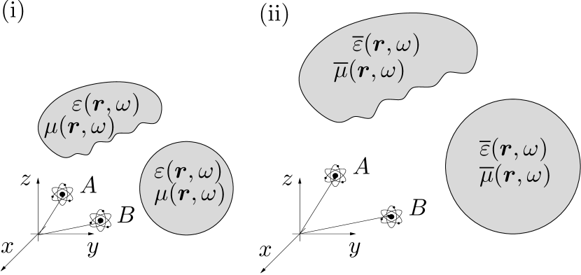
Figure 1: (i) Original and (ii) scaled configurations of bodies and atoms ($a=1.4$).

Interactions for long distances.

We speak of the long-distance regime when all distances are much larger than the wavelengths of the atomic and medium response functions. In this case, we can approximate the latter by their static values, $\alpha(\omega)\simeq\alpha$, $\varepsilon(\bm{r},\omega)\simeq\varepsilon(\bm{r})$, $\mu(\bm{r},\omega)\simeq\mu(\bm{r})$, so the Green tensor is determined by

$$\biggl{[}\bm{\nabla}\!\times\!\frac{1}{\mu(\bm{r})}\bm{\nabla}\!\times\!\,-\,\frac{\omega^{2}}{c^{2}}\,\varepsilon(\bm{r})\biggr{]}\mbox{{{{G}}}}(\bm{r},\bm{r}^{\prime},\omega)=\bm{\delta}(\bm{r}-\bm{r}^{\prime}).$$ (6)

The Green tensor of the scaled arrangement obeys

$$\biggl{[}\bm{\nabla}\!\times\!\frac{1}{\overline{\mu}(\bm{r})}\bm{\nabla}\!\times\!\,-\,\frac{\omega^{2}}{c^{2}}\,\overline{\varepsilon}(\bm{r})\biggr{]}\overline{\mbox{{{{G}}}}}(\bm{r},\bm{r}^{\prime},\omega)=\bm{\delta}(\bm{r}-\bm{r}^{\prime}).$$ (7)

By renaming $\bm{r}\mapsto a\bm{r}$, $\omega\mapsto\omega/a$ and using Eq. (5) and $\delta(a\bm{r})=\delta(\bm{r})/a^{3}$, we find that

$$\biggl{[}\bm{\nabla}\!\times\!\frac{1}{\mu(\bm{r})}\bm{\nabla}\!\times\!\,-\,\frac{\omega^{2}}{c^{2}}\,\varepsilon(\bm{r})\biggr{]}a\overline{\mbox{{{{G}}}}}(a\bm{r},a\bm{r}^{\prime},\omega/a)=\bm{\delta}(\bm{r}-\bm{r}^{\prime}).$$ (8)

Comparison with Eq. (6) reveals the scaling

$$\overline{\mbox{{{{G}}}}}(a\bm{r},a\bm{r}^{\prime},\omega/a)=(1/a)\mbox{{{{G}}}}(\bm{r},\bm{r}^{\prime},\omega).$$ (9)

Substitution into the CP potential (2) leads to

$$\overline{U}(a\bm{r}_{A})=\frac{\hbar\mu_{0}\alpha_{A}}{2\pi}\int_{0}^{\infty}\mathrm{d}\xi\,\xi^{2}\,\operatorname{Tr}\overline{\mbox{{{{G}}}}}^{(1)}(a\bm{r}_{A},a\bm{r}_{A},\mathrm{i}\xi)\\ =\frac{\hbar\mu_{0}\alpha_{A}}{2\pi}\int_{0}^{\infty}\frac{\mathrm{d}\xi}{a}\,\frac{\xi^{2}}{a^{2}}\,\,\operatorname{Tr}\overline{\mbox{{{{G}}}}}^{(1)}(a\bm{r}_{A},a\bm{r}_{A},\mathrm{i}\xi/a)\\ =(1/a^{4})U(\bm{r}_{A}).$$ (10)

The CP force thus scales as $\overline{\bm{F}}(a\bm{r}_{A})=(1/a^{5})\bm{F}(\bm{r}_{A})$. Analogously, Eq. (9) can be used to derive the following scaling laws for the vdW potential (3) and the Casimir force per unit area (4):

$$\overline{U}(a\bm{r}_{A},a\bm{r}_{B})=(1/a^{7})U(\bm{r}_{A},\bm{r}_{B}),$$ (11)

$$\overline{\mbox{{{{T}}}}}(a\bm{r})=(1/a^{4})\mbox{{{{T}}}}(\bm{r}),$$ (12)

so the total Casimir force behaves as $\overline{\bm{F}}=(1/a^{2})\bm{F}$.

Interactions for short distances.

In the short-distance or nonretarded regime, all distances are much smaller than the characteristic atomic and medium wavelengths. A simple example shows that here no universal scaling law exists in the general case: The nonretarded CP potential of an atom at distance $z_{A}$ from a magnetoelectric half space reads Buhmann et al. (2005)

$$U(z_{A})=-\frac{C_{3}}{z_{A}^{3}}+\frac{C_{1}}{z_{A}},$$ (13)

which is incompatible with a relation of the form (10).

However, scaling laws can still be formulated by distinguishing between purely electric and purely magnetic environments. For purely electric bodies, the Green tensor (1) can be given by the Dyson equation Buhmann and Scheel (2007)

$$\mbox{{{{G}}}}(\bm{r},\bm{r}^{\prime},\omega)=\mbox{{{{G}}}}^{(0)}(\bm{r},\bm{r}^{\prime},\omega)\\ +\frac{\omega^{2}}{c^{2}}\int\mathrm{d}^{3}s\,\chi(\bm{s},\omega)\mbox{{{{G}}}}^{(0)}(\bm{r},\bm{s},\omega)\!\cdot\!\mbox{{{{G}}}}(\bm{s},\bm{r}^{\prime},\omega)$$ (14)

($\chi=\varepsilon-1$) where

$$\mbox{{{{G}}}}^{(0)}(\bm{r},\bm{r}^{\prime},\omega)=-\frac{c^{2}\mathrm{e}^{\mathrm{i}\omega\rho/c}}{4\pi\omega^{2}\rho^{3}}\biggl{\{}\biggl{[}1-\mathrm{i}\,\frac{\omega\rho}{c}-\Bigl{(}\frac{\omega\rho}{c}\Bigr{)}^{2}\biggr{]}\mbox{{{{I}}}}\\ -\biggl{[}3-3\mathrm{i}\,\frac{\omega\rho}{c}-\Bigl{(}\frac{\omega\rho}{c}\Bigr{)}^{2}\biggr{]}\bm{e}_{\rho}\bm{e}_{\rho}\biggr{\}}-\frac{c^{2}}{3\omega^{2}}\,\bm{\delta}(\bm{\rho})$$ (15)

($\bm{\rho}=\bm{r}-\bm{r}^{\prime}$) is the free-space Green tensor. In the short-distance limit $\omega\rho/c\ll 1$, the latter reduces to

$$\mbox{{{{G}}}}^{(0)}(\bm{r},\bm{r}^{\prime},\omega)=-\frac{c^{2}[\mbox{{{{I}}}}-3\bm{e}_{\rho}\bm{e}_{\rho}]}{4\pi\omega^{2}\rho^{3}}-\frac{c^{2}}{3\omega^{2}}\,\bm{\delta}(\bm{\rho}).$$ (16)

Starting from the analogous Dyson equation for the scaled Green tensor, we make the substitutions $\bm{r}\mapsto a\bm{r}$, $\bm{r}^{\prime}\mapsto a\bm{r}^{\prime}$ and $\bm{s}\mapsto a\bm{s}$. After using Eq. (5) and the scaling $\mbox{{{{G}}}}^{(0)}(a\bm{r},a\bm{r}^{\prime},\omega)=(1/a^{3})\mbox{{{{G}}}}^{(0)}(\bm{r},\bm{r}^{\prime},\omega)$ of Eq. (16), a comparison with (14) reveals the scaling

$$\overline{\mbox{{{{G}}}}}(a\bm{r},a\bm{r}^{\prime},\omega)=(1/a^{3})\mbox{{{{G}}}}(\bm{r},\bm{r}^{\prime},\omega)$$ (17)

for the full Green tensor. Substitution into Eqs. (2)–(4) immediately implies the scaling laws

$$\overline{U}(a\bm{r}_{A})=(1/a^{3})U(\bm{r}_{A}),$$ (18)

$$\overline{U}(a\bm{r}_{A},a\bm{r}_{B})=(1/a^{6})U(\bm{r}_{A},\bm{r}_{B}),$$ (19)

$$\overline{\mbox{{{{T}}}}}(a\bm{r})=(1/a^{3})\mbox{{{{T}}}}(\bm{r})$$ (20)

where we have used the fact that $\mbox{{{{G}}}}^{(1)}$ dominates over $\bm{\nabla}\!\times\!\mbox{{{{G}}}}^{(1)}\!\times\!\overleftarrow{\bm{\nabla}}^{\prime}$ in the short-distance limit.

For an arrangement of purely magnetic bodies, the nonretarded Green tensor obeys the Dyson equation

$$\mbox{{{{G}}}}^{(1)}(\bm{r},\bm{r}^{\prime},\omega)=\int\mathrm{d}^{3}s\,\zeta(\bm{s},\omega)\bigl{[}\mbox{{{{G}}}}^{(0)}(\bm{r},\bm{s},\omega)\!\times\!\overleftarrow{\bm{\nabla}}_{\!\bm{s}}\bigr{]}\\ \!\cdot\!\bigl{[}\bm{\nabla}_{\!\bm{s}}\!\times\!\mbox{{{{G}}}}^{(0)}(\bm{s},\bm{r}^{\prime},\omega)+\bm{\nabla}_{\!\bm{s}}\!\times\!\mbox{{{{G}}}}^{(1)}(\bm{s},\bm{r}^{\prime},\omega)\bigr{]}$$ (21)

($\zeta=1/\mu-1$) with nonretarded free-space Green tensors

$$\bm{\nabla}\!\times\!\mbox{{{{G}}}}^{(0)}(\bm{r},\bm{r}^{\prime},\omega)=-\mbox{{{{G}}}}^{(0)}(\bm{r},\bm{r}^{\prime},\omega)\!\times\!\overleftarrow{\bm{\nabla}}^{\prime}=-\frac{\bm{e}_{\rho}\!\times\!\mbox{{{{I}}}}}{4\pi\rho^{2}}\,.$$ (22)

We read off $(1/a^{2})$ scalings for $\bm{\nabla}\!\times\!\mbox{{{{G}}}}^{(0)}$ and $\mbox{{{{G}}}}^{(0)}\!\times\!\overleftarrow{\bm{\nabla}}^{\prime}$, so following similar steps as above, the Dyson equation (21) together with Eq. (5) implies

$$\overline{\mbox{{{{G}}}}}{}^{(1)}(a\bm{r},a\bm{r}^{\prime},\omega)=(1/a)\mbox{{{{G}}}}^{(1)}(\bm{r},\bm{r}^{\prime},\omega).$$ (23)

Using Eq. (2), the nonretarded CP potential scales as

$$\overline{U}(a\bm{r}_{A})=(1/a)U(\bm{r}_{A})$$ (24)

for purely magnetic bodies. The vdW potential (3) contains contributions from the bulk and scattering Green tensors with different scalings. We separate it into a free-space part $U^{(0)}$ that contains only $\mbox{{{{G}}}}^{(0)}$ and scales according to Eq. (19) and a body-induced part $U^{(1)}$. The latter is dominated by the mixed terms $\mbox{{{{G}}}}^{(0)}\mbox{{{{G}}}}^{(1)}$ for purely magnetic bodies in the short-distance limit; it scales as

$$\overline{U}{}^{(1)}(a\bm{r}_{A},a\bm{r}_{B})=(1/a^{4})U^{(1)}(\bm{r}_{A},\bm{r}_{B}).$$ (25)

The Casimir force (4) is dominated by $\bm{\nabla}\!\times\!\mbox{{{{G}}}}^{(1)}\!\times\!\overleftarrow{\bm{\nabla}}^{\prime}$ with its $(1/a^{3})$ scaling for purely magnetic bodies, so that

$$\overline{\mbox{{{{T}}}}}(a\bm{r})=(1/a^{3})\mbox{{{{T}}}}(\bm{r}).$$ (26)

Figure 2: Scale functions for the potential of an atom in front of a Si plate (solid line) and near a perfectly conducting sphere (dashed line).

Applications.

In the simplest situations where dispersion forces depend on a single distance parameter, the scaling laws directly determine the dependence on that parameter. For instance, the long-distance scaling laws (10)–(12) imply the power laws for dispersion interactions involving atoms and perfectly conducting plates mentioned above.

For a class of geometries involving a distance parameter $z$ and a single size parameter $d$, the scaling laws can be employed to write potentials and forces in the form $(C_{k}/z^{k})f(d/z)$, all relevant information being contained in the scaling function $f(x)$. In Fig. 2 we display the scaling functions for the potential of an atom at distance $z_{A}$ from a Si plate of thickness $d$ ($x=d/z_{A}$) in the long-distance limit Buhmann et al. (2005) and for the nonretarded potential of a perfectly conducting sphere of radius $R$ ($x=R/z_{A}$) Taddei et al. (2009).

The plate potential reaches its half-plate limit with associated $1/z_{A}^{4}$ asymptote already for $x=d/z_{A}\gtrsim 0.5$, showing that finite thickness effects can be neglected for moderately thick plates even for dielectrics. For very thin plates with $x=d/z_{A}\lesssim 0.1$, the scale function of the plate is linear for small $x$, implying a $x/z_{A}^{4}\propto 1/z_{A}^{5}$ potential. A rather abrupt change between the two power laws occurs between the two extremes.

The scale function of the sphere saturates much more slowly to its large-$x$ asymptote where a $1/z_{A}^{3}$ half-space potential is observed. This indicates that proximity force approximations Bloccki et al. (1977) should be used with care. The scale function of the sphere potential is cubic for small $x$, corresponding to a $x^{3}/z_{A}^{3}\propto 1/z_{A}^{6}$ asymptote.

As a more complex example, we consider the vdW potential of two atoms $A$ and $B$ in front of a perfectly conducting plate in the long-distance limit Spagnolo et al. (2006). In Fig. 3(i), we show the plate-induced enhancement of the potential with respect to its free space value for a given distance of atom $B$ from the plate. The results for a different distance can then be obtained from a scaling transformation, cf. Fig. 3(ii).

Figure 3: Retarded vdW potential next to a perfectly conducting plate. Atom $B$ is held at different fixed positions (large dot). The thick contour denotes $U/U^{(0)}=1$, values are increasing towards the exterior of this contour in steps of $0.02$.

The plate is seen to enhance the interatomic interaction in two lobe-shaped regions to the left and right of atom $B$. This implies that for a thin slab of an atomic gas at distance $z$ from the plate, the atom–atom correlation function will be enhanced at interatomic distances $r\simeq 2.5z$ corresponding to the centres of the lobes. By virtue of scale invariance, this holds for all $z$ that are compatible with the long-distance limit.

Summary and perspective.

By considering the scaling behaviour for the respective Green tensors, we have derived universal scaling laws for dispersion interactions in the long- and short-distance limits as summarised in Tab. 1.

Distance	Long	Short
Bodies	Magnetoelectric	Electric	Magnetic
$U(\bm{r}_{A})$	$1/a^{4}$	$1/a^{3}$	$1/a$
$U^{(0)}(\bm{r}_{A},\bm{r}_{B})$	$1/a^{7}$	$1/a^{6}$	$1/a^{6}$
$U^{(1)}(\bm{r}_{A},\bm{r}_{B})$	$1/a^{7}$	$1/a^{6}$	$1/a^{4}$
$\mbox{{{{T}}}}(\bm{r})$	$1/a^{4}$	$1/a^{3}$	$1/a^{3}$

Table 1: Scaling laws for the CP potential, free-space and body-induced vdW potentials and the Casimir pressure.

Scaling laws indicate the absence of a characteristic length scale of the system. For dispersion potentials, the typical interatomic distances and the wavelengths of atomic and body response functions give two such characteristic length scales. The nonretarded scaling laws are hence only valid for distances well between these two length scales while the long-range one is restricted to distances well above the latter.

The scaling laws may be used to deduce the functional dependence of dispersion forces in the case where they depend on only a single parameter. In more complex cases, the knowledge of a potential for a body of given size can be used the infer the potential for a similar body of different size. In particular, equipotential lines are invariant under a scale transformation. More complex applications include bodies with surface roughness. The duality invariance of dispersion forces Buhmann and Scheel (2009) can be used to extend our results to magnetic atoms.