Studying freeze-out and hadronization in the Landau hydrodynamical model

Abstract

We study the rapidity spectra in ultra-relativistic heavy ion collisions in the framework of the Landau hydrodynamical model. We find that thermal smearing effects improve the agreement with experimental results on pion rapidity spectra. We describe a simple model of the hadronization and discuss its consequences regarding the pion multiplicity and the increasing entropy condition.

I Introduction

The Landau hydrodynamical model Landau ; Landau2 is a simple approximate solution of the hydrodynamical equations describing the expansion of a thin disk of static gas. The original idea was to use hydrodynamics to describe collisions of very high energy hadrons, when a large number of new particles are created. Today the model is also frequently applied to the expansion of the Quark Gluon Plasma (QGP) formed in ultra-relativistic heavy ion collisions. It provides a good description of the shape of the rapidity distribution of pions Wong .

II Review of the Landau model

The initial state of the Landau hydrodynamical model is a thin static disk of thickness $\Delta$ and diameter $a$. It is assumed to be the approximation of the overlap of two highly Lorentz contracted nuclei, and the two geometrical sizes are assumed to be related by

$$\Delta=a/\gamma,$$ (1)

with $\gamma$ the Lorentz factor corresponding to the velocity of the colliding nuclei in the center-of-mass frame,

$$\gamma=\frac{\sqrt{S_{NN}}}{2m_{N}},$$ (2)

where $S_{NN}$ is the invariant collision energy per colliding nucleons of mass $m_{N}$.

The hydrodynamical evolution of the system is divided in two parts: the initial longitudinal expansion (during which transverse velocities and displacements are neglected), and the subsequent “conic flight”, where transverse velocities appear.

Assuming a simple equation of state (EOS) of the form

$$P=\epsilon/3,$$ (3)

an approximate solution of the 1+1 dimensional problem of the longitudinal expansion phase is given by Landau Landau . This solution is summarized (using the notation of Wong ) as follows. The energy-density field is

$$\epsilon(y_{+},y_{-})=\epsilon_{0}\exp\left\{-\frac{4}{3}\left(y_{+}+y_{-}-\sqrt{y_{+}y_{-}}\right)\right\},$$ (4)

where $y_{\pm}$ are logarithmic light-cone coordinates

$$y_{\pm}=\ln\frac{t\pm z}{\Delta},$$ (5)

and $\epsilon_{0}$ is the initial energy-density of the disk. The rapidity field is

$$y(t,z)=\frac{1}{2}\ln\frac{t+z}{t-z}\equiv\frac{1}{2}(y_{+}-y_{-}).$$ (6)

In the longitudinal expansion components of the flow four-velocity are expressed in terms of the flow rapidity as

$$u^{\mu}=(\cosh{y},0,0,\sinh{y})=\cosh{y}(1,0,0,v_{z})$$ (7)

which can be inverted to give

$$y=\frac{1}{2}\ln\frac{u^{0}+u^{3}}{u^{0}-u^{3}}=\tanh^{-1}{v_{z}}.$$ (8)

Looking at (6) one observes that the flow rapidity and the space-time rapidity coordinate coincide (the first expression in (6) is exactly the definition of space-time rapidity), similarly to the case of the Bjorken model. Because of the coincidence of flow rapidity and space-time rapidity the space-time coordinates of a fluid element and the components of its four-velocity are related by

$$u^{0}=\frac{t}{\tau},\qquad u^{3}=\frac{z}{\tau},$$ (9)

where we have introduced the proper time coordinate $\tau=\sqrt{t^{2}-z^{2}}$.

In Refs. Landau ; Wong an estimate of the transverse displacement of the system is given as

$$r(t,y)=\frac{t^{2}}{4a\cosh^{2}y}.$$ (10)

The transition to the second phase of “conic flight” is assumed to happen when this transverse displacement reaches the transverse size of the system, $a$. Using the relations Eq. (9) the condition of transition to conic flight can be written as

$$\tau_{\text{TR}}=2a.$$ (11)

This defines a hypersurface in space-time, which we call the transition hypersurface.

Although Landau ; Wong give a sketch of the hydrodynamical evolution of the system in the second phase of conic flight, in the calculation of observables they assume that freeze-out happens immediately, i.e. not only the flight angle $\theta$ of fluid elements is assumed to be frozen on the transition hypersurface defined by Eq. (11), but also the fluid is replaced by an ensemble of non-interacting particles traveling with the same constant velocity. Thus, the transition hypersurface is also the freeze-out (FO) hypersurface (and the subscripts TR and FO can be interchanged). The velocity of particles is assumed to coincide with the velocity of the fluid element at the FO hypersurface, which means that no smearing effect coming from the thermal distribution of particles in the fluid is taken into account.

Equation (11) gives a relation between the time of freeze-out and the position of the fluid element at freeze-out of the form

$$t_{\text{FO}}(z)\equiv t_{\text{TR}}(z)=\sqrt{4a^{2}+z^{2}}.$$ (12)

This means that at the freeze-out the system can be described in terms of functions of one variable, say $z_{\text{FO}}$. (Because of azimuthal symmetry everything is independent of the azimuth angle $\phi$, furthermore, everything is assumed to be independent of the radial coordinate $r$ for $r<a$, and to vanish for $r>a$). Furthermore, there is a one-to-one correspondence between $z$ and the fluid rapidity $y$ on the FO hypersurface of the form (see Eqs. (7), (9) and (11))

$$z_{\text{FO}}=2a\sinh{y},$$ (13)

so instead of $z_{\text{FO}}$ we can use $y$ as the independent variable. Using Eq. (12) the FO time can be expressed in terms of $y$ as

$$t_{FO}=2a\cosh{y}.$$ (14)

In order to get the rapidity distribution of particles we start from the expression of the total particle number

$$N=\int N^{\mu}d\sigma_{\mu},$$ (15)

with $N^{\mu}=nu^{\mu}$ the particle current ($n$ is the invariant scalar particle density), and $d\sigma_{\mu}$ the hypersurface element four-vector. Using cylindrical coordinates $(r,\phi,z)$ the FO hypersurface is given by

$$x^{\mu}(r,\phi,z)=\left(t_{\text{FO}}(z),r\cos\phi,r\sin\phi,z\right)$$ (16)

and so

$$d\sigma_{\mu}=\epsilon_{\mu\nu\rho\sigma}\partial_{r}x^{\nu}\partial_{\phi}x^{\rho}\partial_{z}x^{\sigma}drd\phi dz=\left(1,0,0,-\partial_{z}t_{\text{FO}}(z)\right)rdrd\phi dz.$$ (17)

From Eq. (12)

$$\partial_{z}t_{\text{FO}}(z)=\tanh{y},$$ (18)

and changing the integration variable $z$ to $y$ gives

$$dz=2a\cosh{y}dy.$$ (19)

The $\phi$ and $r$ integrations give a factor

$$\int_{0}^{2\pi}d\phi\int_{0}^{a/2}rdr\rightarrow\frac{a^{2}\pi}{4},$$ (20)

so finally

$$d\sigma_{\mu}\rightarrow\frac{a^{3}\pi}{2}\left(\cosh{y},0,0,-\sinh{y}\right)dy.$$ (21)

We now assume that the transverse component of the velocity is negligible, so $u^{0}$ and $u^{3}$ are given by (7) at FO too. Therefore

$$u^{\mu}d\sigma_{\mu}\rightarrow\frac{a^{3}\pi}{2}dy.$$ (22)

We assume that QGP is an ensemble of massless quarks and gluons, and obeys the Stefan-Boltzmann EOS, $\epsilon\propto T^{4}$ (which is consistent with (3)). In that case

$$n\propto T^{3}\propto\epsilon^{3/4}=\epsilon_{0}^{3/4}\exp\left\{-\left(y_{+}+y_{-}-\sqrt{y_{+}y_{-}}\right)\right\},$$ (23)

where we have used Eq. (4) in the last step. As described in Wong , from Eq. (5) it follows that on the FO surface $y_{\pm}|_{\text{FO}}=y_{b}\pm y$, where $y_{b}=\ln(2a/\Delta)=\ln(\sqrt{s_{NN}}/m_{N})$ is the rapidity of the colliding nuclei in the CM frame. Therefore the exponent in (23) can be written on the FO surface as $\left(y_{+}+y_{-}-\sqrt{y_{+}y_{-}}\right)|_{\text{FO}}=2y_{b}-\sqrt{y_{b}^{2}-y^{2}}$. Using this in (23) we get the invariant particle number density on the FO hypersurface expressed as a function of $y$:

$$n(y)\propto\exp\left\{\sqrt{y_{b}^{2}-y^{2}}\right\}.$$ (24)

The rapidity distribution of particles, $dN/dy$ is obtained by differentiating (15). Thus, making use of (22) and (24) we get

$$dN/dy\propto\exp\left\{\sqrt{y_{b}^{2}-y^{2}}\right\},$$ (25)

in agreement with Wong .

III Thermal effects

The starting point of the calculation of observables is the momentum distribution of emitted particles, which develops at freeze-out. In the case of sudden FO happening on a hypersurface the invariant momentum distribution is given by the Cooper-Frye formula Cooper_Frye

$$E\frac{d^{3}N}{d\mathbf{p}^{3}}=\int f(x,p)p^{\mu}d\sigma_{\mu},$$ (26)

where $f(x,p)$ is the phase-space distribution of particles after freeze-out.

In hydrodynamics local thermal equilibrium is assumed, therefore the $x$ dependence of $f$ is encoded in the space-time dependence of the parameters of the thermal distributions, $T(x)$ and $u^{\mu}(x)$. (The Stefan-Boltzmann EOS $\epsilon\propto T^{4}$ restricts the considerations to baryonfree media, therefore the baryo-chemical potential is zero.) The thermal phase-space distribution has the general form

$$f(x,p)=\tilde{f}\left(\frac{p^{\mu}u_{\mu}(x)}{T(x)}\right)=\frac{g}{(2\pi)^{3}}\frac{1}{\exp\left(\frac{p^{\mu}u_{\mu}(x)}{T(x)}\right)+\xi},$$ (27)

with $\xi$=1 for fermions, -1 for bosons and 0 for classical particles obeying Boltzmann statistics. $g$ is a degeneracy factor that is different for each particle species.

In the case of the Landau model parameters of the fluid taken on the FO hypersurface depend on only one variable, which can be chosen the fluid rapidity $y$. The expression for $T(y)$ can be obtained from the expression of the energy density, Eq. (4), assuming the Stefan-Boltzmann EOS $\epsilon=\sigma T^{4}$. Following the steps leading to the expression (25) we get the result

$$T(y)=\left(\frac{\epsilon_{0}}{\sigma}\right)^{1/4}e^{-2y_{b}/3}\exp\left\{\frac{1}{3}\sqrt{y_{b}^{2}-y^{2}}\right\}.$$ (28)

The transverse velocity of fluid elements is assumed to be negligible at FO. Components of the four-velocity of the fluid are given (in accordance with (7)) by

$$u^{\mu}(y)=(\cosh{y},0,0,\sinh{y}).$$ (29)

A comment concerning the validity of the model is appropriate here. Because of the relation $u^{\mu}u_{\mu}=1$ the inclusion of a nonzero transverse velocity of the fluid would require the modification of Eq. (7). But the relations (7) are a key ingredient of the Landau model related to the separation of longitudinal and transverse expansion of the system. Their modification would destroy the simplicity of the model.

An estimate of the transverse velocity of fluid elements can be obtained by differentiating (10). We get

$$v_{r}=\frac{dr(t,y)}{dt}=\frac{t}{2a\cosh^{2}y}.$$ (30)

Using Eq. (14) this gives

$$v_{r}|_{\text{FO}}=\frac{1}{\cosh{y}}$$ (31)

on the FO hypersurface. On the other hand Eq. (7) gives $v_{z}=u^{3}/u^{0}=\tanh{y}$ for the longitudinal velocity component, which implies

$$v^{2}=v_{r}^{2}+v_{z}^{2}=1,$$ (32)

meaning that fluid elements would reach the speed if light at FO if one included a transverse velocity with the above approximations. This also indicates that the Landau model — although it gives a good description of rapidity spectra — is not a suitable model for describing e.g. the transverse momentum distribution of particles, at least not in its simplest form.

The four-momentum of particles can be specified as

$$p^{\mu}=(m_{T}\cosh{y_{p}},p_{T}\cos{\phi_{p}},p_{T}\sin{\phi_{p}},m_{T}\sinh{y_{p}})$$ (33)

in terms of their transverse momentum $p_{T}$, rapidity $y_{p}$ and azimuth angle $\phi_{p}$, where $m_{T}=\sqrt{m^{2}+p_{T}^{2}}$ is the transverse mass, with the mass of the particle, $m$. From Eqs. (29) and (33)

$$p^{\mu}u_{\mu}(x)=m_{T}\cosh(y-y_{p}).$$ (34)

In order to calculate the rapidity distribution of emitted particles one first has to express the invariant momentum distribution, Eq. (26) in variables $p_{T}$, $y_{p}$ and $\phi_{p}$,

$$E\frac{d^{3}N}{d\mathbf{p}^{3}}=\frac{d^{3}N}{p_{T}dp_{T}dy_{p}d\phi_{p}}.$$ (35)

Integrating this, and substituting the right hand side of (26) we get for the rapidity spectrum

$$\frac{dN}{dy_{p}}=\int dp_{T}p_{T}d\phi_{p}E\frac{d^{3}N}{d\mathbf{p}^{3}}=\int dp_{T}p_{T}d\phi_{p}\int f(x,p)p^{\mu}d\sigma_{\mu}.$$ (36)

Here $d\sigma^{\mu}$ is given by (17). The integrand is independent of the azimuth angles $\phi$ and $\phi_{p}$ corresponding to the position of the fluid element and the particle momentum, and the radial coordinate $r$ (see Eqs. (27), (28) and (34)). This means that the effect of the $d\sigma^{\mu}$ integration is the same as given by (21) and the integral over $\phi_{p}$ yields a factor of $2\pi$. The rapidity distribution is then (also making the change of integration variable $p_{T}\rightarrow m_{T}$)

$$\frac{dN}{dy_{p}}=a^{3}\pi^{2}\int\limits_{m}^{\infty}dm_{T}m_{T}^{2}\int\limits_{-\infty}^{\infty}dy\cosh(y-y_{p})\tilde{f}\left(\frac{p^{\mu}u_{\mu}(y)}{T(y)}\right).$$ (37)

IV The hadronization phase transition

In accordance with the Stefan-Boltzmann EOS assumed in the Landau model the expanding quark-gluon plasma (QGP) is assumed to be an ensemble of massless quarks, antiquarks and gluons. The EOS also requires that the QGP is baryonfree, which is a reasonable approximation at RHIC or LHC energies, where the particle spectra are dominated by secondaries.

On the other hand, the post freeze-out (PFO) hadronic medium is an ensemble of massive particles of different species. We assume that the phase transition from QGP to hadronic matter happens at the FO hypersurface (simultaneous FO and hadronization). Physical parameters of the two media are related via the prescription of boundary conditions on the FO hypersurface describing energy and momentum conservation,

$$\left[T^{\mu\nu}d\hat{\sigma}_{\nu}\right]=0,$$ (38)

where the meaning of the square bracket is $[a]=a|_{\text{PFO}}-a|_{\text{QGP}}$. The energy-momentum tensor has the form

$$T^{\mu\nu}=(\epsilon+P)u^{\mu}u^{\nu}-Pg^{\mu\nu}$$ (39)

in ideal hydrodynamics. $d\hat{\sigma}_{\mu}$ is unit four-vector normal to the FO hypersurface. In the Landau model this is given by

$$d\hat{\sigma}_{\mu}=d{\sigma}_{\mu}/\sqrt{d{\sigma}^{\rho}d{\sigma}_{\rho}}=(\cosh{y},0,0,-\sinh{y})\equiv u_{\mu}$$ (40)

(see (21) and (29)). The last equation reflects a general property of the Landau model, namely, that the four-velocity of the fluid is everywhere normal to hypersurfaces characterized by a constant space-time rapidity $\tau$, in particular to our FO hypersurface. This feature of the Landau model is the same as in the Bjorken model. Making use of relation (40) the condition of energy-momentum conservation Eq. (38) becomes

$$\left[\epsilon u^{\mu}\right]=0.$$ (41)

The component of (41) parallel to $d\hat{\sigma}_{\mu}$ tells us that the invariant energy density is constant across the FO hypersurface, $[\epsilon]=0$, while the disappearance of the component normal to $d\hat{\sigma}_{\mu}$ implies that the four-velocity of the fluid is unchanged during the phase transition.

Although the invariant energy density remains the same at FO, the EOS changes from QGP of massless quarks and gluons to hadronic matter of massive constituents. This causes a change of temperature even if the FO normal, $d\sigma^{\mu}$, and the local flow velocity, $u^{\mu}$, coincide, so that the flow does not change.

In addition to energy-momentum conservation one also has to check the validity of the increasing entropy condition, which yields a boundary condition of the form

$$\left[su^{\mu}\right]\geq 0,$$ (42)

where $s$ is the invariant entropy density.

In order to reduce the numerical complexity of the system we assume that the massive particles in the hadronic phase obey the Jüttner (relativistic Boltzmann) distribution. This approximation is justified at the typical phase-transition temperatures of $T\approx 170$ MeV. Then the pressure of the medium is given by

$$P(T)=\sum_{\alpha}\frac{g_{\alpha}}{\pi^{2}}m_{\alpha}^{2}T^{2}K_{2}(m_{\alpha}/T),$$ (43)

where $m_{\alpha}$ and $g_{\alpha}$ are the mass and degeneracy factor of particle type $\alpha$, and $K_{2}$ is a modified Bessel function of the second kind. The energy-density is

$$\epsilon(T)=3\sum_{\alpha}P_{\alpha}\left(1+\frac{m_{\alpha}}{3T}\frac{K_{1\alpha}}{K_{2\alpha}}\right),$$ (44)

where we used the notation

$$K_{i\alpha}=K_{i}(m_{\alpha}/T).$$ (45)

Finally, the entropy density of the system is

$$s(T)=\sum_{\alpha}\frac{\partial P_{\alpha}}{\partial T}=\sum_{\alpha}\frac{g_{\alpha}}{\pi^{2}}m_{\alpha}^{2}\left(m_{\alpha}K_{1\alpha}+4TK_{2\alpha}\right).$$ (46)

The temperature of the medium at a given position on the FO hypersurface is obtained by solving Eq. (44) numerically. Then the phase-space distribution function, Eq. (27) with $\xi=0$, is known on the FO hypersurface, and observables can be calculated via integration – e.g. the rapidity distribution as given by Eq. (36).

Now we have to give the explicit form of the EOS in the hadronic phase by specifying the particle types present in the medium and fixing their properties (mass and degeneracy). At ultra-relativistic energies most of the produced particles are pions. Based on this we can model the hadronic phase by a pion gas with $m_{\pi}=0.139$ GeV and $g_{\pi}=3$. One expects that this model will overestimate the pion yield because in reality some of the energy is distributed among other hadron species. However, this model can be used as a reasonable first approximation.

Below we briefly discuss two other possible models for the post FO medium.

At RHIC the constituent quark number scaling of flow observables has been found NCQscaling . This observation is consistent with simple versions of the coalescence (or recombination) model of hadronization (see e.g. NCQ_recomb ). This in turn suggests that the collective motion of the medium is developed already at the constituent quark level, and is basically unchanged during the process of recombination. In practice this means that the medium can be modeled by an ensemble of constituent quarks and antiquarks when one studies collective observables such as momentum spectra of abundant particles.

In this approach pions need a special treatment because – due to their small mass – they can not be described by the recombination of a constituent quark and antiquarks of mass $\sim$0.3 GeV. Indeed, pions are special in the sense that they are the Goldstone bosons associated with the breaking of chiral symmetry, which is responsible for the generation of hadron masses.

Based on the above we can model the post FO hadronic medium by an ensemble containing pions in addition to constituent $u$, $d$ and $s$ quarks and their antiquarks. We will assume the values $m_{u,d}=0.31$ GeV and $m_{s}=0.5$ GeV for the constituent quark (CQ) masses, and use the degeneracy factors $g_{u}=g_{d}=g_{s}=12$ where we have taken into account the number of colors $N_{c}=3$ the spin degeneracy factor of 2, and another factor of 2 for the inclusion of antiquarks. We assume that the explicit inclusion of pions does not affect the degeneracy of the quarks. This is justified e.g. if pions are formed earlier than other hadrons.

As another possibility, the medium can be modeled by a hadron gas containing low mass hadron states, like pion, nucleon, kaon, $\eta$, $\rho$, and $\omega$ mesons, and $\Delta$ particles.

V Pion rapidity distribution

The BRAHMS collaboration at RHIC has measured the pion rapidity distribution in central Au+Au collisions at $\sqrt{s_{NN}}=200$ GeV BRAHMS_PRL ; BRAHMS_JPG . In order to obtain the same spectrum from Landau hydrodynamics first one has to fix the parameters of the initial condition. The radius of the gold nucleus is taken to be $r=6.98$ fm, the Lorentz contraction factor is $\gamma=\sqrt{s_{NN}}/2m_{N}=106.6$. These fix the values of $a=2r$ and $\Delta=a/\gamma$. The initial energy density of the system is estimated as $\epsilon_{0}=E/V$, where $V$ is the volume of the Lorentz contracted gold nucleus,

$$V=\frac{4\pi}{3}r^{3}/\gamma.$$ (47)

Note that the volume of the initial disk of the Landau model is

$$V_{L}=r^{2}\pi\Delta=2r^{3}/\gamma=3V/2,$$ (48)

which means that the total energy content in the initial state of the Landau model is a factor of 3/2 larger than the energy of the reaction in reality.

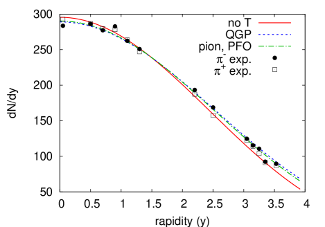
Figure 1: (Color online) Rapidity distribution of charged pions emitted in an Au+Au collision at $\sqrt{s_{NN}}=200$ GeV. The experimental data points are from BRAHMS_PRL . See the text for the explanation of the three theoretical curves.

A comparison of the pion rapidity spectra obtained from the model and the experimental results can be seen on Fig. 1. Three theoretical curves are shown. The first one (labeled “no T”) corresponds to Eq. (25). This is identical to the result of Wong and was obtained by neglecting thermal effects. The second one (“QGP”) shows the result of the calculation taking into account the thermal smearing in the QGP. This curve is the result of the integral (37) where $\tilde{f}$ is the Fermi distribution of massless quarks. Finally, the third one (“pion, PFO”) is calculated from the thermal pion distribution function valid after the phase transition, assuming a pion gas in the post FO side. In the case of the second and third curves the integral (37) was calculated numerically.

Looking at the shape of the obtained rapidity spectra we see that thermal effects improve the precision of coincidence of theoretical and experimental results.

The author of Wong discusses a few possible corrections to the Landau model. One of them is related to the fact that the initial compression of system depends on the EOS, therefore the thickness of the initial state can deviate from the value obtained by taking into account solely the Lorentz contraction of the nuclei. The other possible correction comes from the observation that an arbitrary multiplicative factor can be inserted in the condition of transition to conic flight, Eq. (11), since this equation expresses only a rough equality of the transverse displacement and the transverse system size. Both corrections lead to the modification of the rapidity distribution, Eq. (25), of the form

$$dN/dy\propto\exp\left\{\sqrt{(y_{b}+\zeta)^{2}-y^{2}}\right\},$$ (49)

where the unknown quantity $\zeta$ can be used to improve the agreement of the model and experiment by fitting to the experimental data. Without questioning the validity of these arguments we note here that some of the discrepancies of the Landau model and the experimental data can be explained by the inclusion of thermal effects.

In the case of all three curves on Fig. 1 an overall normalization factor is used following Landau ; Wong as a free parameter and is fitted to the experimental results. This normalization factor, $\mathcal{N}$, is defined by the equation

$$\left.\frac{dN}{dy_{p}}\right|_{\text{normalized}}=\frac{1}{\mathcal{N}}\left.\frac{dN}{dy_{p}}\right|_{\text{primary}},$$ (50)

where $\left(dN/dy_{p}\right)_{\text{primary}}$ is given by Eq. (37). In the case of the first two curves (“no T” and “QGP”) $\mathcal{N}$ has no meaning, since the models do not differentiate between different particle species, and give no prediction for the total pion yield. In the third case (“pion, PFO”) on the other hand the results are obtained from the pion phase-space distribution function, and the value of the normalization can be used to check the validity of the model concerning pion multiplicity.

Using the simple pion gas model for the post FO medium a normalization factor of $\mathcal{N}=9.29$ was obtained, the primary model overestimates the data by this factor. The total four-momentum of the system can be calculated as

$$p_{\text{tot}}^{\mu}=\int T^{\mu\nu}d\sigma_{\nu},$$ (51)

where the integration is over an arbitrary spacelike hypersurface, and the energy-momentum tensor $T^{\mu\nu}$ is given by Eq. (39) with $\epsilon$, $P$ and $u^{\mu}$ as in (4), (3), and (7), respectively. Because of the approximations used in the model the integral Eq. (51) is not independent of the choice of the hypersurface. Specifically, on a surface with constant proper time, $\tau$ the 0th component of (51), the total energy, has the form

$$p_{\text{tot}}^{0}\equiv E_{\text{tot}}=\frac{a^{2}\pi}{4}\tau\int\epsilon\cosh{y}dy,$$ (52)

where in the integration we have used steps similar to those leading to Eq. (21). Calculating the integral Eq. (52) numerically on the FO hypersurface characterized by $\tau=\tau_{FO}=2a$ (see Eq. (11)) for an Au+Au collision at $\sqrt{s_{NN}}=200$ GeV, we get a factor of 5.16 larger value for the total energy in the primary model than the energy of the reaction, A$\sqrt{s_{NN}}$. An overestimation of the pion yield with the same factor is a natural consequence.

In the experimental analysis of BRAHMS_PRL the 5% most central events have been used, while the Landau model pictures an exactly central collision. Based on a simple geometrical model describing the colliding nuclei as spheres with uniformly distributed nucleons the average number of participants in this experimental sample is 88% of the number of participants in a central collision. Assuming that the pion multiplicity scales with the number of participants this means that a model valid for central collisions should give a factor of $1/0.88=1.14$ larger result for the pion multiplicity. Thus, centrality selection and the violation of energy conservation by the Landau hydrodynamical model together explain a normalization factor of $5.16\cdot 1.14=5.88$ in contrast to the value $\mathcal{N}=9.29$ found in the fit to the experimental pion spectra. The remaining discrepancy can be attributed to the fact that the simple pion gas model of the past FO medium can not account for the energy carried by other hadrons. We can conclude that $(5.88/9.29)\cdot 100\%=63\%$ of the energy is carried by pions in the final state of the collision.

In BRAHMS_PRL ratios of the full phase-space extrapolated kaon/pion yields are given. They obtained a value of $0.173\pm 0.017$ for the $K^{+}/\pi^{+}$ ratio and $0.143\pm 0.014$ for the $K^{-}/\pi^{-}$. At midrapidity the density of protons plus antiprotons, $dN_{p+\bar{p}}/dy$ is about half the density of charged kaons, $dN_{K^{+}+K^{-}}/dy$, as can be read off from Fig. 2 of BRAHMS_JPG . From these one can conclude that about 80% of the total charged particles are pions. This value can be consistent with our previous estimate that 63% of total energy is carried by pions, taking into account that – due to their larger mass – kaons and protons carry more energy on average then pions.

We also have to check the validity of the increasing entropy condition, Eq. (42). For that purpose we have to specify the value of the Stefan-Boltzmann constant in the QGP EOS $\epsilon=\sigma T^{4}$. Assuming a mixture of massless quarks/antiquarks and gluons with $N_{f}$ quark flavors and $N_{c}$ colors its value is

$$\sigma=\frac{\pi^{2}}{15}\left(\frac{7N_{f}N_{c}}{4}+N_{c}^{2}-1\right).$$ (53)

Using Eq. (3) we get for the entropy density in the QGP

$$s_{QGP}=\frac{\partial P}{\partial T}=\frac{4}{3}\sigma T^{3}.$$ (54)

We assume a quark-gluon plasma with two quark flavors $N_{f}=2$, and $N_{c}=3$.

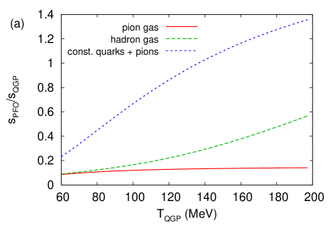
Figure 2: (a) (Color online) The ratio of entropy densities in the hadronic (or post freeze-out; PFO) state and the QGP state as a function of the temperature in QGP. The solid line represents the results obtained assuming a simple pion gas on the hadronic side of the phase transition. The other two curves show the results of the “hadron gas” and “constituent quark/antiquark + pion” gas models. (b) Temperature in the QGP phase at FO in the Landau model as a function of fluid rapidity. Parameters of the initial state correspond to Au+Au collisions at $\sqrt{s_{NN}}=200$ GeV, as described in the text.

Because the four-velocity $u^{\mu}$ is unchanged during the phase transition, the entropy condition (42) is equivalent to $[s]>0$, or $s_{\text{PFO}}/s_{\text{QGP}}>1$, where $s_{\text{QGP}}$ and $s_{\text{PFO}}$ denote the entropy density valid at the quark-gluon plasma and post freeze-out side of the FO hypersurface, respectively. Figure 2 (a) shows the ratio $s_{\text{PFO}}/s_{\text{QGP}}$ as a function of the temperature in QGP. In order to obtain this quantity one has to calculate the post FO temperature in terms of the pre FO (QGP) temperature. This is done using the QGP EOS $\epsilon=\sigma T^{4}$ and inverting numerically the PFO EOS Eq. (44). Then the post FO entropy density is given by Eq. (46).

The continuous curve on Fig. 2 (a) shows that the assumption of the simple pion gas on the hadronic side of the phase transition violates the entropy condition, giving $s_{\text{PFO}}/s_{\text{QGP}}\approx 0.1-0.15$. To understand the reason of this we recall that the entropy carried by free massless particles in an equilibrium ideal gas is a universal constant (3.6 for bosons, 4.2 for fermions), thus, the entropy of the system is proportional to the number of particles. For massive particles the entropy per particle increases but this increase is not very large for pions (see Nonaka ). On the other hand the number of particles decreases significantly. First of all because the degeneracy of states is reduced drastically during the phase transition (from $4N_{F}N_{C}=24$ for quarks plus $N_{C}^{2}-1=8$ for gluons to 3 for pions). Therefore, the available energy has to be distributed among higher energy states allowing for a smaller number of created particles. (Also, some of the available energy is needed to generate the pion mass.)

On Fig. 2 (a) we also plot the entropy density ratio for two other possible models of the hadronic medium already mentioned at the end of Section IV. Including additional hadrons (curve “hadron gas” on the plot) we increase the degeneracy of the states, and also, higher mass hadrons carry more entropy, but the increasing entropy condition is still not fulfilled. On the other hand, the constituent quark/antiquark + pion gas model is consistent with the increasing entropy condition for QGP temperatures $\gtrsim 140MeV$, which is fulfilled for the part of the FO hypersurface where $y\lesssim 3$, as can be seen on Fig. 2 (b). At the edges, where the fluid rapidity is larger, FO happens too late in the Landau model. The increasing entropy condition favors an earlier FO at the sides of the system.

On the other hand, the constituent quark/antiquark + pion gas model describes an intermediate state of the system where hadrons other than pions have not yet been formed. Exactly, the coalescence of quarks to hadrons is the process responsible for the reduction of the number of particles, and, thus, for the usual problems with the increasing entropy condition.

Carrying out the calculation of the pion rapidity distribution assuming the hadron gas model on the post FO side one finds that the shape of the pion rapidity distribution is distorted: there is an enhancement of pion production at large rapidities. The reason for this non-realistic pion rapidity distribution is lying in the assumption of thermal and chemical equilibrium in the post FO medium and the $\tau=\text{const.}$ choice of the FO hypersurface. The FO temperature, that determines the ratio of produced particles of different mass, is not constant along the FO hypersurface (see Fig. 2 (b)). At the side of the fluid with large fluid rapidity the temperature is low, therefore a smaller number of large mass hadrons is created and more energy is left for pion production. This explains the enhanced pion production at large rapidity in this model. A key element in this effect is the presence of large differences between the masses of the particles present in the post FO medium.

We can conclude that the present hadronization description in the Landau model can give a good description of the pion rapidity shape only if the particles in the post FO medium have similar masses.

References

- (1) L. D. Landau, Izv. Akad. Nauk. SSSR 17, 51 (1953).
- (2) S. Z. Belenkij and L. D. Landau, Usp. Fiz. Nauk 56, 309 (1955); Nuovo Cimento Suppl. 3, 15 (1956).
- (3) C. Y. Wong, Phys. Rev. C 78, 054902 (2008).
- (4) F. Cooper and G. Frye, Phys. Rev. D 10, 186 (1974).
- (5) J. Adams et al. (STAR Collaboration), Phys. Rev. Lett. 92, 052302 (2004); S. S. Adler et al. (PHENIX Collaboration), Phys. Rev. Lett. 91, 182301 (2003); A. Adare et al. (PHENIX Collaboration), Phys. Rev. Lett. 98, 162301 (2007).
- (6) D. Molnár and S. A. Voloshin, Phys. Rev. Lett. 91, 092301 (2003); J. Jia and C. Zhang, Phys. Rev. C 75, 031901 (2007).
- (7) I. G. Bearden et al. (BRAHMS collaboration), Phys. Rev. Lett. 94, 162301 (2005).
- (8) M. Murray (BRAHMS collaboration), J. Phys. g 30, S667 (2004).
- (9) C. Nonaka et al., Phys. Rev. C 71 051901(R) (2005).