Anomalous transport resolved in space and time by fluorescence correlation spectroscopy

Abstract

A ubiquitous observation in crowded cell membranes is that molecular transport does not follow Fickian diffusion but exhibits subdiffusion. The microscopic origin of such a behaviour is not understood and highly debated. Here we discuss the spatio-temporal dynamics for two models of subdiffusion: fractional Brownian motion and hindered motion due to immobile obstacles. We show that the different microscopic mechanisms can be distinguished using fluorescence correlation spectroscopy (FCS) by systematic variation of the confocal detection area. We provide a theoretical framework for space-resolved FCS by generalising FCS theory beyond the common assumption of spatially Gaussian transport. We derive a master formula for the FCS autocorrelation function, from which it is evident that the beam waist of an FCS experiment is a similarly important parameter as the wavenumber of scattering experiments. These results lead to scaling properties of the FCS correlation for both models, which are tested by in silico experiments. Further, our scaling prediction is compatible with the FCS half-value times reported by Wawrezinieck et al. [Biophys. J. 89, 4029 (2005)] for in vivo experiments on a transmembrane protein.

Introduction

Measurement of molecular transport at the subcellular level can provide important information on both physiological mechanisms and physical interactions that drive and constrain biochemical processes. The obstructed motion of biomolecules in living cells displays anomalous transport including subdiffusion, which was established in the past decade by numerous experiments applying techniques with labeled particles. Nevertheless, the interpretation of the collected data remains often controversial and the origin of the subdiffusive behaviour is highly debated ^{Szymanski:2009, Magdziarz:2009, He:2008, Lubelski:2008, Saxton:2007, Sung:2006}. Crowded environments like cellular membranes contain structures on many length scales, and further progress depends on experimental techniques that resolve transport on these different scales. Such spatio-temporal information is needed to test and refine models of anomalous transport.

One widespread technique for the investigation of molecular transport is fluorescence correlation spectroscopy (FCS), which follows the motion of fluorescently labeled molecules with high temporal resolution ^{Hess:2002, Schwille:2001}. This mesoscopic, local method consists of collecting the fluorescent light from a steadily illuminated volume or area and autocorrelating its intensity fluctuations. An important parameter of FCS measurements is the beam waist of the illumination laser. While experimental setups in the past were constrained to a fixed value, recent technological advancements allow large variations of the confocal detection area to gather spatial information ^{Gielen:2009, Wawrezinieck:2005, Masuda:2005, Wenger:2007, Hell:2007, Eggeling:2009}. By z-scan FCS ^{Gielen:2009, Wawrezinieck:2005} or beam expanders ^Masuda:2005, focal radii can be varied between 200 nm and 500 nm, but measurements at the nanoscale became possible by introducing nano-apertures (75 nm to 250 nm) ^Wenger:2007. Only lately, a far-field optical nanoscopic method named stimulated emission depletion (STED) fluorescence correlation microscopy was developed to beat the diffraction limit ^Hell:2007, allowing focal radii to span almost a decade down to 15 nm (Ref. Eggeling:2009).

The subdiffusive motion of macromolecules in crowded cells and membranes was studied extensively by FCS experiments ^{Guigas:2007a, Banks:2005, Weiss:2003, Avidin:2010} and was complemented in real-space by single-particle tracking ^{Selhuber-Unkel:2009, Golding:2006, Kusumi:2005, Tolic-Norrelykke:2004}. For Fickian diffusion, the mean-square displacement grows linearly in time, $\delta r^{2}(t)=4Dt$ in two dimensions with diffusion constant $D$. Then, the decay of the FCS autocorrelation function obeys

$$G(t)=\frac{1}{N}\frac{1}{1+t/\tau_{D}}\,,$$ (1)

where $\tau_{D}=w^{2}/4D$ denotes the dwell time and $N$ the average number of labeled molecules in the illuminated area. These equations are no longer valid for anomalous transport. Introducing the walk dimension ${d_{\text{w}}}$, subdiffusion is characterised by $\delta r^{2}(t)\sim t^{2/{d_{\text{w}}}}$, and FCS experiments are often rationalised by

$$G(t)=\frac{1}{N}\frac{1}{1+(\Gamma t)^{\alpha}}$$ (2)

upon fitting $N$, $\Gamma$, and $\alpha$. It is usually and tacitly anticipated that both exponents coincide, $\alpha=2/{d_{\text{w}}}$.

Here, we provide a theoretical framework for space-resolved FCS. Relating the FCS function $G(t)$ to the intermediate scattering function, we generalise the conventionally used fit models and connect FCS to time-resolved scattering techniques. If the beam waist is considered an adjustable experimental parameter similar to the scattering angle, FCS is turned into a valuable tool for the investigation of complex and in particular anomalous transport. The new approach greatly facilitates in silico experiments: for two models of subdiffusion, we show how spatio-temporal information on the tracer dynamics can be obtained and used to distinguish different mechanisms as the origin of anomalous transport.

Theory

Generalised FCS theory.

Let us briefly revisit the theory underlying the FCS technique ^{BernePecora:DynamicLightScattering, Schwille:2001}; we specialise to two dimensions for simplicity. The detection area is illuminated by a laser beam with intensity profile $W(\textrm{r})$. The fluorescent light depends on the fluctuating, local concentration $c(\textrm{r},t)$ of labeled molecules in the laser focus. Thus, the intensity collected at the detector is a spatially weighted average, $I(t)\propto\int\!\mathrm{d}^{2}r\,W(\textrm{r})\,c(\textrm{r},t)$. The output of the FCS experiment is the time-autocorrelation function of the intensity fluctuation $\delta I(t)=I(t)-\left\langle{I}\right\rangle$ around the mean intensity. It is conventionally normalised as $G(t)=\left\langle{\delta I(t)\,\delta I(0)}\right\rangle/\left\langle{I}\right\rangle^{2}$; proper normalisation would be achieved by multiplication with $N=\left\langle{I}\right\rangle^{2}/\left\langle{\delta I^{2}}\right\rangle$. Introducing spatial Fourier transforms, one arrives at the representation

$$G(t;w)=\frac{1}{N}\frac{\int\!\mathrm{d}^{2}q\,|W(\textrm{q})|^{2}\,S(\textrm{q},t)}{\int\mathrm{d}^{2}q\,|W(\textrm{q})|^{2}\,S(\textrm{q},t=0)}\,,$$ (3)

where $S(\textrm{q},t)=\int\!\mathrm{d}^{2}r\,\exp(\text{i}\textrm{q}\boldsymbol{\cdot}\textrm{r})\left\langle{\delta c(\textrm{r},t)\,\delta c(\textrm{0},0)}\right\rangle$ is known as the intermediate scattering function and $W(\textrm{q})$ denotes the Fourier transform of the intensity profile $W(\textrm{r})$.

An conventional laser emits a Gaussian beam profile, $W(\textrm{r})\propto\linebreak[4]\exp\left(-2\textrm{r}^{2}/w^{2}\right)$, with beam waist $w$, which implies a Gaussian filter function $|W(\textrm{q})|^{2}\propto\exp\left(-q^{2}w^{2}/4\right)$. Usually only a small fraction of the molecules is labeled, and then $S(\textrm{q},t)$ reduces to the incoherent intermediate scattering function

$$S(\textrm{q},t)\approx F(\textrm{q},t)=\left\langle{\exp\big{(}\text{i}\textrm{q}\boldsymbol{\cdot}\Delta\textrm{R}(t)\big{)}}\right\rangle\,.$$ (4)

Considering the displacements $\Delta\textrm{R}(t):=\textrm{R}(t)-\textrm{R}(0)$ after a fixed time lag a random variable, the incoherent scattering function can be interpreted as their characteristic function. For Gaussian and isotropic displacements, $\left\langle{\Delta\textrm{R}(t)}\right\rangle=0$, only the second cumulant $\delta r^{2}(t):=\left\langle{|\Delta\textrm{R}(t)|^{2}}\right\rangle$ is non-zero. Thus $F(\textrm{q},t)=\exp\left(-q^{2}\delta r^{2}(t)/4\right)$ for two-dimensional motion. The corresponding FCS function is calculated to

$$G_{\text{Gauss}}(t;w)=\frac{1}{N}\frac{1}{1+\delta r^{2}(t)/w^{2}}\,.$$ (5)

For normal diffusion, it holds $F(\textrm{q},t)=\exp\left(-Dq^{2}t\right)$, and $G(t)$ attains the simple form of Eq. (1). For the case of subdiffusion, $\delta r^{2}(t)\sim t^{\alpha}$, and Gaussian spatial displacements as in fractional Brownian motion (FBM), one recovers the conventional expression, Eq. (2).

In many complex systems, however, the (strong) assumption of Gaussian displacements is not valid and may only serve as an approximation. This assumption can be tested experimentally by resolving the spatial properties of the particle trajectories. An exact expression for the FCS function is obtained by combining equations (3) and (4). Evaluating the integrals over the wavenumber yields

$$G(t;w)=N^{-1}\left\langle{\exp\left(-\Delta\textrm{R}(t)^{2}/w^{2}\right)}\right\rangle\,,$$ (6)

which is a central result of our work. Let us emphasise that it does not require any assumptions on the dynamics; corrections may arise from non-dilute labeling of the molecules and from deviations of the Gaussian beam profile. In three-dimensional systems, one should further correct for anisotropies in the confocal volume. This expression enables new insight in the potential of the FCS technique with consequences for the design of future FCS experiments. The similarity of the representation of $G(t;w)$ in Eq. (6) with that of $F(k,t)$ in Eq. (4) suggests that FCS encodes important spatial information analogous to scattering methods like photon correlation spectroscopy or neutron spin echo. In the case of anomalous transport discussed below, we will use it as starting point for the derivation of the scaling properties of $G(t;w)$. Equation (6) shows that the FCS function $NG(t)$ can be neatly interpreted as the return probability for a fluorescent molecule to be again (or still) in the illuminated area. As a by-product, it provides a simple description for the efficient evaluation of autocorrelated FCS data in computer simulations, circumventing the evaluation of the rapidly fluctuating fluorescent light intensity.

Van Hove correlation function.

The dynamics of a single labeled particle is encoded in the probability distribution of the time-dependent displacements, $P(\textrm{r},t)=\left\langle{\delta(\textrm{r}-\textrm{R}(t)}\right\rangle$; due to rotational symmetry, it actually depends merely on the magnitude $r=|\textrm{r}|$. This function is also known as van Hove (self-)correlation function $G(r,t)$ in the field of liquid dynamics ^{Hansen:SimpleLiquids}; to avoid confusion with the FCS function, we follow the notation of Ref. benAvraham:DiffusionInFractals. Explicit expressions for $P(r,t)$ exist for many models, but for the dynamics on percolation clusters only conjectures of the asymptotic scaling behaviour are available. Let us consider a random walker on the incipient infinite percolation cluster, i.e., precisely at the percolation threshold. Then, the dynamics is characterised by two universal exponents: the fractal dimension ${d_{\text{f}}}$ and the walk dimension ${d_{\text{w}}}$. Let further $t_{0}$ and $\sigma$ denote the typical microscopic time and length scales, respectively. The van Hove function is expected to obey the following scaling law for $r\gg\sigma$ and $t\gg t_{0}$ (Ref. benAvraham:DiffusionInFractals),

$$P_{\infty}(r,t)=r^{-d}\widehat{P}_{\infty}(rt^{-1/{d_{\text{w}}}})\,.$$ (7)

The subscript $\infty$ indicates that the average is taken only for tracers on the infinite cluster. During a time $t$, the walker explores regions of linear extension of the order of $R\sim t^{1/{d_{\text{w}}}}$ . The probability for larger excursions decreases rapidly (presumably like a stretched exponential), hence we assume $\widehat{P}_{\infty}(x\gg 1)\to 0$ rapidly. This property specifies the time evolution of the mean-square displacement and of higher moments. For the FCS measurements, however, we additionally need the limiting behaviour of the scaling function for small arguments.

Return probability.

Integrating the van Hove function over distances $r\leq w$ with $w$ much larger than any microscopic length yields the probability $\Pi(t;w)$ to return to the starting point of the random walk within a radius $w$ after a time $t$. Provided that $w\ll t^{1/{d_{\text{w}}}}$, this probability is proportional to the accessible part of the illuminated area, which scales as $w^{{d_{\text{f}}}}$. In particular, we expect that space- and time-dependence factorise,

$$\Pi(t;w)=\int_{r\leq w}\mathrm{d}^{d}\!r\,P_{\infty}(r,t)\sim w^{{d_{\text{f}}}}\Pi_{0}(t),$$ (8)

where $\Pi_{0}(t)$ denotes the return probability to an infinitesimal vicinity of the origin. By the scaling law Eq. (7), we require that $\widehat{P}_{\infty}(x\ll 1)\sim x^{{d_{\text{f}}}}$, which is confirmed by our simulations for the two-dimensional Lorentz model. As a by-product, one obtains $\Pi_{0}(t)\sim t^{-{d_{\text{f}}}/{d_{\text{w}}}}=t^{-{d_{\text{s}}}/2}$, where ${d_{\text{s}}}=2{d_{\text{f}}}/{d_{\text{w}}}$ is the spectral dimension. Combining both results, $\Pi(t;w)\sim(wt^{-1/{d_{\text{w}}}})^{d_{\text{f}}}$ for sufficiently long times.

Models of anomalous transport

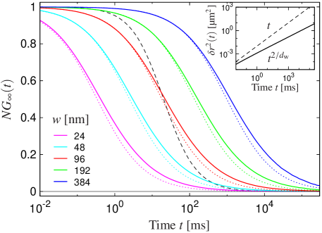
Figure 1: Simulated FCS correlation function $G_{\infty}(t)$ on a logarithmic time axis for tracers on the infinite cluster at the critical obstacle density; the beam waist $w$ of the laser increases from left to right. Dotted lines correspond to FBM with identical mean-square displacement, Eq. (5); the broken line displays the FCS function for unobstructed, normal diffusion ($w=450\,\text{nm}$). Inset: subdiffusive behaviour of the mean-square displacement for the simulated obstructed motion (solid line), again compared to the case of normal diffusion (broken line).

The Lorentz model.

Anomalous transport emerges non-trivially in the Lorentz model ^{Lorentz_PRL:2006, Lorentz_LTT:2007, Lorentz_JCP:2008, Lorentz_2D:2010}. Here, a two-dimensional variant is used which consists of Brownian tracer particles exploring a disordered environment of randomly placed, overlapping circular obstacles of radius $\sigma$, which we choose as $\sigma=3$ nm. The void space between the discs undergoes a continuum percolation transition at the critical obstacle density $n_{c}\sigma^{2}\approx 0.35907$ (Ref. Quintanilla:2000). The infinite cluster displays self-similar behaviour characterised by the fractal dimension ${d_{\text{f}}}=91/48$, known from lattice percolation ^{benAvraham:DiffusionInFractals}. The tracer dynamics on this incipient infinite cluster is found to exhibit subdiffusion, $\delta r^{2}_{\infty}(t)\sim t^{2/{d_{\text{w}}}}$, with walk dimension ${d_{\text{w}}}\approx 2.878$ (Ref. Percolation_EPL:2008), see inset of Fig. 1.

We have generated 1,600 trajectories of Brownian tracers with short-time diffusion coefficient $D_{0}=2.5$ µm²/s, moving on the infinite cluster at criticality. (In practice, we computed trajectories for particles on all clusters and evaluated the time-averaged mean-square displacement for each particle. Then, we selected those particles which did not show localisation based on a criterion for the local exponent of the mean-square discplacement at very long times; only these particles contributed to the final average over independent trajectories.) Taking the divergent length scale into account, we have considered large systems of box length $L=10^{4}\sigma=30$ µm and have run the trajectories up to times of $t\simeq 10^{8}t_{0}$, where $t_{0}=\sigma^{2}/D_{0}=3.6\,$µs is the natural time scale above which the diffusive motion is hindered by obstacles. The resulting correlation functions are invariant under time shift and do not display aging, in agreement with recent FCS experiments on crowded fluids ^{Szymanski:2009}. For the in-silico experiment, we have evaluated the average in Eq. (6) for beam waists between 24 nm and 384 nm.

Fractional Brownian motion.

Fractional Brownian motion (FBM) is a mathematical generalisation of the usual Brownian motion yielding a subdiffusive mean-square displacement, $\delta r^{2}(t)=2dD_{\alpha}t^{\alpha}$, with the generalised diffusion constant $D_{\alpha}$; the distribution of the displacements $\Delta\textrm{R}(t)$ remains Gaussian. The description of a microscopic process generating such a dynamics is challenging, one formulation involving fractional derivatives was given in terms of a generalised Langevin equation ^{Sebastian:1995}. Nevertheless, its “propagator” (van Hove function) can be calculated exactly to

$$P_{\text{FBM}}(r,t)=r^{-d}\,\widehat{P}_{\text{Gauss}}\left(rt^{-\alpha/2}/\sqrt{D_{\alpha}}\right)\,$$ (9)

where $\widehat{P}_{\text{Gauss}}(x)=(2\pi)^{-d/2}x^{d}\exp\bigl{(}-x^{2}/2\bigr{)}$ and $d$ denotes the dimension of space. In particular, it satisfies the scaling form in Eq. (7) exactly. Brownian motion with normal diffusion is obtained in the limit $\alpha\to 1$, where $D_{\alpha}$ becomes the diffusion constant. The FCS function corresponding to FBM is given exactly by Eq. (5). For comparison with the Lorentz model, we have fixed $\alpha$ and $D_{\alpha}$ such that the mean-square displacements of both models coincide.

Results and Discussion

In the following, we will describe how FCS experiments with variable beam waist can provide insight into the microscopic dynamics and reveal spatially non-Gaussian, subdiffusive behaviour. We apply the generalised FCS theory from above to the exactly solvable FBM model and to the two-dimensional Lorentz model with Brownian tracers. We have generated FCS correlation functions as described in the previous section. The obtained curves are shown in Fig. 1 and exhibit a significantly stretched decay compared to normal diffusion. For the corresponding FBM model with identical mean-square displacement, the same trend, but a different shape of $G(t)$ is found. For both models, an increase of the beam waist $w$ shifts the relaxation to later times, while the shape appears to be preserved.

Generalising the diffusion time in Eq. (1), we introduce the half-value time $\tau_{1/2}(w)$ as a function of the beam waist via the implicit definition $NG(\tau_{1/2})=1/2$. The FCS data suggest a phenomenological scaling property, $NG(t;w)=\widetilde{G}\boldsymbol{(}t/\tau_{1/2}(w)\boldsymbol{)}$, i.e., all curves can be collapsed by appropriate rescaling of time. In the following, we will rigorously derive the scaling form of the FCS function $G(t;w)$ for the models under consideration. In particular, a thorough scaling analysis can discriminate whether or not a proposed theoretical model describes the spatio-temporal tracer dynamics contained in the FCS data.