Optimal Co-linear Gaussian Beams for Spontaneous Parametric Down-Conversion

Abstract

I investigate the properties of spontaneous parametric down-conversion (SPDC) involving co-linear Gaussian spatial modes for the pump and the photon collection optics. Approximate analytical and numerical results are obtained for the peak spectral density, photon bandwidth, pair collection probability, heralding ratio, and spectral purity, as a function of crystal length and beam focusing parameters. I address the optimization of these properties individually as well as jointly, and find focusing conditions that simultaneously bring the pair collection probability, heralding ratio, and spectral purity to near-optimal values. These properties are also found to be nearly scale invariant, that is, ultimately independent of crystal length. The results obtained here are expected to be useful for designing SPDC sources with high performance in multiple categories for the next generation of SPDC applications.

I Introduction

Spontaneous parametric down-conversion (SPDC) is a process widely used to produce both entangled photon pairs and heralded single photons. SPDC photon sources play a key role in quantum cryptography, optical quantum computing, quantum metrology, and in fundamental studies of quantum mechanics. In many applications, a nonlinear optical crystal is pumped by a focused laser beam and the emitted SPDC light is collected into a pair of optical waveguides, such as an integrated optical circuit Politi2009_IEEE or a fiber network SECOQC2009 . Efforts over the past decade have led to some very bright SPDC sources Wong2006 ; Fedrizzi2007 . As brightness has improved, interest has progressed from simply making SPDC sources brighter to controlling other properties of the emitted photons, such as the spectral entanglement in each photon pair Grice2001 ; U'Ren2007 ; Mosley2009 ; Humble2007 . While several papers in recent years Kurtsiefer2001 ; Bovino2003 ; Dragan2004 ; Andrews2004 ; Castelletto2005 ; Ljunggren2005 ; Ling2008 ; Kolenderski2009 have addressed the question of how to focus the pump and/or collection optics optimally, some important questions remain. Since different studies have invoked slightly different assumptions and optimized slightly different measures, it is not clear how pump and/or collection focusing simultaneously affects all the quantities that are generally of interest, and what trade-offs (if any) exist between these quantities. Furthermore, the scaling laws for the optimized quantities and optimal parameter values are not readily apparent (e.g. whether it is possible to halve the crystal length and, through a change of beam parameters, obtain similar performance).

To address such questions, I present here a new study of SPDC for the case in which the pump and collecting optics define co-linear Gaussian spatial modes. While the theory is general, the envisioned context is SPDC in a periodically poled nonlinear crystal with emission in the visible or telecommunication spectral range (a common and useful configuration). In this study I consider five properties of the collected biphoton state that are commonly of interest: the joint spectral density; the photon bandwidths; the pair collection probability; the heralding ratio (pair/single photon collection ratio); and the spectral entanglement. These properties are calculated—in some cases analytically, in some cases numerically—as functions of experimental parameters, yielding predictions for the absolute values of the properties as well as for the parameter values that optimize each property. Additionally, this study reveals several scaling laws and shows that some properties can be jointly optimized while others require a trade-off. Many of the results presented here are new, with a few appearing to differ from predictions by others.

The paper is organized as follows: Section II establishes the foundational equations describing Gaussian optical modes and the quantum physics of SPDC. Sections III-VII derive expressions for the five properties mentioned above and discuss their dependence on experimental parameters. Section VIII discusses the results of this study in light of prior works, and Section IX summarizes the main conclusions.

II SPDC with Gaussian Spatial Modes

SPDC is the lowest-order effect of parametric interaction between a strong pump (p) field and two other fields, designated as signal (s) and idler (i), initially in the vacuum state. The quantum Hamiltonian governing this interaction is

$$\hat{H}=\int\varepsilon_{0}\left(\boldsymbol{\chi}^{(2)}(\mathbf{r}):\mathbf{\hat{E}}^{+}(\mathbf{r},t)\mathbf{\hat{E}}^{-}(\mathbf{r},t)\mathbf{\hat{E}}^{-}(\mathbf{r},t)+\text{H.c.}\right)\,d^{3}\mathbf{r}$$ (1)

where $\mathbf{r}=(x,y,z)$ is the spatial coordinate, $t$ is time, $\boldsymbol{\chi}^{(2)}(\mathbf{r})$ is the nonlinear susceptibility tensor, and $\mathbf{\hat{E}}^{+}\mathbf{(r},t)=\mathbf{\hat{E}}^{-}(\mathbf{r},t)^{\dagger}$ is the positive-frequency part of the electric field quantum operator. In canonical treatments, the field is expanded in terms of an orthonormal set of modes. Since the interest here is in SPDC involving Gaussian spatial modes, I choose a modal expansion containing a Gaussian mode for each frequency $\omega$. It will be sufficient to consider just these Gaussian modes until Section VII. In this case $\mathbf{\hat{E}}^{+}(\mathbf{r},t)$ may be written as

$$\mathbf{\hat{E}}^{+}(\mathbf{r},t)=\int_{0}^{\infty}d\omega\sqrt{\frac{\hbar\omega}{4\pi c\varepsilon_{0}}}\mathbf{E}_{\omega}(\mathbf{r})e^{-i\omega t}\hat{a}_{\omega}(t)+\text{irrelevant non-Gaussian modes}$$ (2)

where $\mathbf{E}_{\omega}(\mathbf{r})$ is the electric field function for the (Gaussian) mode of frequency $\omega$ and $\hat{a}_{\omega}^{\dagger}(t)$ is the operator that creates a photon in that mode.

The state resulting from the interaction (1) is obtained by applying the operator $\exp\left[-\frac{i}{\hbar}\int_{-\infty}^{\infty}dt\,\hat{H}(t)\right]$ to the initial state. The part of the state corresponding to SPDC, that is, the creation of a single pair of photons, is just the first-order term:

$$|\Psi_{\text{SPDC}}\rangle=-\frac{i}{\hbar}\int_{-\infty}^{\infty}dt\,\hat{H}(t)\,|\text{initial}\rangle.$$ (3)

Putting (1) and (2) into (3) gives

$$|\Psi_{\text{SPDC}}\rangle=-i\int_{0}^{\infty}d\omega_{\text{s}}d\omega_{\text{i}}\,\psi(\omega_{\text{s}},\omega_{\text{i}})\hat{a}_{\omega_{\text{s}}}^{\dagger}\hat{a}_{\omega_{\text{i}}}^{\dagger}|\text{vac}\rangle$$ (4)

where $|$vac$\rangle$ is the vacuum state of the signal and idler and

$$\psi(\omega_{\text{s}},\omega_{\text{i}})=\sqrt{\frac{2\pi^{2}\hbar N_{\text{p}}}{\varepsilon_{0}\lambda_{\text{p}}\lambda_{\text{s}}\lambda_{\text{i}}}}s(\omega_{\text{p}})\mathcal{O}(\omega_{\text{s}},\omega_{\text{i}})$$ (5)

is the SPDC amplitude. Here $\varepsilon_{0}$ is the vacuum permittivity, $\lambda_{j}=2\pi c/\omega_{j}$ is the free space wavelength of field $j$ ($j=$ p,s,i), and $\omega_{\text{p}}=\omega_{\text{s}}+\omega_{\text{i}}$. The pump field has been assumed to be in a coherent state with independent spectral and spatial dependence. Accordingly, the operator $\hat{a}_{\omega_{\text{p}}}$ has been replaced by the complex amplitude $a(\omega_{\text{p}})=s(\omega_{\text{p}})\sqrt{N_{{}_{\text{p}}}},$ where $s(\omega_{\text{p}})$ is the pump spectral amplitude (with $\int\left|s(\omega)\right|^{2}\,d\omega=1$) and $N_{\text{p}}$ is the mean number of pump photons (the pump energy divided by $\hbar\omega_{\text{p}}$). The quantity

$$\mathcal{O}(\omega_{\text{s}},\omega_{\text{i}})\equiv\int\limits_{\text{medium}}\boldsymbol{\chi}^{(2)}(\mathbf{r}):\mathbf{E}_{\omega_{\text{p}}}(\mathbf{r})\mathbf{E}_{\omega_{\text{s}}}^{\ast}(\mathbf{r})\mathbf{E}_{\omega_{\text{s}}}^{\ast}(\mathbf{r})\mathbf{\,}d^{3}\mathbf{r}$$ (6)

is the spatial overlap of the pump, signal, and idler modes in the medium, which generalizes the $\operatorname{sinc}$ phase matching function encountered in plane-wave treatments of SPDC Hong1985_PRA . The medium is taken to be a bulk material of length $L$ centered at the origin, with cross section large enough to contain the mode functions. The material may be ferroelectrically poled so that $\boldsymbol{\chi}^{(2)}(\mathbf{r})$ alternates sign with spatial period $\Lambda$.

The properties of the SPDC state can be calculated once particular forms are chosen for the pump spectrum $s(\omega_{\text{p}})$ and the mode functions $\mathbf{E}_{\omega_{j}}(\mathbf{r})$. Consideration will be restricted to modes of the form

$$\mathbf{E}(\mathbf{r})=\frac{\mathbf{e}}{\sqrt{\pi/2}}\frac{w}{q}\exp\left[-\frac{x^{2}+y^{2}}{q}+ikz\right]$$ (7)

which describes a linearly polarized, paraxial Gaussian beam with waist at the origin, propagating along the $z$ axis in an optically uniform medium. Here $w$ is the waist size, $\mathbf{e}$ is the polarization unit vector, $k=n\omega/c$ is the wavenumber, $n$ is the refractive index, and $q=w^{2}+2iz/k$. This choice is in part motivated by the fact that some of the best SPDC sources in existence involve Gaussian beams co-propagating along one of the principle refractive axes of a transparent crystalline material, such as potassium titanyl phosphate or lithium niobate. (The anisotropy of the refractive index may be safely ignored in such cases.) Additionally, symmetry indicates that the spatial overlap is largest when the modes co-propagate and have their waists co-located at the center of the crystal. This leaves the waist sizes $w_{\text{p}},w_{\text{s}},w_{\text{i}}$ as the free parameters for mode optimization.

Using modes of the form (7), the mode overlap (6) is

$$\mathcal{O}=\frac{\sqrt{\epsilon}\chi_{\text{eff}}^{(2)}}{\left(\pi/2\right)^{3/2}}\int\frac{w_{\text{p}}w_{\text{s}}w_{\text{i}}}{q_{\text{p}}q_{\text{s}}^{\ast}q_{\text{i}}^{\ast}}\exp\left[-\left(x^{2}+y^{2}\right)\left(\frac{1}{q_{\text{p}}}+\frac{1}{q_{\text{s}}^{\ast}}+\frac{1}{q_{\text{i}}^{\ast}}\right)+i(\Delta k+mK)z\right]\mathbf{\,}dx\,dy\,dz.$$ (8)

Here $\Delta k=k_{\text{p}}-k_{\text{s}}-k_{\text{i}}$ is the wavenumber mismatch, $K=2\pi/\Lambda$ is the poling spatial frequency, $m$ is the order of quasi-phase matching, $\chi_{\text{eff}}^{(2)}\equiv\boldsymbol{\chi}^{(2)}:\mathbf{e}_{\text{p}}\mathbf{e}_{\text{s}}\mathbf{e}_{\text{i}}$ is the effective nonlinear coefficient, and $\epsilon$ is an efficiency factor that includes Fresnel loss and the Fourier coefficient of the $m$th harmonic of the poling spatial function. Integrating over $x$ and $y$ yields

$$\mathcal{O}=\sqrt{\frac{8\epsilon}{\pi}}\chi_{\text{eff}}^{(2)}w_{\text{p}}w_{\text{s}}w_{\text{i}}\int_{-L/2}^{L/2}\frac{\exp\left[i(\Delta k+mK)z\right]}{q_{\text{s}}^{\ast}q_{\text{i}}^{\ast}+q_{\text{p}}q_{\text{i}}^{\ast}+q_{\text{p}}q_{\text{s}}^{\ast}}\,dz.$$ (9)

Before proceeding, it will be convenient to rewrite (9) in terms of dimensionless quantities. The primary independent variables are the phase mismatch

$$\Phi\equiv(\Delta k+mK)L$$ (10)

and the focal parameters

$$\xi_{j}\equiv\frac{L}{k_{j}w_{j}^{2}}$$ (11)

where $\xi_{j}\gg 1$ ($\ll 1$) means that field $j$ ($j=\,$p,s,i ) is focused strongly (weakly) relative to the length of the crystal.

I also define the auxiliary quantities

$$A_{\pm} \equiv 1+\frac{k_{\text{s}}}{k_{\text{p}}}\frac{\xi_{\text{s}}}{\xi_{\text{p}}}\pm\frac{k_{\text{i}}}{k_{\text{p}}}\frac{\xi_{\text{i}}}{\xi_{\text{p}}},$$ (12)

$$B_{\pm} \equiv\left(1-\frac{\Delta k}{k_{\text{p}}}\right)\left(1+\frac{k_{\text{s}}+\Delta k}{k_{\text{p}}-\Delta k}\frac{\xi_{\text{p}}}{\xi_{\text{s}}}\pm\frac{k_{\text{i}}+\Delta k}{k_{\text{p}}-\Delta k}\frac{\xi_{\text{p}}}{\xi_{\text{i}}}\right),$$ (13)

$$C \equiv\frac{\Delta k}{k_{\text{p}}}\frac{\xi_{\text{p}}^{2}}{\xi_{\text{s}}\xi_{\text{i}}}\frac{A_{+}}{B_{+}^{2}},$$ (14)

and the aggregate focal parameter

$$\xi\equiv\frac{B_{+}}{A_{+}}\frac{\xi_{\text{s}}\xi_{\text{i}}}{\xi_{\text{p}}}.$$ (15)

The quantities $A_{+}$, $B_{+},$ and $\xi$ are independent and uniquely determine $\xi_{\text{s}}$, $\xi_{\text{i}}$, and $\xi_{\text{p}}$. $C$ is determined by $A_{+}$ and $B_{+}$. Note that $A_{\pm}$, $B_{\pm}$, and $C$ do not depend on the absolute values of the focal parameters, but on the focus of the signal and idler relative to the pump. In terms of these dimensionless quantities, eq. (5) may be written as

$$\psi(\omega_{\text{s}},\omega_{\text{i}})=\sqrt{\frac{8\pi^{2}\epsilon\hbar n_{\text{s}}n_{\text{i}}N_{\text{p}}L}{\varepsilon_{0}n_{\text{p}}}}\frac{\chi_{\text{eff}}^{(2)}}{\lambda_{\text{s}}\lambda_{\text{i}}}\frac{s(\omega_{\text{p}})}{\sqrt{A_{+}B_{+}}}\int_{-1}^{1}\frac{\sqrt{\xi}\exp\left[i\Phi l/2\right]}{1-i\xi l-C\xi^{2}l^{2}}\,dl.$$ (16)

Eq. (16) will be the starting point for analysis in sections III-VI.

Four approximations will be invoked throughout this work in order to simplify analysis and yield more useful results. These approximations are reasonable for typical bulk SPDC sources, which may be defined to have the following characteristics: the length of the medium is $\gtrsim 1\operatorname{mm}$ and its refractive index is $\gtrsim 1.5$; the parameteric interaction is quasi-phase matched with a first-order grating of period $\Lambda\gtrsim 5\operatorname{\mu m}$; and emission is in the visible or telecommunication spectral range, with $\lambda_{\text{s}}\lesssim 1.6\operatorname{\mu m}$ and $\lambda_{\text{p}}\lesssim 0.8\operatorname{\mu m}$. When assessing the accuracy of approximate formulas, these values will be considered to represent the worst typical case. I will also consider a “reference source” consisting of degenerate type II SPDC in $10\operatorname{mm}$ periodically poled potassiam titanyl phosphyate (PPKTP) with a $750\operatorname{nm}$ pump. This is similar to several sources that have been demonstrated to have good performance Wong2006 ; Fedrizzi2007 ; ORNL_source .

One approximation that will be used liberally is

$$1\pm\frac{\Delta k}{k_{j}}\approx 1.$$ (17)

This approximation is motivated by the fact that efficient SPDC occurs when $\Delta k\approx-mK,$ where $mK/k_{j}$ is typically much smaller than 1.

Another approximation that will prove convenient is

$$C\approx 0.$$ (18)

The actual value of $C$ depends in a complicated way upon the experimental parameters, but can be shown to obey the bound

$$\left|C\right|\leq\frac{\left|\Delta k\right|k_{\text{p}}}{4k_{\text{s}}k_{\text{i}}}=\left|\frac{\Phi k_{\text{p}}}{4k_{\text{s}}k_{\text{i}}L}-\frac{mKk_{\text{p}}}{4k_{\text{s}}k_{\text{i}}}\right|$$ (19)

when (17) is valid. One then has $|C|\lesssim 0.1$ near phase matching conditions, which turns out to be small enough to make (18) a fair approximation over the range of focusing that is desirable with respect to the five properties of the state considered here.

The third approximation is that the frequency dependence of (16) is determined essentially by the pump spectrum $s(\omega_{\text{p}})$ and the frequency dependence of the wave mismatch $\Delta k$. That is, I take

$$A_{\pm},B_{\pm},\xi_{j},\sqrt{\frac{\epsilon n_{\text{s}}n_{\text{i}}}{n_{\text{p}}}}\frac{\chi_{\text{eff}}^{(2)}}{\lambda_{\text{s}}\lambda_{\text{i}}}\approx\text{constant}$$ (20)

over the range of $(\omega_{\text{s}},\omega_{\text{i}})$ for which the amplitude is appreciable. For (20) to hold, the bandwidths of the photons must be much smaller than an optical frequency. Type II and non-degenerate type I SPDC sources typically satisfy this condition, but frequency-degenerate type I sources and sources made of very short crystals, which tend to have large bandwidths, may not.

Finally, after section III it will be assumed the wave mismatch $\Delta k$ has a predominantly linear frequency dependence:

$$\delta k_{j}\approx\frac{n_{j}^{\prime}}{c}\delta\omega_{j}$$ (21)

where $n_{j}^{\prime}\equiv c\,\partial k_{j}/\partial\omega$ is the group index of mode $j$ and $\delta\omega_{j}$ $(\delta k_{j})$ denotes a shift from the nominal frequency (wavenumber) of mode $j$. Again, this approximation is generally valid for type II and non-degenerate type I SPDC sources, but not for frequency-degenerate type I sources.

The impact of these approximations, particularly (18), will be addressed more fully in the context of each major result.

III Joint Spectral Density

The joint spectral density $\left|\psi(\omega_{\text{s}},\omega_{\text{i}})\right|^{2}$ is the expected number of photons pairs, per signal bandwidth per idler bandwidth, emitted into the Gaussian collection modes. If the collected photons pass through spectral filters of narrow bandwidth, the effective brightness of the source is determined by the joint spectral density at the filter frequencies. Let us now consider the problem of maximizing this quantity, that is, finding the values of $\xi_{\text{p}},\xi_{\text{s}},\xi_{\text{i}},\Phi$ that maximize $\left|\psi(\omega_{\text{s}},\omega_{\text{i}})\right|^{2}$ given the frequencies $\omega_{\text{p}},\omega_{\text{s}},\omega_{\text{i}}$ and crystal length $L$. From (16), it is apparent that maximization determines certain values $(A_{+}^{\text{max}},B_{+}^{\text{max}},\xi^{\text{max}},\Phi^{\text{max}})$. The beam parameters $\xi_{\text{p}},\xi_{\text{s}},\xi_{\text{i}}$ are then complicated functions of $(k_{\text{p}},k_{\text{s}},k_{\text{i}},A_{+}^{\text{max}},B_{+}^{\text{max}},\xi^{\text{max}},\Phi^{\text{max}})$ via relations (10)-(15). However, substantially more informative results can be obtained if the $l^{2}$ term in (16) is neglected. With $C\approx 0$ (approximation (18)), the function to be maximized is

$$\frac{1}{\sqrt{A_{+}B_{+}}}\times\int_{-1}^{1}\frac{\sqrt{\xi}\exp\left[i\Phi l/2\right]}{1-i\xi l}\,dl.$$ (22)

The two factors are independent and can be maximized separately. $A_{+}B_{+}$ can be written as

$$A_{+}B_{+}=\left(1-\frac{\Delta k}{k_{\text{p}}}\right)\left(1+X_{\text{s}}r_{\text{s}}+X_{\text{i}}r_{\text{i}}\right)\left(1+\frac{X_{\text{s}}}{r_{\text{s}}}+\frac{X_{\text{i}}}{r_{\text{i}}}\right)$$

where

$$X_{j} \equiv\frac{k_{j}}{k_{\text{p}}}\sqrt{\frac{1+\Delta k/k_{j}}{1-\Delta k/k_{\text{p}}},}$$ (23)

$$r_{j} \equiv\frac{\xi_{j}}{\xi_{\text{p}}}\sqrt{\frac{1-\Delta k/k_{\text{p}}}{1+\Delta k/k_{j}}}.$$ (24)

The maximum of $\left(A_{+}B_{+}\right)^{-1/2}$ occurs at $r_{\text{s}}=r_{\text{i}}=1$. Invoking approximation (17) gives

$$\xi_{\text{s}}\approx\xi_{\text{i}}\approx\xi_{\text{p}}\approx\xi$$ (25)

and

$$\max\frac{1}{\sqrt{A_{+}B_{+}}}\approx\frac{1}{2}.$$ (26)

The second factor in (22),

$$F(\xi,\Phi)\equiv\int_{-1}^{1}\frac{\sqrt{\xi}\exp\left[i\Phi l/2\right]}{1-i\xi l}\,dl$$ (27)

requires numerical evaluation and is plotted in Fig. 1. (Note that for $\xi\ll 1,$ $F$ is proportional to the usual phase matching function $\operatorname{sinc}(\Phi/2)$.) The maximum value of $F$ is $2.06\cdots$ at $\xi=2.84\cdots$, $\Phi=-(1.04\cdots)\pi$. This result, together with (26), yields the maximum spectral amplitude

$$\max_{\xi,\Phi}\left|\psi(\omega_{\text{s}},\omega_{\text{i}})\right|\approx 1.03\sqrt{\frac{8\pi^{2}\hbar\epsilon n_{\text{s}}n_{\text{i}}}{\varepsilon_{0}n_{\text{p}}}}\frac{\chi_{\text{eff}}^{(2)}}{\lambda_{\text{s}}\lambda_{\text{i}}}\sqrt{N_{\text{p}}L}s(\omega_{\text{p}})$$ (28)

which is obtained under the conditions

$$\left.\xi_{\text{s}}\approx\xi_{\text{i}}\approx\xi_{\text{p}}\right. \approx 2.84,$$ (29)

$$\Phi \approx-1.04\pi.$$ (30)

It should be noted that these are precisely the conditions which have long been known to maximize the efficiency of sum frequency generation and parametric amplification with Gaussian beams Boyd1968 . The spectral density $\left|\psi(\omega_{\text{s}},\omega_{\text{i}})\right|^{2}$ is proportional to the number of pump photons $N_{\text{p}}$ and to the crystal length. (In contrast, for the case of collimated (plane wave) interaction, the spectral density would grow quadratically with the crystal length.) It may also be noted that, for all other factors being equal, short-wavelength sources are brighter than long-wavelength sources.

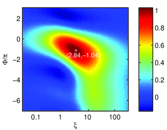
Figure 1: (color online) The spatial overlap factor $F(\xi,\Phi)$ defined in eq. (27). The cross marks the location of the peak.

Since it may not always be possible to implement or verify condition (29) accurately, it is worth examining how sensitive the peak spectral density is to the focal parameters. Specifically, I compare $\max_{\Phi}\left|\psi\right|^{2},$ which is a function of $(\xi_{\text{p}},\xi_{\text{s}},\xi_{\text{i}}),$ to the global maximum value $\max_{\xi,\Phi}\left|\psi\right|^{2}$. I constrain the parameter space by the condition $\xi_{\text{s}}=\xi_{\text{i}},$ which is not only optimal in regard to the spectral density, but as will be shown in later sections, is also optimal or near-optimal for other quantities of interest. Fig. 2 shows the relative brightness $\max_{\Phi}\left|\psi\right|^{2}/\max_{\xi,\Phi}\left|\psi\right|^{2}$ as a function of $\xi_{\text{p}}$ and $\xi_{\text{s}}=\xi_{\text{i}}$. It can be seen that the regime of good focusing is rather broad: the waist size (and correspondingly, the angular divergence) must be made smaller or larger by roughly a factor of 5 to reduce the peak spectral density to half its maximum value. Over this range the optimal phase $\Phi$ (not shown) varies from $-\pi/2$ to $-3\pi/2,$ meaning that the frequency of the peak shifts slightly with focusing. If the signal and idler focus are fixed, the optimal pump focus is given by $\xi_{\text{p}}=\xi_{\text{s}}(=\xi_{\text{i}})$. However, if the pump focus is fixed, the optimal signal and idler focus are given by $\xi_{\text{s}}=\xi_{\text{i}}\approx\sqrt{2.84\xi_{\text{p}}}$.

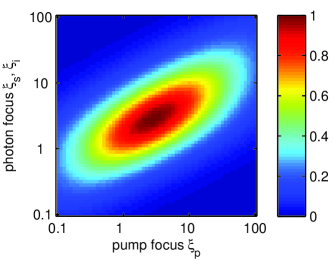
Figure 2: (color online) Peak joint spectral density, normalized to the global maximum, as a function of the pump and photon mode focus.

These results are robust to approximation: for the worst case defined in section II, the “optimal” values given in (29) and (30) differ from the true optimal values by 5% and 10% respectively, but, due to the broadness of $\psi$ as a function of these parameters, yield an amplitude that is within 1% of the actual maximum value.

IV Photon Bandwidth with Monochromatic Pumping

SPDC photons are sometimes employed in systems with limited optical bandwidth. In designing sources for such systems it is helpful to know how the photon bandwidths depend on the design parameters. One case of particular interest is when the pump bandwidth is chosen to maximize the spectral purity of the photons. That case will be addressed in section VI. Another particularly interesting case is that of monochromatic pumping, which will be addressed now.

With a monochromatic pump, and under approximation (20), the spectral dependence of (16) arises primarily from the dispersion of the phase mismatch $\Phi=(\Delta k+mK)L$. The phase mismatch may be expanded as Taylor series in $\delta\omega_{\text{s}}$ and $\delta\omega_{\text{i}}$, the deviation of the signal and idler frequencies from their nominal values. Assumption (21) then gives

$$\Phi\approx\Phi_{0}+\left(\frac{n_{\text{p}}^{\prime}}{c}(\delta\omega_{\text{s}}+\delta\omega_{\text{i}})-\frac{n_{\text{s}}^{\prime}}{c}\delta\omega_{\text{s}}-\frac{n_{\text{i}}^{\prime}}{c}\delta\omega_{\text{i}}\right)L$$ (31)

where $\Phi_{0}$ is the phase mismatch at the nominal frequencies. Monochromatic pumping constrains the frequencies to $\delta\omega_{\text{s}}=-\delta\omega_{\text{i}},$ yielding

$$\Phi\approx\Phi_{0}+\frac{(n_{\text{s}}^{\prime}-n_{\text{i}}^{\prime})L}{c}\delta\omega_{\text{s}}.$$ (32)

The fact that $\Phi$ is (approximately) a linear function of $\omega_{\text{s}}$ means that the photon bandwidth $\Delta\omega_{\text{s}}$ ($=\Delta\omega_{\text{i}}$) can be expressed in terms of a dimensionless “phase mismatch bandwidth” $\Delta\Phi$, which is the width of $|\psi|^{2}$ when expressed as function of $\Phi$.

Under approximation $C\approx 0$, $|\psi|^{2}$ is proportional to $|F(\xi,\Phi)|^{2}$. The full-width at half maximum (FWHM) of $\left|F(\xi,\Phi)\right|^{2}$ (see Fig. 1) was calculated numerically and is plotted as the solid line in Fig. 3. I find that the behavior of $\Delta\Phi$ in this case is captured well by the heuristic formula

$$\Delta\Phi\sim 2\pi\max(1,\xi/10),$$ (33)

shown as the dashed line. Combining (32) and (33) yields the photon bandwidths

$$\Delta\omega_{\text{s}}=\Delta\omega_{\text{i}}\sim\frac{2\pi c}{\left|n_{\text{s}}^{\prime}-n_{\text{i}}^{\prime}\right|}\max\left(\frac{1}{L},\frac{1}{10b}\right)$$ (34)

where $b\equiv L/\xi$ is the aggregate confocal length of the modes (reducing to $k_{\text{p}}w_{\text{p}}^{2}$ when $\xi_{\text{s}}=\xi_{\text{i}}=\xi_{\text{p}}$). When focusing is weak to moderate ($\xi\lesssim 10$), the photon bandwidth is determined by the crystal length (the well-known $1/L$ dependence). But when the focusing is strong ($\xi\gtrsim 10$), the bandwidth is larger Carrasco2006 and determined instead by the confocal length, going as $1/b$.

The reason that tightly focusing the pump increases the bandwidth can be understood as follows: At negative values of the phase mismatch (i.e. away from the nominal wavelengths), the photon spatial distribution in the far field takes the form of a ring Kwiat1995 . With a collimated pump, a certain change in wavelength makes the ring radius larger than that of the collection modes, and photons of those wavelengths are not collected. But when the pump is tightly focused, the rings are spatially broadened and the photons partially overlap the collection mode Zhao2008 . The larger the spatial broadening, the larger the wavelength change must be for the photon distribution to lie outside the collection mode.

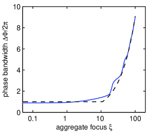
Figure 3: (color online) The normalized photon bandwidth as a function of focusing. The dashed line is the heuristic formula (33).

Due to the approximation $C=0$, the bandwidth plotted in Fig. 3 is not exact. For the reference source, the error in $\Delta\omega_{\text{s}}$ is $\leq 3\%$ for $\xi\leq 10$ and $\leq 10\%$ over the range $10\leq\xi_{\text{p}}\leq 100$. For the worst typical case, the error is $\leq 3\%$ for $\xi\leq 1,$ but increases to $10\%$ at $\xi=10$ and varies between $30\%$ and $50\%$ over the range $10\leq\xi_{\text{p}}\leq 100$. Thus bandwidth predictions may not be highly accurate in the regime of focus-induced spectral broadening. Nevertheless, even in the worst case the approximate SPDC state $|\tilde{\psi}\rangle$ (calculated with $C=0$) has a large overlap with the exact state $|\psi\rangle$ (calculated using (19)): the fidelity $\langle\tilde{\psi}|\psi\rangle^{2}/\langle\tilde{\psi}|\tilde{\psi}\rangle\langle\psi|\psi\rangle$ is 0.999 at $\xi=1,$ 0.97 at $\xi=10,$ and 0.91 at $\xi=100$. Also, the heuristic formula $\Delta\Phi\sim 2\pi\max(1,\xi/\xi_{0})$ remains as accurate as shown in Fig. 3 for a suitably chosen value of $\xi_{0}$.

V Pair Collection Probability

When SPDC photons are collected without spectral filtering, maximizing the pair collection probability

$$P_{\text{si}}=\int\left|\psi(\omega_{\text{s}},\omega_{\text{i}})\right|^{2}d\omega_{\text{s}}d\omega_{\text{i}}.$$ (35)

is usually more important than maximizing the peak spectral density. (In most experiments, $P_{\text{si}}$ is proportional to the coincident photodection rate, or the probability of detecting a pair of photons following any given pump pulse.) Under approximation (20), the dominant spectral dependence arises from $s(\omega_{\text{p}})$ and $\Delta k$. The phase mismatch (31) may be written as

$$\Phi\approx\Phi_{0}+\left(\frac{2n_{\text{p}}^{\prime}-(n_{\text{s}}^{\prime}+n_{\text{i}}^{\prime})}{2c}\delta\omega_{\text{p}}-\frac{n_{\text{s}}^{\prime}-n_{\text{i}}^{\prime}}{2c}\delta\omega_{-}\right)L$$ (36)

where $\omega_{-}=\omega_{\text{s}}-\omega_{\text{i}}$. Then $d\omega_{\text{s}}d\omega_{\text{i}}=(d\omega_{-}d\omega_{\text{p}})/2=d\Phi d\omega_{\text{p}}\,c/(|n_{\text{s}}^{\prime}-n_{\text{i}}^{\prime}|L)$, giving

$$P_{\text{si}} =\frac{c}{\left|n_{\text{s}}^{\prime}-n_{\text{i}}^{\prime}\right|L}\int\left|\psi\right|^{2}\,d\omega_{\text{p}}d\Phi$$ (37)

$$=\frac{8\pi^{2}\hbar c\epsilon n_{\text{s}}n_{\text{i}}}{\varepsilon_{0}n_{\text{p}}\left|n_{\text{s}}^{\prime}-n_{\text{i}}^{\prime}\right|}\left(\frac{\chi_{\text{eff}}^{(2)}}{\lambda_{\text{s}}\lambda_{\text{i}}}\right)^{2}\frac{N_{\text{p}}}{A_{+}B_{+}}\int\left|s(\omega_{\text{p}})\int_{-1}^{1}\frac{\sqrt{\xi}\exp\left[i\Phi l/2\right]}{1-i\xi l-C\xi^{2}l^{2}}\,dl\right|^{2}d\omega_{\text{p}}d\Phi.$$ (38)

Under the approximation $C\approx 0$, the only place $\Phi$ appears is in the exponential function. Using $\int\exp\left[i\Phi(l-l^{\prime})/2\right]\,d\Phi=4\pi\delta(l-l^{\prime})$ and $\int\left|s(\omega_{\text{p}})\right|^{2}d\omega_{\text{p}}=1,$ one obtains

$$P_{\text{si}}\approx\frac{32\pi^{3}\hbar c\epsilon n_{\text{s}}n_{\text{i}}}{\varepsilon_{0}n_{\text{p}}\left|n_{\text{s}}^{\prime}-n_{\text{i}}^{\prime}\right|}\left(\frac{\chi_{\text{eff}}^{(2)}}{\lambda_{\text{s}}\lambda_{\text{i}}}\right)^{2}\frac{N_{\text{p}}\xi}{A_{+}B_{+}}\int_{-1}^{1}\frac{dl}{1+\xi^{2}l^{2}}$$ (39)

which may be directly integrated to give

$$P_{\text{si}}\approx\frac{64\pi^{3}\hbar c\epsilon n_{\text{s}}n_{\text{i}}}{\varepsilon_{0}n_{\text{p}}\left|n_{\text{s}}^{\prime}-n_{\text{i}}^{\prime}\right|}\left(\frac{\chi_{\text{eff}}^{(2)}}{\lambda_{\text{s}}\lambda_{\text{i}}}\right)^{2}\frac{\arctan\left(\xi\right)}{A_{+}B_{+}}N_{\text{p}}.$$ (40)

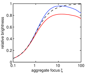
Figure 4: (color online) Dependence of the pair collection probability on the aggregate focus. The dashed line is eq. (40) normalized by its asymptotic maximum. The solid lines are calculated using “worst case” values for the parameter $C$ (see discussion surrounding eq. (19)) and normalized by the same factor.

Formula (40), plotted as the dashed line in Fig. 4, suggests that the pair probability can only be optimized in an asymptotic sense—that there are no finite values of $\xi_{\text{p}},\xi_{\text{s}},\xi_{\text{i}}$ that maximize $P_{\text{si}}$. In reality, the asymptotic behavior holds only as long as $\xi k_{\text{p}}/(4Lk_{\text{s}}k_{\text{i}})\lesssim 0.1$. With very tight focusing or very short crystals, the approximation $C=0$ breaks down, causing $P_{\text{si}}$ to peak near its asymptotic value (solid lines in Fig. 4). In the worst typical case the pair probability error $\left|1-\langle\tilde{\psi}|\tilde{\psi}\rangle/\langle\psi|\psi\rangle\right|$ is $\leq 4\%$ for $\xi\leq 1,$ $\leq 13\%$ for $\xi\leq 10,$ and $\leq 20\%$ for $\xi\leq 100$. For the reference source described above, the pair probability error is $\leq 1.5\%$ for $\xi\leq 100$. In any case, $P_{\text{si}}$ evidently has an upper bound

$$P_{\text{si}}\leq\frac{8\pi^{4}\hbar c\epsilon n_{\text{s}}n_{\text{i}}}{\varepsilon_{0}n_{\text{p}}\left|n_{\text{s}}^{\prime}-n_{\text{i}}^{\prime}\right|}\left(\frac{\chi_{\text{eff}}^{(2)}}{\lambda_{\text{s}}\lambda_{\text{i}}}\right)^{2}N_{\text{p}}$$ (41)

that cannot be exceeded, no matter how long the crystal. (This somewhat surprising result will be discussed in section VIII.) For type II SPDC sources made of PPKTP or periodically poled lithium niobate (PPLN), eq. (41) predicts that brightnesses exceeding $10^{-9}$ collected pairs/pump photon should be achievable—roughly an order of magnitude brighter than the brightest existing sources.

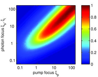
Figure 5: (color online) Dependence of the pair collection probability on the focus of the pump and photon modes.

The dependence of $P_{\text{si}}$ on $\xi_{\text{p}}$ and $\xi_{\text{s}}=\xi_{\text{i}}$ is shown in Fig. 5. If the signal and idler focus are fixed, the optimal pump focus is given by $\xi_{\text{p}}=\xi_{\text{s}}(=\xi_{\text{i}})$. If instead $\xi_{\text{p}}$ is fixed, the optimal value of $\xi_{\text{s}}$ is nearly equal to $\xi_{\text{p}}$ for $\xi_{\text{p}}\gtrsim 10$ and slightly larger than $\xi_{\text{p}}$ for $\xi_{\text{p}}\lesssim 10$.

VI Spectral Purity

A number of applications of SPDC photons, including the generation of multiphoton entangled states for quantum computing Lu2007 ; Radmark2009 ; Wieczorek2009 ; Prevedel2009 , involve interference between photons from separate (and nominally identical) SPDC sources. The success of such applications depends not only on the efficiency of SPDC photon production, but also on the degree of mutual coherence of photons from independent sources U'Ren2003 ; Humble2008 . This coherence, which is directly related to the interference visibility, is given by the single-photon purity

$$\rho=\frac{\sum_{j}\sigma_{j}^{2}}{\left(\sum_{j}\sigma_{j}\right)^{2}}$$ (42)

where

$$\psi(\omega_{\text{s}},\omega_{\text{i}})=\sum_{j}\sqrt{\sigma_{j}}u_{j}(\omega_{\text{s}})v_{j}(\omega_{\text{i}})$$ (43)

is the Schmidt decomposition Law2000 of the collected biphoton state. The single-photon purity is inversely related to the degree of entanglement between the signal and idler frequencies, with $\rho=1$ corresponding to no spectral entanglement. (Note that any spatial entanglement present in the emitted state is discarded upon post-selecting photon pairs that couple into the Gaussian collection modes.)

It is natural to ask whether the parameters that yield high source brightness also yield high spectral purity. Under approximations (20) and (21), the frequency-dependent part of $\psi(\omega_{\text{s}},\omega_{\text{i}})$ is $s(\omega_{\text{p}})F(\xi,\Phi)$. Since the purity depends only on the shape of $\psi(\omega_{\text{s}},\omega_{\text{i}}),$ and not on its location or extent within the $(\omega_{\text{s}},\omega_{\text{i}})$ plane, $\omega_{\text{s}}$ and $\omega_{\text{i}}$ may be replaced with the dimensionless variables $\omega_{\text{s}}/\Omega$ and $\omega_{\text{i}}/\Omega$, where $\Omega\equiv c/(n_{\text{s}}^{\prime}-n_{\text{i}}^{\prime})L$. Given a particular functional form for the pump spectrum, the purity may then be computed as a function of $(\xi,\theta,\Delta\omega_{\text{p}}/\Omega)$ where $\Delta\omega$ is the pump bandwidth and

$$\tan\theta=\frac{n_{\text{s}}^{\prime}-n_{\text{p}}^{\prime}}{n_{\text{p}}^{\prime}-n_{\text{i}}^{\prime}}$$ (44)

is the slope, in the $(\omega_{\text{s}},\omega_{\text{i}})$ plane, of the line characterized by $\Phi=0$. Note that since $\xi$ is the only relevant focusing parameter, we are free to set $\xi_{\text{s}}\approx\xi_{\text{i}}\approx\xi_{\text{p}}$ to maximize the brightness at a given $(\xi,\theta,\Delta\omega_{\text{p}}/\Omega)$. Also, note that the brightness is independent of pump bandwidth when approximation (21) is valid.

The spectral purity obtainable with a Gaussian pump was determined by computing $s(\omega_{\text{p}})F(\xi,\Phi)$ over a grid of sufficient extent and resolution in the $(\omega_{\text{s}}/\Omega,\omega_{\text{i}}/\Omega)$ plane for various parameter values $(\xi,\theta,\Delta\omega_{\text{p}}/\Omega)$. For each set of parameter values, singular value decomposition was applied to the matrix of computed values to determine $\{\sigma_{j}\}$ and $\rho$. Numerical optimization was then used to determine the value of $\Delta\omega_{\text{p}}/\Omega$ that maximizes $\rho$ at each $(\xi,\theta)$. In Fig. 6 these optimized values of $\rho$ are plotted as a function of $\xi$ $(=\xi_{\text{p}})$ for several different values of $\theta$. For $\theta=45^{\circ}$, the peak purity is 0.94 and occurs at $\xi=2.2$. As $\theta$ decreases to $0^{\circ}$, $\rho$ asymptotically increases to 1 for all values of $\xi$, although the optimal pump bandwidth becomes infinite in this limit. Below $0^{\circ}$, $\rho$ drops rapidly. Solutions for $\theta\geq 45^{\circ}$ mirror those for $\theta\leq 45^{\circ}$, with the signal and idler exchanging roles.

These results can be understood as follows. The purity is directly related to the factorability of $\psi(\omega_{\text{s}},\omega_{\text{i}})\propto s(\omega_{\text{p}})F(\xi,\Phi)$ into separate functions of $\omega_{\text{s}}$ and $\omega_{\text{i}}$. When the pump function $s(\omega_{\text{p}})$ is Gaussian, complete factorability can be achieved if and only if the phase matching function $F(\xi,\Phi)$ is also Gaussian with orientation $0\leq\theta\leq\pi/2$ Grice2001 . But $F(\xi,\Phi)$ is not Gaussian: for $\xi\ll 1$ it is a $\operatorname{sinc}$ function, which has oscillating side lobes, while for $\xi\gg 1$ it has large skew. In both these regimes, the purity is reduced. $F(\xi,\Phi)$ is most nearly Gaussian for $\xi\sim 2$, which becomes the regime of greatest purity.

Comparing with Figs. 2 and 4, one sees that in the regime of peak purity ($\xi\sim 2$), the spectral intensity is close to its peak value and the total collection probability is more than 70% of its asymptotic maximum (41). Thus, high spectral purity ($\geq 94\%$) can be obtained with focusing conditions that also yield relatively high brightness, provided $0\leq\theta\leq 90^{\circ}$ (which amounts to the requirement that $n_{\text{p}}^{\prime}$ lie between $n_{\text{s}}^{\prime}$ and $n_{\text{i}}^{\prime}$).

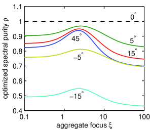
Figure 6: (color online) Dependence of the spectral purity of the collected photons on the mode focus. The numbers accompanying each line are the group velocity angle $\theta$ defined in eq. (44). Solutions for $\theta\geq 45^{\circ}$ mirror those for $\theta\leq 45^{\circ}$.

An explicit evaluation of the accuracy of these results in view of approximation (18) was not performed. However, it may be noted that the results of this section are based on a decomposition of an approximate state which, as discussed at the end of section IV, has a high degree of overlap with the actual state.

VII Single-Photon Collection and Heralding Ratio

In some applications of SPDC, the detection of a photon in the signal mode is used to indicate the (probable) presence of a photon in the idler mode. (Although the photons are always emitted in pairs, conditions generally allow one photon to be emitted into a spatial mode defined by the collection optics while its partner is emitted into a non-collected spatial mode.) In such applications it is desirable to have a high heralding ratio $\eta_{\text{s}}\equiv P_{\text{si}}/P_{\text{s}},$ where $P_{\text{s}}$ is the probability that a photon is emitted into the signal collection mode, regardless of the mode its partner is in. Since the probability of collecting both photons cannot exceed the probability of collecting one of the photons, the heralding ratio can be at most unity. In applications that treat signal and idler photons symmetrically, the quantity $\eta_{\text{si}}\equiv P_{\text{si}}/\sqrt{P_{\text{s}}P_{\text{i}}}$ is often the metric of choice. In this work $\eta_{\text{s}}$ will be called the signal heralding ratio and $\eta_{\text{si}}$ will be called the symmetric heralding ratio.

To obtain the signal collection probability $P_{\text{s}},$ the joint collection probability must be summed over a complete set of spatial modes for the idler photon. The Laguerre-Gauss modes

$$\mathbf{E}^{(n,l)}(\mathbf{r};\omega)=\frac{\mathbf{e}}{\sqrt{\pi/2}}\left(\frac{w_{\text{i}}}{q_{\text{i}}}\right)^{l+1}\left(\frac{q_{\text{i}}^{\ast}}{q_{\text{i}}}\right)^{n}L_{n}^{l}\left(\frac{2w_{\text{i}}^{2}\rho^{2}}{\left|q_{\text{i}}\right|^{2}}\right)\exp\left[-\frac{\rho^{2}}{q_{\text{i}}}+ik_{\text{i}}z+il\phi\right]$$ (45)

form such a set, where $L_{n}^{l}$ is the $(n,l)$ associated Laguerre polynomial, $\rho=\sqrt{x^{2}+y^{2}},$ and $\tan\phi=x/y$. The fundamental mode with $n=l=0$ is just the Gaussian mode introduced in section II. Since the pump and signal mode are azimuthally symmetric, the spatial overlap vanishes unless the idler mode is also azimuthally symmetric ($l=0$). Thus the spatial overlap involving the $n$th idler mode is

$$\mathcal{O}_{n}=\frac{\sqrt{\epsilon}\chi_{\text{eff}}^{(2)}}{\left(\pi/2\right)^{3/2}}\int_{-L/2}^{L/2}\int_{0}^{\infty}\frac{w_{\text{p}}w_{\text{s}}w_{\text{i}}}{q_{\text{p}}q_{\text{s}}^{\ast}q_{\text{i}}^{\ast}}\left(\frac{q_{\text{i}}}{q_{\text{i}}^{\ast}}\right)^{n}L_{n}\left(\frac{2w_{\text{i}}^{2}\rho^{2}}{\left|q_{\text{i}}\right|^{2}}\right)\\ \times\exp\left[-\rho^{2}\left(\frac{1}{q_{\text{p}}}+\frac{1}{q_{\text{s}}^{\ast}}+\frac{1}{q_{\text{i}}^{\ast}}\right)+i(\Delta k+mK)z\right]2\pi\rho\,d\rho\,dz.$$ (46)

With the Laguerre polynomial expansion formula $L_{n}(x)=\sum_{j=0}^{n}(-1)^{j}\frac{n!}{(n-j)!j!j!}x^{j}$ and a bit of work, one can obtain

$$\mathcal{O}_{n}=\sqrt{\frac{8\epsilon}{\pi}}\chi_{\text{eff}}^{(2)}w_{\text{p}}w_{\text{s}}w_{\text{i}}\int_{-L/2}^{L/2}\frac{\exp\left[i(\Delta k+mK)z\right]}{q_{\text{s}}^{\ast}q_{\text{i}}^{\ast}+q_{\text{p}}q_{\text{i}}^{\ast}+q_{\text{p}}q_{\text{s}}^{\ast}}\left(\frac{q_{\text{s}}^{\ast}q_{\text{i}}+q_{\text{p}}q_{\text{i}}-q_{\text{p}}q_{\text{s}}^{\ast}}{q_{\text{s}}^{\ast}q_{\text{i}}^{\ast}+q_{\text{p}}q_{\text{i}}^{\ast}+q_{\text{p}}q_{\text{s}}^{\ast}}\right)^{n}dz.$$ (47)

Applying definitions (10)-(14) and making the approximation $C\approx 0$ yields

$$\mathcal{O}_{n}\approx\chi_{\text{eff}}^{(2)}\sqrt{\frac{2\epsilon}{\pi}\frac{k_{\text{s}}k_{\text{i}}}{k_{\text{p}}}L}\sqrt{\frac{\xi_{\text{s}}\xi_{\text{i}}}{\xi_{\text{p}}}}\int_{-1}^{1}\frac{\exp\left[i\Phi l/2\right]}{A_{+}-ilB_{+}\xi_{\text{s}}\xi_{\text{i}}/\xi_{\text{p}}}\left(\frac{A_{-}+ilB_{-}\xi_{\text{s}}\xi_{\text{i}}/\xi_{\text{p}}}{A_{+}-ilB_{+}\xi_{\text{s}}\xi_{\text{i}}/\xi_{\text{p}}}\right)^{n}dl.$$ (48)

In analogy with formulas (35) and (5), the signal photon probability may be written as $P_{\text{s}}=\int\sum_{n=0}^{\infty}\left|\psi_{n}(\omega_{\text{s}},\omega_{\text{i}})\right|^{2}d\omega_{\text{s}}d\omega_{\text{i}}$ where $\psi_{n}=\sqrt{2\pi^{2}\hbar N_{\text{p}}/\varepsilon_{0}\lambda_{\text{p}}\lambda_{\text{s}}\lambda_{\text{i}}}s(\omega_{\text{p}})\mathcal{O}_{n}(\omega_{\text{s}},\omega_{\text{i}})$. Following the approach taken in section V, we have

$$P_{\text{s}} \approx\frac{8\pi^{2}\hbar c\epsilon n_{\text{s}}n_{\text{i}}N_{\text{p}}}{\varepsilon_{0}n_{\text{p}}\left|n_{\text{s}}^{\prime}-n_{\text{i}}^{\prime}\right|}\left(\frac{\chi_{\text{eff}}^{(2)}}{\lambda_{\text{s}}\lambda_{\text{i}}}\right)^{2}\frac{\xi_{\text{s}}\xi_{\text{i}}}{\xi_{\text{p}}}$$

$$\hskip 56.9055pt\times\sum_{n=0}^{\infty}\int\left|\int_{-1}^{1}\frac{\exp\left[i\Phi l/2\right]}{A_{+}-ilB_{+}\xi_{\text{s}}\xi_{\text{i}}/\xi_{\text{p}}}\left(\frac{A_{-}+ilB_{-}\xi_{\text{s}}\xi_{\text{i}}/\xi_{\text{p}}}{A_{+}-ilB_{+}\xi_{\text{s}}\xi_{\text{i}}/\xi_{\text{p}}}\right)^{n}dl\right|^{2}d\Phi$$ (49)

$$=\frac{32\pi^{3}\hbar c\epsilon n_{\text{s}}n_{\text{i}}N_{\text{p}}}{\varepsilon_{0}n_{\text{p}}\left|n_{\text{s}}^{\prime}-n_{\text{i}}^{\prime}\right|}\left(\frac{\chi_{\text{eff}}^{(2)}}{\lambda_{\text{s}}\lambda_{\text{i}}}\right)^{2}\xi_{\text{s}}\int_{-1}^{1}\frac{dl}{A_{\text{s}}^{2}+(B_{\text{s}}\xi_{\text{s}})^{2}l^{2}}$$ (50)

where

$$A_{\text{s}} =2\sqrt{\left(1+\frac{k_{\text{s}}}{k_{\text{p}}}\frac{\xi_{\text{s}}}{\xi_{\text{p}}}\right)\frac{k_{\text{i}}}{k_{\text{p}}}},$$ (51)

$$B_{\text{s}} =2\left(1-\frac{\Delta k}{k_{\text{p}}}\right)\sqrt{\left(1+\frac{k_{\text{s}}+\Delta k}{k_{\text{p}}-\Delta k}\frac{\xi_{\text{p}}}{\xi_{\text{s}}}\right)\frac{k_{\text{i}}+\Delta k}{k_{\text{p}}-\Delta k}}.$$ (52)

Integration yields the signal collection probability

$$P_{\text{s}}\approx\frac{64\pi^{3}\hbar c\epsilon n_{\text{s}}n_{\text{i}}}{\varepsilon_{0}n_{\text{p}}\left|n_{\text{s}}^{\prime}-n_{\text{i}}^{\prime}\right|}\left(\frac{\chi_{\text{eff}}^{(2)}}{\lambda_{\text{s}}\lambda_{\text{i}}}\right)^{2}\frac{\arctan\left(\frac{B_{\text{s}}}{A_{\text{s}}}\xi_{\text{s}}\right)}{A_{\text{s}}B_{\text{s}}}N_{\text{p}}.$$ (53)

The corresponding formula for the idler probability $P_{\text{i}}$ can be obtained by interchanging the labels s and i everywhere. Eq. (53) is very similar to eq. (40) and holds under essentially the same conditions. Like $P_{\text{si}},$ the signal probability $P_{\text{s}}$ is (to first approximation) an asymptotically increasing function of focal parameters, with an upper bound

$$P_{\text{s}}\leq\frac{32\pi^{4}\hbar c\epsilon n_{\text{s}}n_{\text{i}}}{3\varepsilon_{0}n_{\text{p}}\left|n_{\text{s}}^{\prime}-n_{\text{i}}^{\prime}\right|}\left(\frac{\chi_{\text{eff}}^{(2)}}{\lambda_{\text{s}}\lambda_{\text{i}}}\right)^{2}N_{\text{p}}.$$ (54)

Also like $P_{\text{si}},$ $P_{\text{s}}$ is locally maximized by taking $\xi_{\text{s}}\approx\xi_{\text{p}}$ (see Fig. 5); however $P_{\text{s}}$ varies more slowly with $\xi_{\text{s}}$ and $\xi_{\text{p}}$ than $P_{\text{si}}$ (Fig. 7). The fact that $P_{\text{s}}$ is broader than $P_{\text{si}}$ means that collection of the signal in a non-optimal Gaussian mode projects the idler onto a mode that does not couple well to a Gaussian mode of any size, i.e. a mode that is not Gaussian. Note also that (53) is independent of $\xi_{\text{i}}$ as it should be (the parameters of the idler collection mode should be irrelevant when one does not care whether the idler is collected).

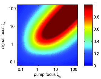
Figure 7: (color online) Dependence of the signal collection probability on the focus of the pump and signal modes for near-degenerate SPDC ($k_{\text{s}}\approx k_{\text{i}}\approx k_{\text{p}}/2$).

If one takes $\xi_{\text{s}}=\xi_{\text{i}}=\xi_{\text{p}},$ which locally maximizes both $P_{\text{si}}$ and $P_{\text{s}},$ the signal heralding ratio reduces to the simple expression

$$\eta_{\text{s}}=\frac{k_{\text{i}}}{k_{\text{p}}}\left(\frac{k_{\text{s}}}{k_{\text{p}}}+1\right).$$ (55)

An analogous expression exists for $\eta_{\text{i}}$. These expressions give $\eta_{\text{s}}=\eta_{\text{i}}=0.75$ for near-degenerate SPDC (for which $k_{\text{s}}\approx k_{\text{i}}\approx k_{\text{p}}/2$) and values less than 0.75 for the non-degenerate case. However, higher heralding ratios are possible with different focusing conditions. The optimal source configuration with regard to both heralding and brightness is not a single set of parameter values, but a curve in parameter space having the property that $\eta_{\text{s}}$ (or $\eta_{\text{si}},$ if that is of interest) cannot be increased without decreasing $P_{\text{si}},$ and vice versa. Numerical methods were used to find the values $(\xi_{\text{s}},\xi_{\text{i}},\xi_{\text{p}})$ that maximize either $\eta_{\text{s}}$ or $\eta_{\text{si}}$ at 50 values of $P_{\text{si}}$ covering the range from 0 to $\max P_{\text{si}}$. The resulting points are plotted versus $\xi_{\text{p}}$ in Fig. 8 for the case $k_{\text{s}}\approx k_{\text{i}}\approx k_{\text{p}}/2$. Fig. 8 shows that it is possible to achieve very high heralding ratios, but only with a substantial reduction in brightness: a factor of at least 4 to achieve $\eta_{\text{s}}\geq 0.95$ and a factor of at least 10 to achieve $\eta_{\text{si}}\geq 0.95$. That is, there is a trade-off between brightness and heralding ratio, which is somehwat worse for symmetric heralding than asymmetric heralding. Both $\eta_{\text{s}}$ and $\eta_{\text{si}}$ approach unity in the limit that the pump is collimated ($\xi_{\text{p}}\rightarrow 0$). In this limit the best trade-off between $P_{\text{si}}$ and $\eta_{\text{si}}$ is achieved with $\xi_{\text{s}}=\xi_{\text{i}}\gg\xi_{\text{p}},$ while the best trade-off between $P_{\text{si}}$ and $\eta_{\text{s}}$ is achieved with $\xi_{\text{i}}\approx 3\xi_{\text{s}}\approx 3\xi_{\text{p}}$. The trade-offs between $P_{\text{si}}$ and $\eta_{\text{s}}$ or $\eta_{\text{si}}$ are found to be slightly worse in the non-degenerate case than the near-degenerate case.

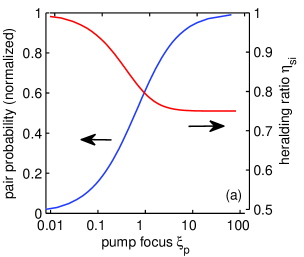
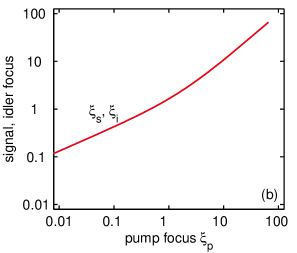
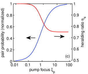
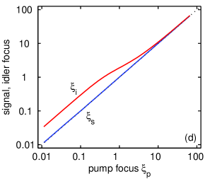
Figure 8: (color online) (a,b) Simultaneous optimization of the total collection probability $P_{\text{si}}$ and the symmetric heralding ratio $\eta_{\text{si}}$. (c,d) Simultaneous optimization of $P_{\text{si}}$ and the signal heralding ratio $\eta_{\text{s}}$. Panels (b) and (d) plot the focal parameters that yield the optimal curves shown in (a) and (c), respectively. In (a) and (c) the collection probability goes with the left axis and the heralding ratio goes with the right axis.

VIII Discussion

Perhaps the most significant finding of this study is that there exist focusing conditions ($\xi_{\text{p}},\xi_{\text{s}},\xi_{\text{i}}\sim 2.5$) that simultaneously bring the brightness, heralding ratio, and spectral purity to substantial fractions of their maximal values. Whenever $n_{\text{p}}^{\prime}$ lies between $n_{\text{s}}^{\prime}$ and $n_{\text{i}}^{\prime},$ a spectral purity of at least 0.94 can be obtained with at least 74% of the maximum achievable brightness, while the heralding ratio is at least 0.75 (for near-degenerate SPDC). Maximum brightness can be achieved with tighter focusing at the cost of reducing the spectral purity (to 0.7 at worst) The worst trade-off is between brightness and heralding ratio: focusing conditions that yield a symmetric (asymmetric) heralding ratio of 0.95 or better reduce the brightness to 10% (25%) of its maximal value; however the spectral purity remains 0.84 or better.

Another notable finding of this study, which to my knowledge has not been reported previously, is that many important properties of the collected SPDC state are essentially scale invariant. To the extent that the parameter $C$ (see (14)) is negligibly small, the joint collection probability, heralding ratios, and spectral purity are determined by the dimensionless ratios $L/k_{j}w_{j}^{2}$ and $\Delta\omega_{\text{p}}L/c$. Changing the crystal length has no effect on these three quantities if the pump duration and confocal ranges are also scaled by the same factor. In the end, the crystal length merely sets the bandwidth of the system, with longer crystals yielding (or requiring) smaller bandwidths. The idea that a longer crystal does not yield a brighter source is perhaps surprising, since longer crystals yield higher SPDC efficiencies when the pump is collimated or weakly focused. Why this is not so for optimally focused sources may be understood by noting that, although a shorter crystal has a shorter interaction length (which decreases the spatial mode overlap), it also allows the modes to be focused more tightly (which increases the mode overlap). Of course, this argument does not hold for arbitrarily short crystals; at some point, the focusing becomes so strong and the bandwidths become so large that the paraxial approximation implicit in (7), as well as approximations such as (20), break down. At the other extreme, very long crystals may also show worse than expected performance due to the challenge of manufacturing very long crystals of high quality.

Some of the results obtained here appear to agree with prior works, while others appear to differ from prior works. The focusing condition $\xi_{\text{s}}=\xi_{\text{i}}=\xi_{\text{p}}=2.84$ which maximizes the joint spectral density of SPDC is the same as that found by Boyd and Kleinman for maximizing second harmonic generation Boyd1968 . This makes sense, since SHG with a monochromatic Gaussian input beam produces a monochromatic Gaussian second harmonic field; optimization of SHG then amounts to finding the parameters of the Gaussian modes that maximize the spatial overlap, which is precisely what was done in section III. More recently, Ljunggren and Tengner Ljunggren2005 have performed numerical studies yielding the optimizing conditions $2\xi_{\text{p}}=1.7,$ $2\xi_{\text{s}}=2\xi_{\text{i}}=2.3$, and the prediction that the optimized joint probability goes as $\sqrt{L}$ (rather than being independent of $L$ as claimed here). These discrepencies may be due to two key differences in approach: In Ljunggren2005 , optimal focusing conditions are obtained for $\Phi=0$, whereas here and in Boyd1968 the condition $\Phi=-1.04\pi$ is found to yield a slightly higher spectral density. Additionally, Ljunggren2005 employs a plane-wave approach in which the diffraction of the pump mode is effectively ignored; this approximation is also made in Castelletto2005 , Dragan2004 and Ling2008 . In the present study the pump is treated as a diffracting paraxial beam. Experiments to date are insufficient to resolve these differences as they cover a limited range of crystal lengths and focal parameters, and are complicated by poor repeatability (changing the focus of a beam, or replacing a crystal with one of different length, generally necessitates realignment).

The results of this study are intended to be useful for designing and predicting the approximate performance of a promising class of SPDC sources. A number of points should be kept in mind, however. Firstly, all the results presented here apply to the collected part of the biphoton state; many features of the emitted SPDC light are lost or substantially altered when the state is projected onto the Gaussian collection modes. Secondly, while care was taken to confirm the general viability of the approximations employed, it is not difficult to envision sources that would violate the assumptions of this analysis and exhibit quantitatively or qualitatively different performance. In particular, results obtained here may not be reliable for very short sources ($L\lesssim\operatorname{mm}$), sources with very short poling periods ($\Lambda\lesssim 5\operatorname{\mu m}$), and/or sources employing quasi-phasematching of order $m>1$. Thirdly, certain physical details deemed inconsequential—such as the vector diffraction of the Gaussian beams, the optical anisotropy of nonlinear crystals, and the proper normalization of electromagnetic modes quantized in a dielectric—were simply ignored. Fourthly, a limitiation of this study is that it does not apply to angle-tuned sources in which beam walk-off plays a role. However, since walk-off decreases spatial overlap, it is not clear that such sources could achieve better overall performance than the co-linear sources considered here. Finally, of all the results obtained here, only those in section III are potentially applicable to frequency-degenerate type I sources. The quadratic relationship between frequency and phase mismatch in these sources substantially complicates analysis; however, the possibility that these sources might have different scaling laws makes them potentially worth a comparable study.

IX Summary

In summary, I have presented here a new theoretical study of SPDC addressing multiple properties of the emitted photons that are important in various applications. Analysis was restricted to the promising class of SPDC sources involving focused, co-linear Gaussian modes for the pump field and collected photons. Analytical and numerical calculations yielded approximate predictions for the peak spectral density, photon bandwidths, absolute pair collection probability, heralding ratio, and spectral purity. A scaling law was found which shows most of these properties to be ultimately independent of crystal length. It was also found that such sources can simultaneously exhibit high brightness (predicted $10^{-9}$ pairs/pump photon), high spectral purity ($\geq 0.94$), and moderately high heralding ratio ($\gtrsim 0.75$) when the confocal ranges of the modes are on the order of half the crystal length. Higher heralding ratios can be achieved, at the cost of significantly reduced brightness, by focusing the modes less tightly. The results of this study are applicable to “typical” SPDC sources, excluding sources of very short length, very short poling period, or very large bandwidth. Frequency-degenerate type I sources, which often do not satisfy these criteria, may be amenable to a similar kind of study.

This work was sponsored by the Intelligence Advanced Research Projects Activity (IARPA) and by the Laboratory Directed Research and Development Program of Oak Ridge National Laboratory, managed by UT-Battelle, LLC, for the U. S. Department of Energy.

The author thanks W. P. Grice, T. S. Humble, and P. G. Evans for helpful discussions.

References

- (1) A. Politi, J. C. F. Matthews, M. G. Thompson, and J. L. O’Brien. IEEE Journal on Selected Topics in Quantum Electronics 15, 1673 (2009).
- (2) M. Peev et al. New Journal of Physics 11, 075001 (2009).
- (3) F. Wong, J. Shapiro, and T. Kim. Laser Physics 16, 1517 (2006).
- (4) A. Fedrizzi, T. Herbst, A. Poppe, T. Jennewein, and A. Zeilinger. Optics Express 15, 598 (2007).
- (5) W. P. Grice, A. B. U’Ren, and I. A. Walmsley. Phys. Rev. A 64, 063815 (2001).
- (6) A. U’Ren, Y. Jeronimo-Moreno, and H. Garcia-Gracia. Physical Review A 75, 23810 (2007).
- (7) P. J. Mosley, J. S. Lundeen, B. J. Smith, and I. A. Walmsley. Journal of Modern Optics 56, 179 (2009).
- (8) T. Humble and W. Grice. Physical Review A 75, 022307 (2007).
- (9) C. Kurtsiefer, M. Oberparleiter, and H. Weinfurter. Phys. Rev. A 64, 023802 (2001).
- (10) F. Bovino, P. Varisco, A. Colla, G. Castagnoli, G. Di Giuseppe, and A. Sergienko. Opt. Comm. 227, 343 (2003).
- (11) A. Dragan. Phys. Rev. A 70, 053814 (2004).
- (12) R. Andrews, E. Pike, and S. Sarkar. Opt. Expr. 12, 3264 (2004).
- (13) S. Castelletto, I. Degiovanni, G. Furno, V. Schettini, A. Migdall, and M. Ware. IEEE Trans. Instrum. Meas. 54, 890 (2005).
- (14) D. Ljunggren and M. Tengner. Phys. Rev. A 72, 062301 (2005).
- (15) A. Ling, A. Lamas-Linares, and C. Kurtsiefer. Physical Review A 77, 043834 (2008).
- (16) P. Kolenderski, W. Wasilewski, and K. Banaszek. Physical Review A 80, 013811 (2009).
- (17) C. Hong and L. Mandel. Physical Review A 31, 2409 (1985).
- (18) P. Evans, J. Schaake, R. Bennink, T. Humble, and W. Grice (unpublished).
- (19) G. D. Boyd and D. A. Kleinman. Journal of Applied Physics 39, 3597 (1968).
- (20) S. Carrasco, A. V. Sergienko, B. E. Saleh, M. C. Teich, J. P. Torres, and L. Torner. Phys. Rev. A 73 063802 (2006).
- (21) P. G. Kwiat, K. Mattle, H. Weinfurter, A. Zeilinger, A. V. Sergienko, and Y. H. Shih. Phys. Rev. Lett. 75, 4337 (1995).
- (22) Z. Zhao, K. A. Meyer, W. B. Whitten, R. W. Shaw, R. S. Bennink, and W. P. Grice. Phys. Rev. A 77, 063828 (2008).
- (23) C.-Y. Lu, X.-Q. Zhou, O. Guhne, W.-B. Gao, J. Zhang, Z.-S. Yuan, A. Goebel, T. Yang, and J.-W. Pan. Nat Phys 3, 91 (2007).
- (24) M. Radmark, M. Zukowski, and M. Bourennane. Physical Review Letters 103, 150501 (2009).
- (25) W. Wieczorek, R. Krischek, N. Kiesel, P. Michelberger, G. Toth, and H. Weinfurter. Physical Review Letters 103, 020504 (2009).
- (26) R. Prevedel, G. Cronenberg, M. Tame, M. Paternostro, P. Walther, M. Kim, and A. Zeilinger. Physical Review Letters 103, 020503 (2009).
- (27) A. U’Ren, E. Mukamel, K. Banaszek, and I. Walmsley. Phil. Trans. Roy. Soc. Lond. A 361, 1493 (2003).
- (28) T. Humble and W. Grice. Physical Review A 77, 022312 (2008).
- (29) C. K. Law, I. A. Walmsley, and J. H. Eberly. Phys. Rev. Lett. 84, 5304 (2000).